A Hierarchical Method for Transient Stability Prediction of Power Systems Using the Confidence of a SVM-Based Ensemble Classifier

Abstract

Machine learning techniques have been widely used in transient stability prediction of power systems. When using the post-fault dynamic responses, it is difficult to draw a definite conclusion about how long the duration of response data used should be in order to balance the accuracy and speed. Besides, previous studies have the problem of lacking consideration for the confidence level. To solve these problems, a hierarchical method for transient stability prediction based on the confidence of ensemble classifier using multiple support vector machines (SVMs) is proposed. Firstly, multiple datasets are generated by bootstrap sampling, then features are randomly picked up to compress the datasets. Secondly, the confidence indices are defined and multiple SVMs are built based on these generated datasets. By synthesizing the probabilistic outputs of multiple SVMs, the prediction results and confidence of the ensemble classifier will be obtained. Finally, different ensemble classifiers with different response times are built to construct different layers of the proposed hierarchical scheme. The simulation results show that the proposed hierarchical method can balance the accuracy and rapidity of the transient stability prediction. Moreover, the hierarchical method can reduce the misjudgments of unstable instances and cooperate with the time domain simulation to insure the security and stability of power systems.

1. Introduction

With the continuous growth of electricity demand and the enlargement of the power system interconnection scale, power systems are becoming increasingly complex and have been forced to operate closer to their stability limits. Hence, ensuring the security of power systems has become more challenging. Transient instability has historically been the dominant stability problem in power systems [1]. Therefore, the study on the transient stability has great significance for the secure and stable operation of power systems.

Transient, or large-disturbance rotor angle stability, refers to the ability of an interconnected power system to maintain synchronism after a severe disturbance [1], and the relevant literature is rich. Time domain simulation is the most traditional transient stability analysis method. However this method depends on exact models and parameters, and it is time-consuming which makes it hard to apply online. Other traditional methods, such as the transient energy function method and extended equal-area criterion, have model limitations which makes it hard for them to give efficient and precise results for large-scale power systems. Recently, the machine learning techniques, with high computing speed and precision, as well as the capacity of mining the potential useful information from among massive sets of data, have been used to predict the transient stability [2,3,4,5,6,7,8,9,10,11,12,13,14,15,16,17,18,19]. The transient stability prediction can be treated as a two-class classification (stable and unstable) problem and solved by machine learning methods. A set of appropriate features/attributes is selected to generate the offline training sets, then an appropriate classification method is utilized to predict the transient stability status.

There are two kinds of machine learning-based methods with different types of inputs [2]. One uses pre-fault steady-state variables as the original data, the machine learning method will be used to build the mapping between the steady-stable variables and the transient stability status with respect to an anticipated but not yet occurred contingency [2,3,4,5]. Once the current status is identified as insecure, preventive control can be carried out to modify the system to a secure state. However, when a serious fault happens, or failure of primary relay protection, the power system may still be unstable even if the preventive control has been conducted. Therefore we should emphasize importance of the study on transient stability prediction using post-fault responses. Because the post-fault responses carry information about the influence of the faults on the power system, the prediction is independent of the faults. This arises the second way of transient stability prediction based on machine learning techniques.

With the development of wide-area measurement systems, the dynamic response of power systems after a disturbance can be measured by phasor measurement units, which provides data support for post-fault transient stability prediction. However, it brings forward strict requirements regarding the prediction accuracy and speed because a fault has already occurred. Recently, the construction of input data and the improvement of machine learning methods to increase the accuracy have been the main research focus. Methods such as neural networks [6,7,8], decision trees (DTs) [9,10,11], support vector machines (SVMs) [12,13,14,15], fuzzy theory [16,17] and some ensemble classifiers [18,19] had been used for post-fault transient stability analysis.

In fact, a classifier should possess high prediction accuracy, but it is also important to estimate the credibility of each classification result, or the confidence level. The existing transient stability prediction only provides a prediction result but seldom considers the confidence level. When two stable results are provided by a classifier, one with lower confidence whereas the other with higher confidence, these two situations should be treated differently. In [14], the results are divided into credible and incredible simply based on the SVM results, but lack further research on the definition and application of confidence indices.

The post-fault dynamic responses vary with time, and the selection of the duration time of the response data, called response time in this paper, is always a problem that needs to be solved for post-fault transient stability prediction. The sooner the prediction is completed, the longer the time available to take actions to avoid a possible collapse is [13]. Thus, selecting too long a response time cannot meet the requirements of online application. However, the responses with little duration time may still not display distinguishing characteristics, which increases the difficulty to achieve high accurate prediction, so the accuracy and speed are contradictory. In the literature, a relative optimal response time will be determined by the comparison between the accuracy and time of different classifiers with different response times. The selections of response times are different, e.g., 50 ms in [12], 150 ms and 300 ms in [17], 200 ms in [11]. Therefore it is hard to draw definite conclusions about that how long the best response time for any power system is.

Among the various machine learning methods, SVM has demonstrated better performance in transient stability prediction. The SVM classifier can not only provide the prediction results, but also give out the “distance” between the instance and stable boundary [14], which can be further used to define the confidence index. Based on the aforementioned analysis, we propose in this paper a SVM-based ensemble classifier and its confidence evaluation index. Most importantly, the proposed confidence index provides the credibility evaluation of transient stability prediction results and a new solution for the selection of response time, helping to construct a comprehensive hierarchical method which can balance the accuracy and rapidity.

The rest of this paper is organized as follows: Section 2 introduces the generation of datasets for transient stability prediction. Section 3 introduces the SVM-based ensemble classifier and its confidence index. Based on the contents in Section 2 and Section 3, the proposed hierarchical method will be introduced in Section 4. Results and Discussions of comprehensive case studies on 16-machine 68-bus power system are conducted in Section 5. The conclusions are given in Section 6.

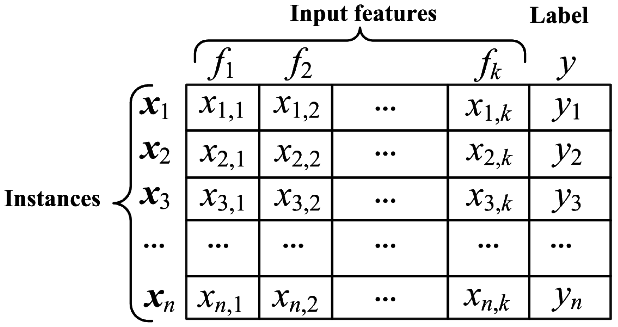
2. Generation of Dataset

In terms of machine learning-based method for transient stability prediction, the first step is to generate the original dataset, shown in Figure 1.

Generally, the transient stability dataset is generated by the time domain simulations [19]. When a power system is determined, the uncertainties associated with load levels, network configurations, fault types, locations and clearing times need to be modeled, then the time domain simulations will be carried out to determine whether the system is transient stable or not. In Figure 1, y_i ∈ {+1,−1} is the transient stability label, y_i = +1 and y_i = −1 represent the stable and unstable respectively. Finally, n instances in total with their transient stability labels are obtained.

Massive amounts of data will be generated during the time domain simulation, e.g., the generator electromagnetic powers, rotor angles and speeds, bus voltages and transmission line powers. Using all the variables will make the scale of the dataset too large, and even cause a “dimension disaster” problem. Thus it is necessary to extract some important features to describe the instances.

Transient stability, or large-disturbance rotor angle stability, refers to the ability of all the generators to maintain synchronism after a severe disturbance. Therefore the generator dynamic responses carry important information for transient stability prediction. Varieties of input features have been utilized in previous research. From the perspective of whether the number of features is related to the scale of the power system, the input features can be divided into the component features and system features. The component features are the variables of individual components, e.g., the rotor angles, electromagnetic powers of generators, etc. The system features are the combined variables that are computed by the variables of multiple components. The most major characteristic of the system features is that the feature number is independent of the power system scale.

On the basis of the related literature and our comprehension of transient stability, we utilized the statistics of the generator variables to construct the input features, shown in

Table 1. Construction of the input features.

Feature	Description	Feature	Description
f1	Average{Pmi(tb)}	f18	Max{ῶi(tk)} + Min{ῶi(tk)}
f2	Average{Pei(tFOT)/Pmi(tFOT)}	f19	Coefficient of variation{ῶi(tk)}
f3	Max{Pei(tFOT)/Pmi(tFOT)}	f20	αCOI(tk)
f4	Min{Pei(tFOT)/Pmi(tFOT)}	f21	Average{|ᾶi(tk)|}
f5	Average{Pei(tk)/Pmi(tk)}	f22	Variance{ᾶi(tk)}
f6	Max{Pei(tk)/Pmi(tk)}	f23	Max{ᾶi(tk)} − Min{ᾶi(tk)}
f7	Min{Pei(tk)/Pmi(tk)}	f24	Max{ᾶi(tk)} + Min{ᾶi(tk)}
f8	δCOI(tk)	f25	Coefficient of variation{ᾶi(tk)}
f9	Average{|${\tilde{\mathsf{\delta }}}_i$(tk)|}	f26	Average{EKi(tk)}
f10	Variance{${\tilde{\mathsf{\delta }}}_i$(tk)}	f27	Variance(EKi(tk))
f11	Max{${\tilde{\mathsf{\delta }}}_i$(tk)} − Min{${\tilde{\mathsf{\delta }}}_i$(tk)}	f28	Max{EKi(tk)} − Min{EKi(tk)}
f12	Max{${\tilde{\mathsf{\delta }}}_i$(tk)} + Min{${\tilde{\mathsf{\delta }}}_i$(tk)}	f29	Max{EKi(tk)} + Min{EKi(tk)}
f13	Coefficient of variation{${\tilde{\mathsf{\delta }}}_i$(tk)}	f30	Coefficient of variation{EKi(tk)}
f14	ωCOI(tk)	f31	Max{dEKi/dt} − Min{dEKi/dt}|t = tk
f15	Average{|ῶi(tk)|}	f32	v(tk)
f16	Variance{ῶi(tk)}	f33	δGL(tk) − δGB(tk)
f17	Max{ῶi(tk)} − Min{ῶi(tk)}	f34	ωGL(tk) − ωGB(tk)

. The statistical features can be viewed as the system features and their amount is independent of the power system scale. All the input features are defined in the following subsections.

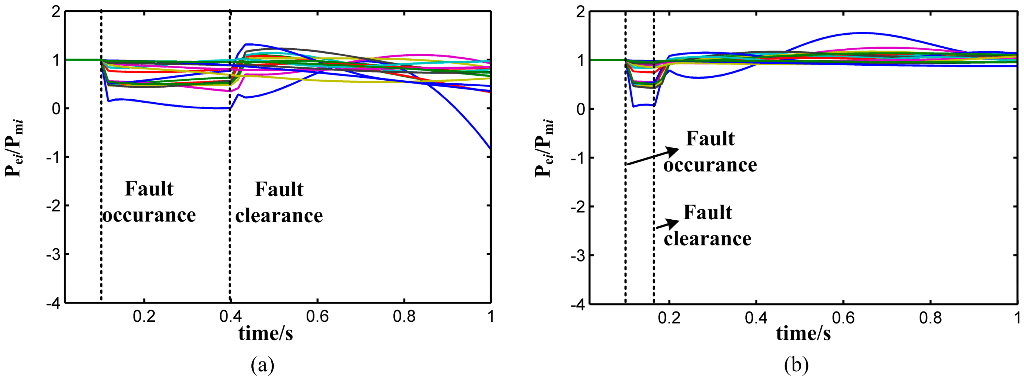
2.1. Generator Electromagnetic Powers

Generator electromagnetic powers have been utilized to construct the input features [14]. The power system is in equilibrium before a fault occurs, and the average of all the generator electromagnetic powers reflects the load level of the current status. When a fault occurs, the electromagnetic power will suddenly change but the mechanical power cannot because of the inertia of the governor. Thus the ratio of the electromagnetic and mechanical power of the i-th generator, P_ei/P_mi, reflects the relative variation of the i-th generator electromagnetic power following this fault. Figure 2 shows the variation of the P_ei/P_mi of a 16-machine 68-bus system (see Section 5) for the unstable and stable cases. The electromagnetic power is equal to the mechanical power of each generator before a fault occurs, that is P_ei/P_mi = 1. When the fault occurs, the value of P_ei/P_m will reduce and remain at a low level until the fault is cleared. After the fault clearance, the value of P_ei/P_mi reflects the recovery of the generator electromagnetic power. The value of P_ei/P_mi will tend to 1 for the stable case. On the contrary, when the system is stable, the value of P_ei/P_mi of one generator is far away from 1. Therefore the value of P_ei/P_mi can be used to identify the transient stability status. Based on the statistics of generator electromagnetic powers, totally seven input features, f₁–f₇ shown in Table 1 are defined as the input features, where t_b is the time before the fault occurs, t_FOT is the fault occurrence time.

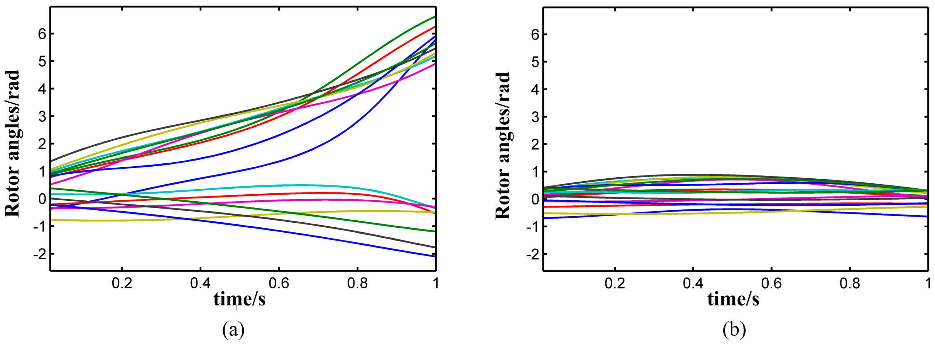
2.2. Generator Rotor Angles

Transient stability is dependent on the dynamics of generator rotor angles, which have been used as the input feature in many literatures [8,9,14,19]. The concept of reference centre angle is widely used in transient stability assessments, and called the centre of inertia (COI) [20]. For an N-generator power system, the COI reference of the rotor angle at t = t_k after the fault clearance, δ_COI(t_k), is:

$${\mathsf{\delta }}_{\mathrm{COI}}(t_k)={\displaystyle \sum _{i=1}^N{M}_i{\mathsf{\delta }}_i\left(t_k\right)}/{\displaystyle \sum _{i=1}^N{M}_i}$$

(1)

where δ_i(t_k) and M_i are the rotor angle and inertia coefficient of the i-th generator at at t = t_k after the fault clearance. Besides, the COI reference of rotor speed and acceleration, ω_COI(t_k) and α_COI(t_k), are shown in Equations (2) and (3) respectively:

$${\mathsf{\omega }}_{\mathrm{COI}}(t_k)=\frac{d{\mathsf{\delta }}_{\mathrm{COI}}}{dt}|t=t_k$$

(2)

$${\mathsf{\alpha }}_{\mathrm{COI}}(t_k)=\frac{d{\mathsf{\omega }}_{\mathrm{COI}}}{dt}|t=t_k$$

(3)

In Equations (2) and (3), the derivative can be calculated using a difference approximation. From here on, the relative rotor angle, speed and acceleration of the i-th generator in the COI frame at t = t_k after the fault clearance are ${\tilde{\mathsf{\delta }}}_i\left(t_k\right)$ = δ_i(t_k) − δ_COI(t_k), ῶ_i(t_k) = ω_i(t_k) − ω_COI(t_k) and ᾶ_i(t_k) = α_i(t_k) − α_COI(t_k) respectively.

The kinetic energy of the i-th generator, EK_i(t_k), can also be used for transient stability prediction. It is defined as follows:

$$E{K}_i(t_k)=\frac{1}{2}{M}_i{({\mathsf{ῶ}}_i(t_k))}^2$$

(4)

Figure 3, Figure 4, Figure 5 and Figure 6 show the variations of all the generator rotor angles, speeds, accelerations and kinetic energy of the 16-machine 68-bus system after the fault clearance. When the system is stable, the values of the rotor angles, speeds, accelerations and kinetic energy are low. However, the values of these quantities change drastically. This inspires us to extract the statistical features, such as maximum, minimum, variance etc. of the post-disturbance trajectories to construct the input features. Therefore, based on the statistics of the aforementioned rotor angles, speeds, accelerations, kinetic energy, 24 input features, f₈–f₃₁ shown in Table 1, are utilized for transient stability prediction.

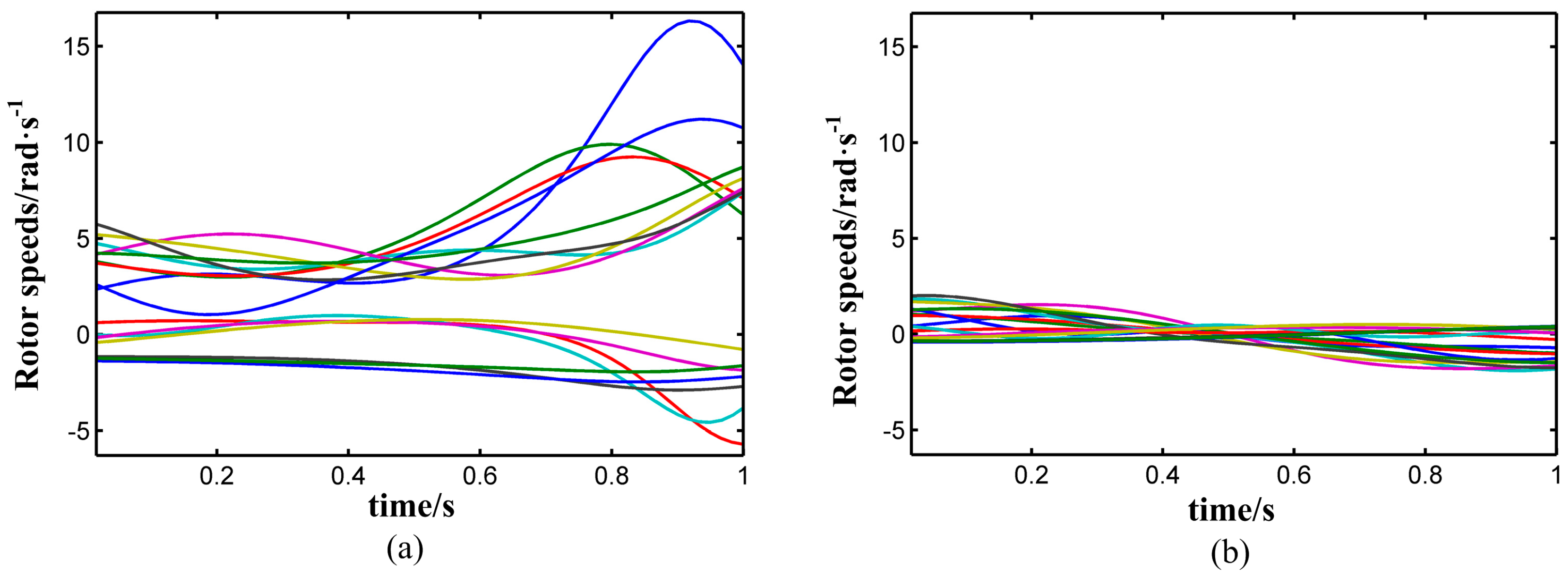
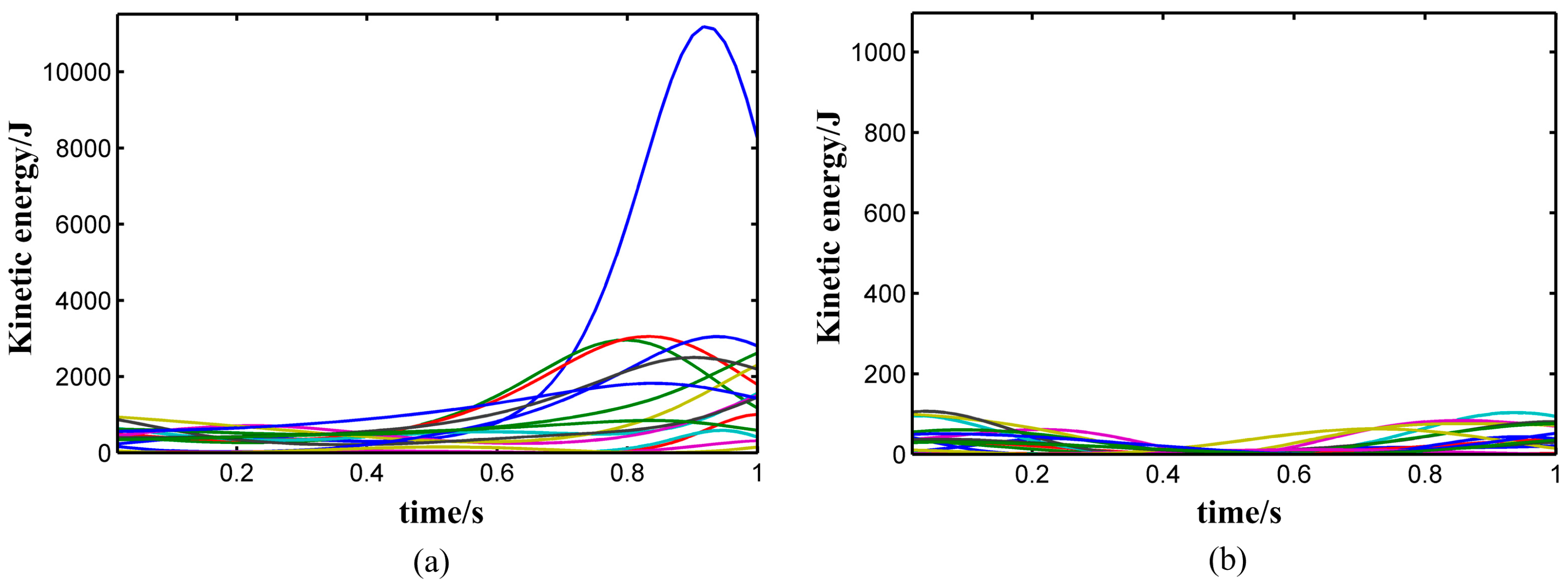
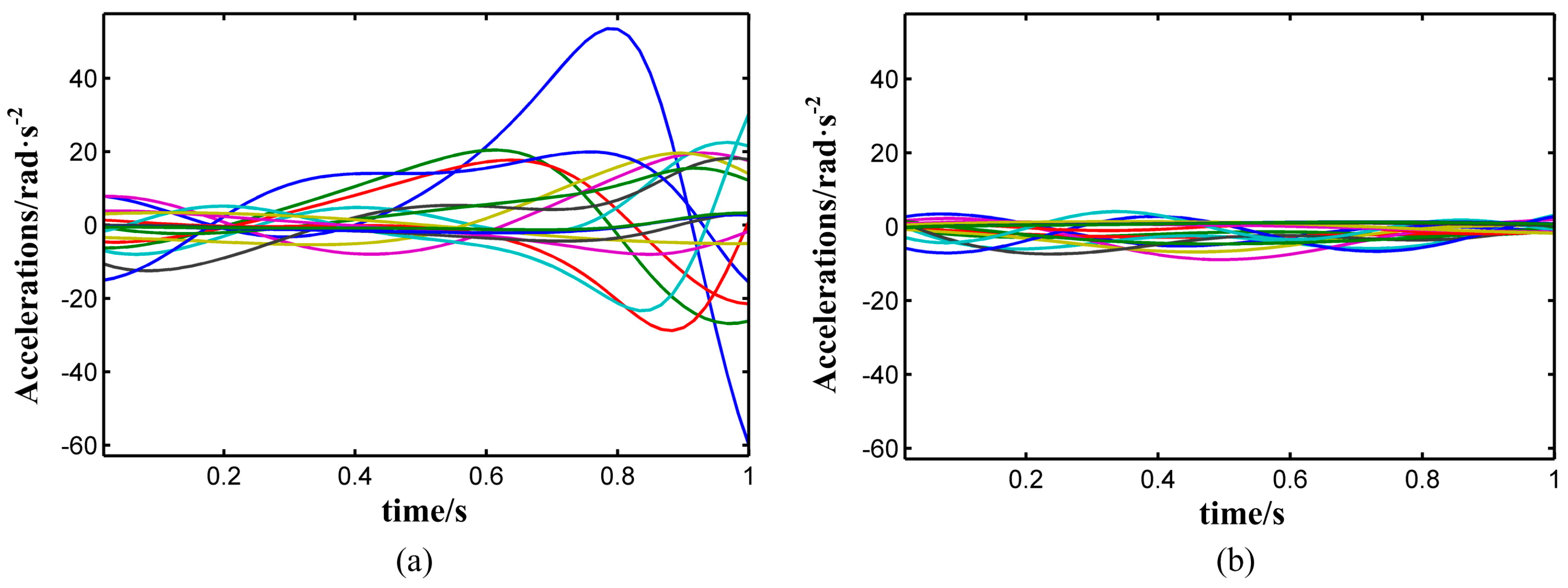
2.3. Other Useful Features

Another useful quantity for transient stability prediction is the dot product of the rotor angles and speed [17], v(t_k):

$$v(t_k)={\displaystyle \sum _{i=1}^N({\mathsf{ῶ}}_i(t_k)\times ({\tilde{\mathsf{\delta }}}_i(t_k)-{\tilde{\mathsf{\delta }}}_i(0+)))}$$

(5)

Where ${\tilde{\mathsf{\delta }}}_i$(0+) and ${\tilde{\mathsf{\delta }}}_i$(t_k) are the relative rotor angle of the i-th generator in the COI frame at the fault clearing instant and t_k after the fault clearance, respectively, ῶ_i(t_k) is the relative rotor speed of the i-th generator at t = t_k after the fault clearance.

The generators with the biggest and smallest rotor acceleration may be the key generators leading to the separation of rotor angles. In this research, these two generators are labelled as GL and GB, respectively. Then rotor angle difference and speed difference of these two generators are also used as the input features.

Finally, the features shown in Table 1 form the 34 input features for transient stability prediction. These 34 features are the descriptions of all the generated instances shown in Figure 1. The dataset can be expressed as (x_i, y_i), where i = 1,…, n, x_i = [x_ij]_1×34. To unify the original data from different variables with different dimensions and accelerate the conversion speed, the original data are usually normalized using Equation (6):

$${x^{*}}_{ij}=\frac{x_{ij}-\underset{i}{\min }(x_{ij})}{\underset{i}{\max }(x_{ij})-\underset{i}{\min }(x_{ij})}$$

(6)

After the normalization, the original data are mapped into the range of [0, 1] and will be processed by the following machine learning methods in Section 3. For simplicity, the normalized data are also marked as x_i = [x_ij]_1×34 in this paper.

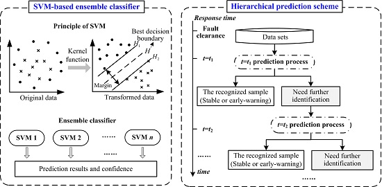
3. Support Vector Machine-Based Ensemble Classifier and Its Confidence Evaluation

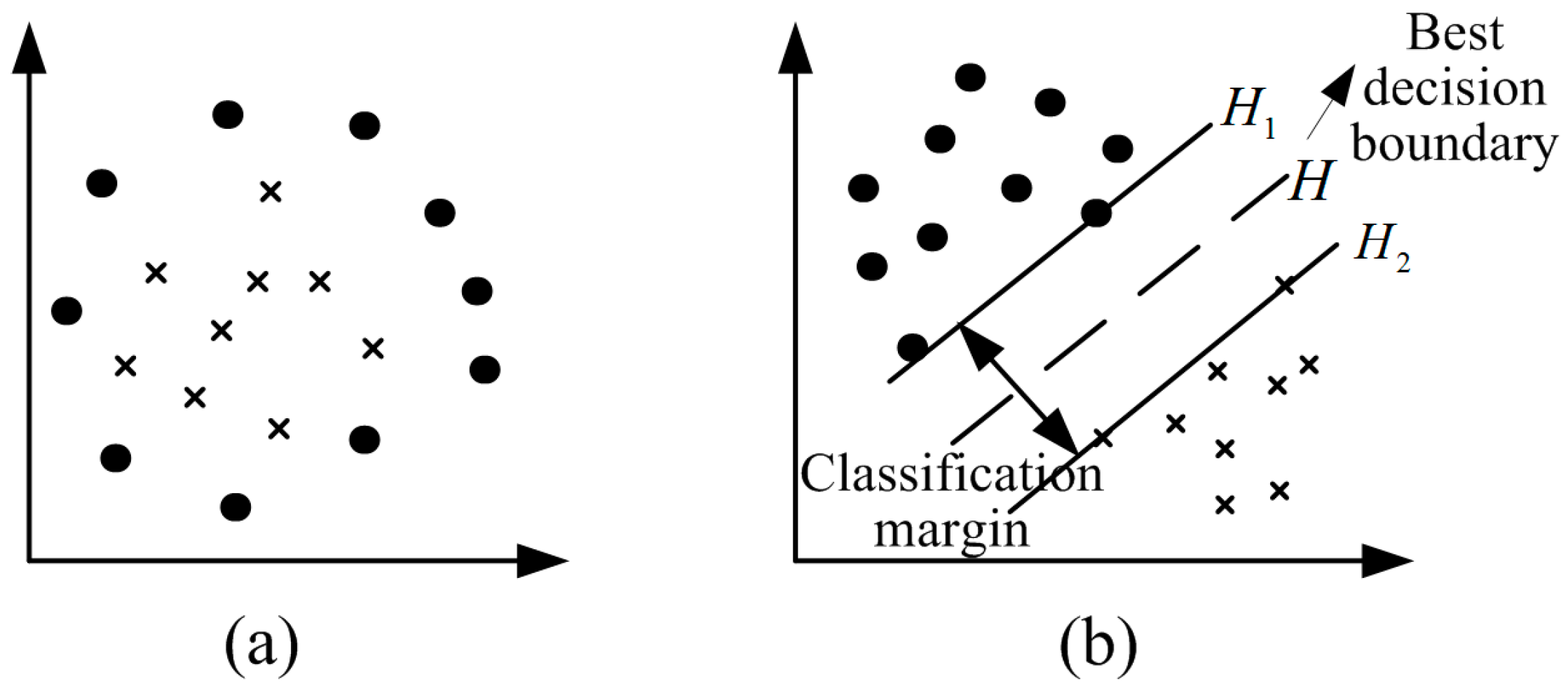
3.1. Principle of Support Vector Machine

After the dataset (x_i, y_i), or a set of instance-label pairs, is obtained, a machine learning method should be selected and utilized to build the mapping between the input features and transient stability status y = f(x). SVM algorithm, which is based on the statistical learning and follows the principle of the structural risk minimization [21], has been widely used for transient stability prediction [12,13,14,15]. In this research, SVM will be studied and used to build the transient stability classifier.

Figure 7 shows the basic principle of SVM. The actual dataset is usually linearly inseparable (Figure 7a), then this dataset is transformed into a new space using a nonlinear mapping, also called as the kernel function K(x_i,x_j). The transformed data may become linearly separable that much easier to find the best decision boundary with the maximum classification margin, also the minimum classification risk (Figure 7b).

The best decision function y = f(x) can be expressed as:

$$f(x)=\mathrm{sgn}\{{\displaystyle \sum _{i=1}^{N^{\mathrm{sv}}}{\mathsf{\alpha }}_i{y}_i^{\mathrm{sv}}K(x_i^{\mathrm{sv}},x)+b}\}$$

(7)

where sgn{} is sign function, N^sv is the number of support vectors, x_i^sv is the i-th support vectors and y_i^sv is the corresponding label, b ∈ R, and α_i is the Lagrange multiplier obtained from solving the following optimization problem:

$$\begin{array}{cc}\min & \frac{1}{2}{\displaystyle \sum _{i=1}^{N^{\mathrm{sv}}}{\displaystyle \sum _{j=1}^{N^{\mathrm{sv}}}{\mathsf{\alpha }}_i{\mathsf{\alpha }}_j{y}_i^{\mathrm{sv}}{y}_j^{\mathrm{sv}}K(x_i^{\mathrm{sv}},x)}}-{\displaystyle \sum _{i=1}^{N^{\mathrm{sv}}}{\mathsf{\alpha }}_i}\\ s.t.& C\ge {\mathsf{\alpha }}_i\ge 0,i=1,...,l\\ & {\displaystyle \sum _{i=1}^{N^{\mathrm{sv}}}{\mathsf{\alpha }}_i{y}_i^{\mathrm{sv}}}=0\end{array}$$

(8)

where C ∈ R is the penalty parameter.

Common kernel functions include the polynomial, Gaussian radial basis function (RBF), and sigmoid function. In [22], it is verified that the RBF can approximate to any functions with arbitrary small error. In addition, many related articles had utilized the SVM with RBF for transient stability prediction [12,13,14,15]. Therefore the kernel function in this research is the RBF:

$$K(x_i^{\mathrm{sv}},x)=\exp \left\{-\frac{{\left|x-x_i^{\mathrm{sv}}\right|}^2}{{\mathsf{\sigma }}^2}\right\}$$

(9)

where σ ∈ R is the width of the Gaussian.

Two parameters, C and σ, need to be determined before the generation of the final SVM classifier. Generally, the optimal parameters should be found through a grid-search process [12,13,14,15].

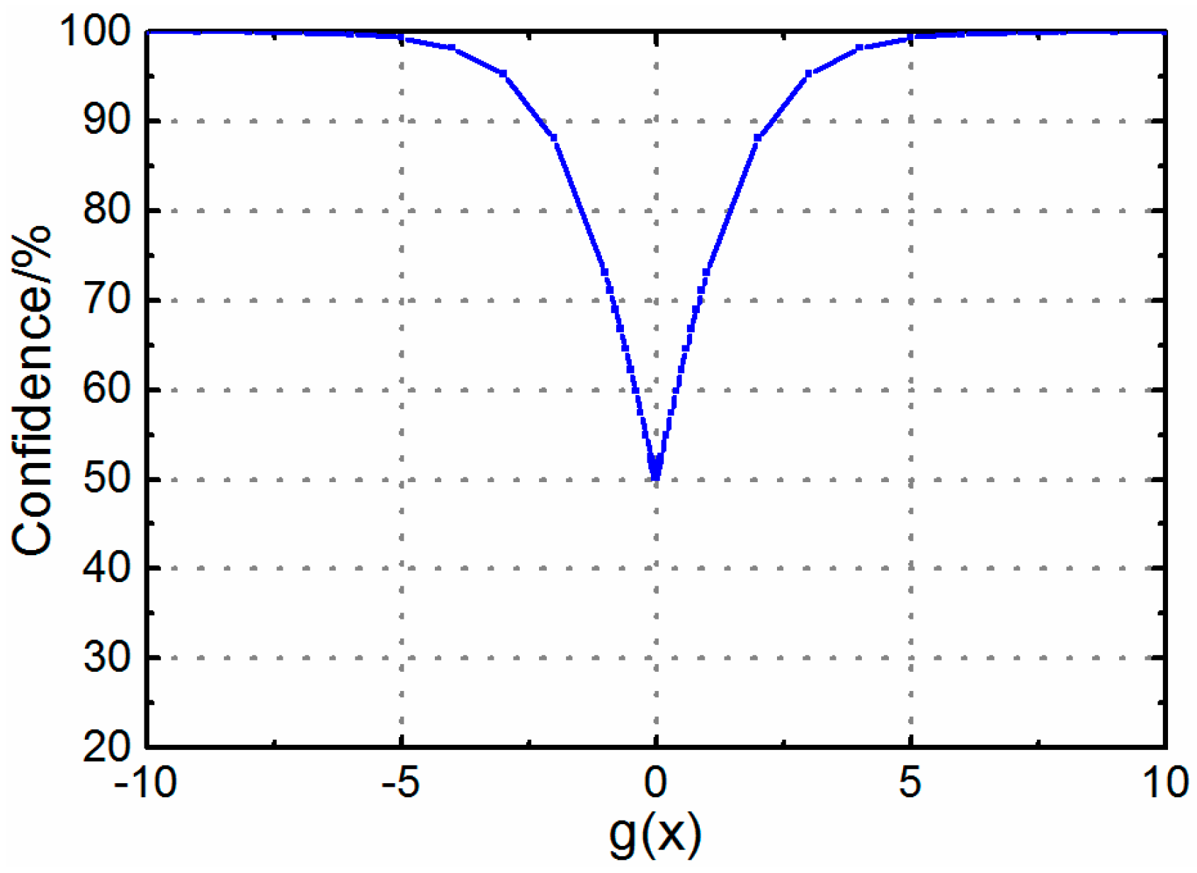
3.2. Confidence Evaluation of Support Vector Machine

The nature of the aforementioned SVM decision function of Equation (7) is a sign function. That means we can only know the instance is stable or unstable from the output of SVM, but not the distance between the instance and the optimal decision boundary. One method to improve the SVM output to a probabilistic output form is [23]:

P(C₊₁|x) = 1/(1 + e^−g(x))

(10)

P(C₋₁|x) = 1/(1 + e^g(x))

(11)

where P(C₊₁|x) and P(C₋₁|x) are the probabilities of an unknown instance x identified as stable and unstable respectively, or y = +1 and y = −1, and g(x) is:

$$g(x)={\displaystyle \sum _{i=1}^{N_{\mathrm{sv}}}{\mathsf{\alpha }}_i{y}_i^{\mathrm{sv}}K(x_i^{\mathrm{sv}},x)+b}$$

(12)

The value of g(x) reflects the distance between the unknown instance x and the decision boundary. The probabilistic outputs of SVM reflect the probabilities of this unknown instance belongs to stable and unstable classes. If P(C₊₁|x) > P(C₋₁|x), then the unknown instance will be identified as stable (or +1) and vice versa. It is easy to verified that P(C₊₁|x) + P(C₋₁|x) = 100%. Here, we defined the confidence index of SVM prediction result, CI, by Equation (13):

CI = max{P(C₊₁|x), P(C₋₁|x)}

(13)

Figure 8 shows the value of CI versus g(x). For the binary classification problem of transient stability prediction, the CI of SVM output is between 50% and 100%. If g(x) = 0, then P(C₊₁|x) = P(C₋₁|x) = 50%, thus CI = 50%. If g(x) = +∞, then P(C₊₁|x) = 100% and P(C₋₁|x) = 0%, the unknown instance will be identified as absolutely stable. The distance between the unknown instance and the decision boundary is infinitely great, thus CI = 100%. If g(x) = −∞, then P(C₊₁|x) = 0% and P(C₋₁|x) = 100%, the unknown instance will be identified as absolutely unstable, and CI = 100%. Therefore, when given an unknown instance, we can obtain not only the prediction result, but also its confidence index.

3.3. Support Vector Machine-Based Ensemble Classifier

The performance of a SVM classifier is greatly influenced by the parameter selection. Generally, a grid-search process, which is time-consuming, should be used to find the optimal parameters to build a reliable SVM classifier. Figure 9 shows the selection results of SVM parameters using the dataset in Section 5.1. The horizontal and vertical coordinates are the log base 2 of parameters C and 1/σ. The contour lines with different colors represent the accuracies using different parameters. During the grid-search process, many classifiers are generated to find the optimal parameters. It can be seen that multiple classifiers using different groups of parameters has high accuracies. When selecting a classifier using one group of parameters, the other obtained useful classifiers are abandoned. Actually, there are rules in the selection of SVM parameters: when the value of C is larger whereas 1/σ is smaller, the performance of SVM classifier is better. Therefore, the SVM-based ensemble classifier is proposed using different groups of SVM parameters within an experience range.

Ensemble scheme is an effective way to improve the accuracy [24]. When there are significant differences among the sub-classifiers, the ensemble classifier will produce better results thanks to the diversity. Bootstrap sampling is to sample n instances with replacement from a dataset with n instances, and the probability of each instance to be samples is 1/n. Bootstrap sampling has been used to generate different sub-datasets for the ensemble learning scheme, such as the bagging method [24].

In our proposal, the bootstrap sampling will used to generate multiple different training datasets; the features and SVM parameters are randomly selected for the sake of diversity; a series of SVMs are built using these different datasets and parameters. The SVM usually has better ranges of parameters C and σ, e.g., C ∈ [2⁰, 2¹⁰] and σ ∈ [2⁻⁶, 2⁴] are used in this research. The proposed SVM-based ensemble classifier can be built in the following steps:

Algorithm 1: SVM-based Ensemble Classifier
Given the number of SVMs is k and a training dataset D with n instances.
for i = 1 to k do:
	Randomly sample n instances with replacement from D to generate Di. Randomly pick up s features from Di to generate a new dataset D’i, where s ≤ 34. Randomly select SVM parameters from the set ranges. Build the SVM classifier using D’i.
end for

Given an unknown instance x, the probabilistic outputs of each SVM are P_i(C₊₁|x) and P_i(C₋₁|x). Then the probabilistic outputs of the final ensemble classifier using k SVMs are:

$$P_{\mathrm{Z}}(C_{+1}|x)=\frac{1}{k}{\displaystyle \sum _{i=1}^k{P}_i(C_{+1}|x)}$$

(14)

$$P_{\mathrm{Z}}(C_{-1}|x)=\frac{1}{k}{\displaystyle \sum _{i=1}^k{P}_i(C_{-1}|x)}$$

(15)

If P_Z(C₊₁|x) > P_Z(C₋₁|x), then x is a stable instance, else x is unstable. For this SVM-based ensemble classifier, the confidence of this prediction result is CI_Z = max{P_Z(C₊₁|x), P_Z(C₋₁|x)}. It is worth stressing that the outputs of each individual SVM are the probabilistic forms in Equations (10) and (11). When different instances are put into one SVM, the prediction result of a critical instance may have lower confidence whereas an instance far away from the decision boundary may have higher confidence. Thus the final ensemble results give full consideration to the probabilistic outputs of SVM, or confidence, which is essentially distinct from the other ensemble classifiers.

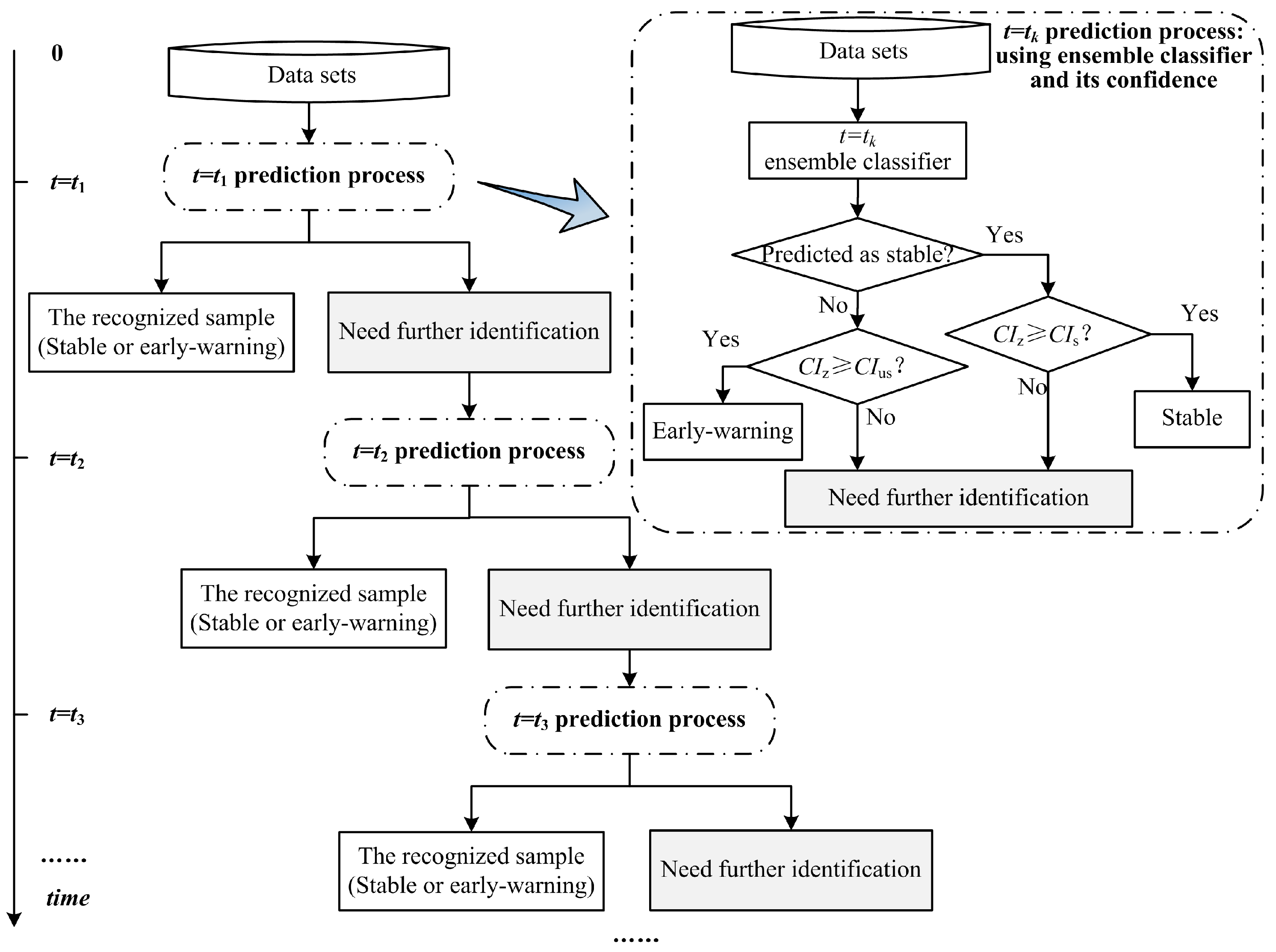
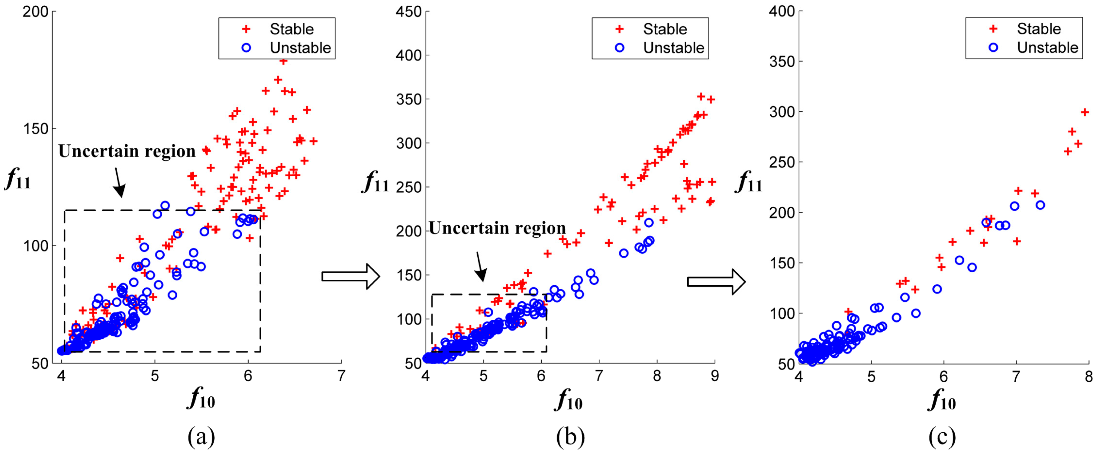
4. Proposed Hierarchical Method for Transient Stability Prediction

The dataset generation had been introduced in Section 2. In Table 1, the features f₅–f₃₄ are dynamic responses of a power system after the fault clearance. These features provide more information about the system, but require a large response time. Since the transient stability is a very fast phenomenon that demands a corrective action within short period of time (<1 s) [13], the sooner the prediction is completed, the longer the time available to take countermeasures to prevent a possible collapse will be. However, the classifier using shorter response time may not be as accurate and robust as the classifier using a longer response time. Actually, it is hard to draw a definite conclusion about how long the best response time for any power system should be. In previous research, one common way is to select a relative optimal response time by comparison among the accuracies using different response times. It can be said that the aforementioned selection of response time makes a compromise between accuracy and speed.

Considering the selection of response time and the balance between accuracy and speed of transient stability prediction, the separability of the instances with different response time is studied first. Figure 10 shows the feature space of f₁₀ versus f₁₁ using some instances in Section 5.1 at different response times after the fault clearance. Figure 10a shows the feature space at t = 0.0167 s (one sampling period for 60 Hz system) after the fault clearance. There are many overlaps among the stable and unstable instances that are difficult to separate. The overlapping region can be called the uncertain region and the instances in uncertain region are uncertain instances. Figure 10b shows that there are fewer uncertain instances at t = 0.5 s, and when t = 1 s, the uncertain instances are rare (shown in Figure 10c).

There are both certain instances and uncertain instances in the feature space at each response time. The instances far away from the stable boundary are easier to identify even at very short response times. As the response time increases, the separability of feature space is improved. Thus the uncertain instances at shorter response time will become certain instances at longer response times.

Different from the previous research, our proposed confidence index of the SVM-based ensemble classifier provides a new way to deal with the transient stability prediction. The confidence index reflects the credibility of a prediction result. If the value of confidence is high enough, the prediction result can be considered as credible, otherwise the instance should be considered as uncertain. More and more information will be obtained as the prediction process goes on. When the confidence of the prediction result reaches a preset value or threshold value, the prediction result will be accepted.

Based on the above analysis, a hierarchical scheme is proposed for transient stability prediction, shown in Figure 11. In this hierarchical scheme, multiple classifiers with different response times constitute the different layers, or levels for transient stability prediction. For an ensemble classifier at t = t₁, if an instance is predicted as stable, only when CI_Z ≥ CI_s will this instance be determined as stable. If an instance is predicted as unstable, only when CI_Z ≥ CI_us will the early-warning be carried out. The values of CI_s and CI_us are manually set. Those instances with lower confidence of prediction results will be identified as uncertain and need further identification. The instances far away from the boundary will be identified at the first layer with short response time, which ensures the rapidity. For those uncertain instances, more credible prediction results will be provided with longer response time, which ensures the accuracy. Therefore this hierarchical prediction scheme is a good solution to balance the rapidity and accuracy.

Parameters such as CI_s, CI_us and t_i need to be determined. If a stable instance is false-alarmed, there is little impact on the power system security because the emergency control measures always make the power system strong. But if an unstable instance is misjudged as stable, it would be a disaster when nothing has been done to prevent the collapse. We can image that the situation of an unstable instance identified as uncertain is more acceptable than misjudgment, because a more reliable result will be provided after some time. Therefore CI_s is set at a larger value whereas CI_us is smaller, which reduces the number of misjudgments and uncertain of unstable instances as many as possible. For the selection of t_k, t₁ is the shortest response time. The value of t₁ is set as 0.0167 s because the sampling period of response data is 0.0167 s for a 60 Hz power system. The other response times can be determined free according to actual situations.

5. Results and Discussion

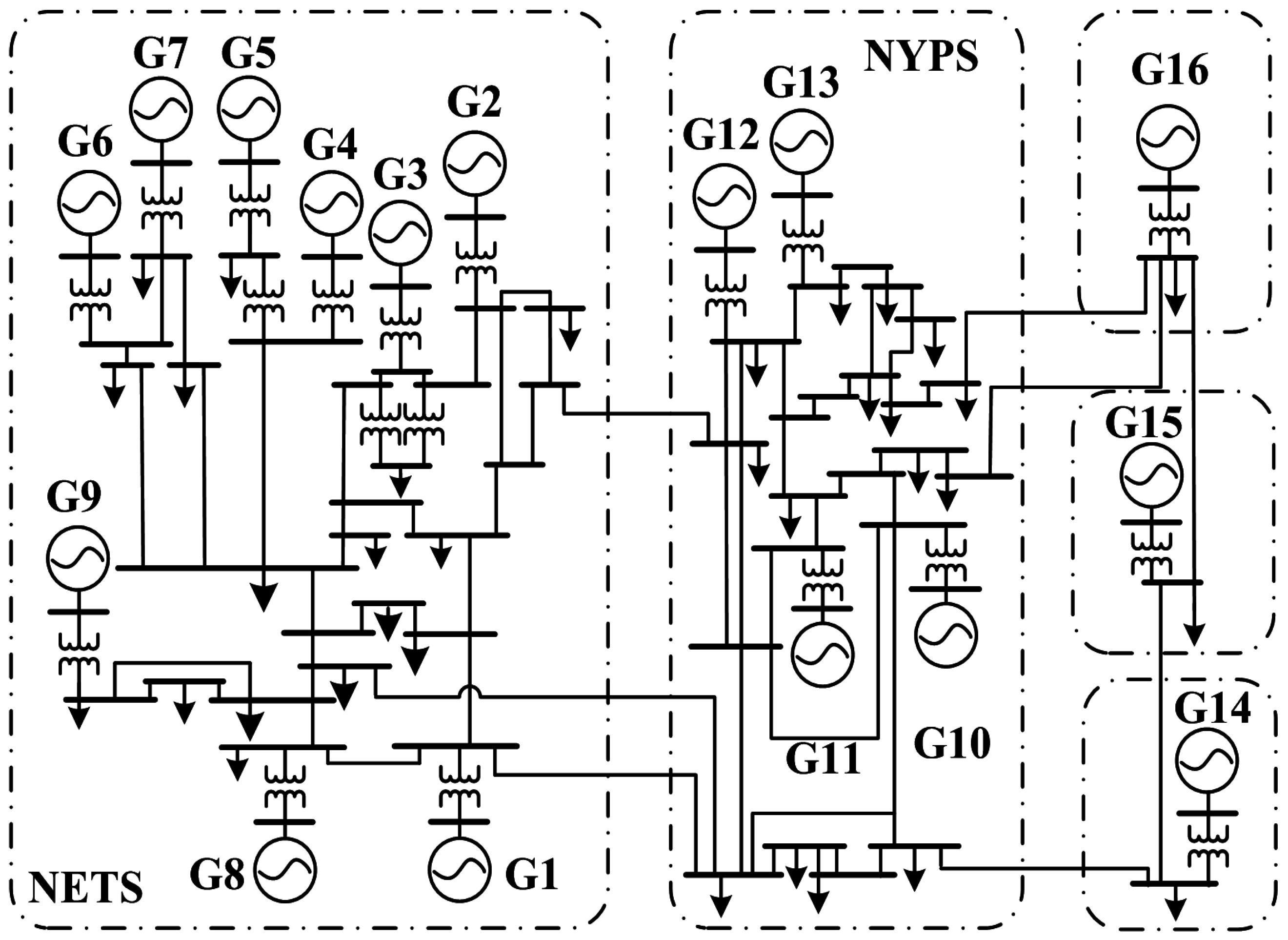
5.1. Data Generation

The test system chosen in this research is the 16-machine 68-bus reduced order equivalent model of the New England Test System and the New York Power System (NETS and NYPS), shown in Figure 12. Detailed parameters of this system can be found in [25]. The system frequencies are 60 Hz.

To generate the original data, ten load levels from 75% to 120% with an increment of 5% are used, and five kinds of generator output powers are randomly set under each load level. This process will generate 50 operating conditions of this test system. Three-phase short circuit faults at all the transmission lines are considered. Two fault clearing times, 0.1 s and 0.167 s, are assumed for all the contingencies. Considering the action of backup relay protection, an addition fault clearing time, 0.334 s, is also considered. Here, the criterion for transient stability is whether the difference between any two generator rotor angles exceeds 360 degrees [19]. It is noted that the stability criterion is dependent on the power system characteristics [8], and in this research 4 s after the fault clearance is considered as the time period of this criterion. All the transient stability simulations are carried out using the Power System Toolbox 3.0 [26], a MATLAB toolbox for power system dynamics and control. In all, 12,900 simulation instances are generated, of which 6739 instances are stable, and the remaining 6161 instances are unstable.

5.2. Performance Evaluation Method of Transient Stability Classifier

5.2.1. Cross Validation

The original dataset is usually randomly partitioned into two subsets, a training set and a testing set. The machine learning classifier will be built using the training set, and the instances in the testing set are used to validate the trained classifier.

The common validation methods include simple and cross validation. The simple validation is to randomly select some instances to generate the training dataset and the rest as the testing instances. However the randomness will influence the validation results.

Cross validation is more robust to evaluate the performance of any classifier. In this method, data are split into K partitions of approximately equal size [13]. Selecting one partition for testing and the rest K-1 partitions for training each time. This process is repeated K time and all these K partitions have been used as testing sets. Cross validation can eliminate the impact of random sampling, and the evaluation results are more persuasive. In this research, a 5-fold cross validation is utilized.

5.2.2. Indices for Performance Evaluation

The classification performance is evaluated by the following indices [27]:

(1)

Accuracy: (Number of instances − Number of misjudged instances)/Number of instances.

(2)

Reliability: (Number of unstable instances − Number of unstable instances judged as stable)/Number of unstable instances.

(3)

Security: (Number of stable instances − Number of stable instances judged as unstable)/Number of stable instances.

As mentioned earlier, the costs of misclassification of unstable instances are huge and unacceptable for online application. Thus we select the reliability as the primary index when evaluating the classifier performance. The accuracy is the most commonly used index and will also be a reference. Besides, the value of security cannot be too low because the excessive false alarms will trigger the emergency control frequently. Under this evaluation criterion, we hope the best ensemble classifier should reduce the misjudgment of the unstable instances as much as possible with affordable control costs.

5.3. Simulation Results

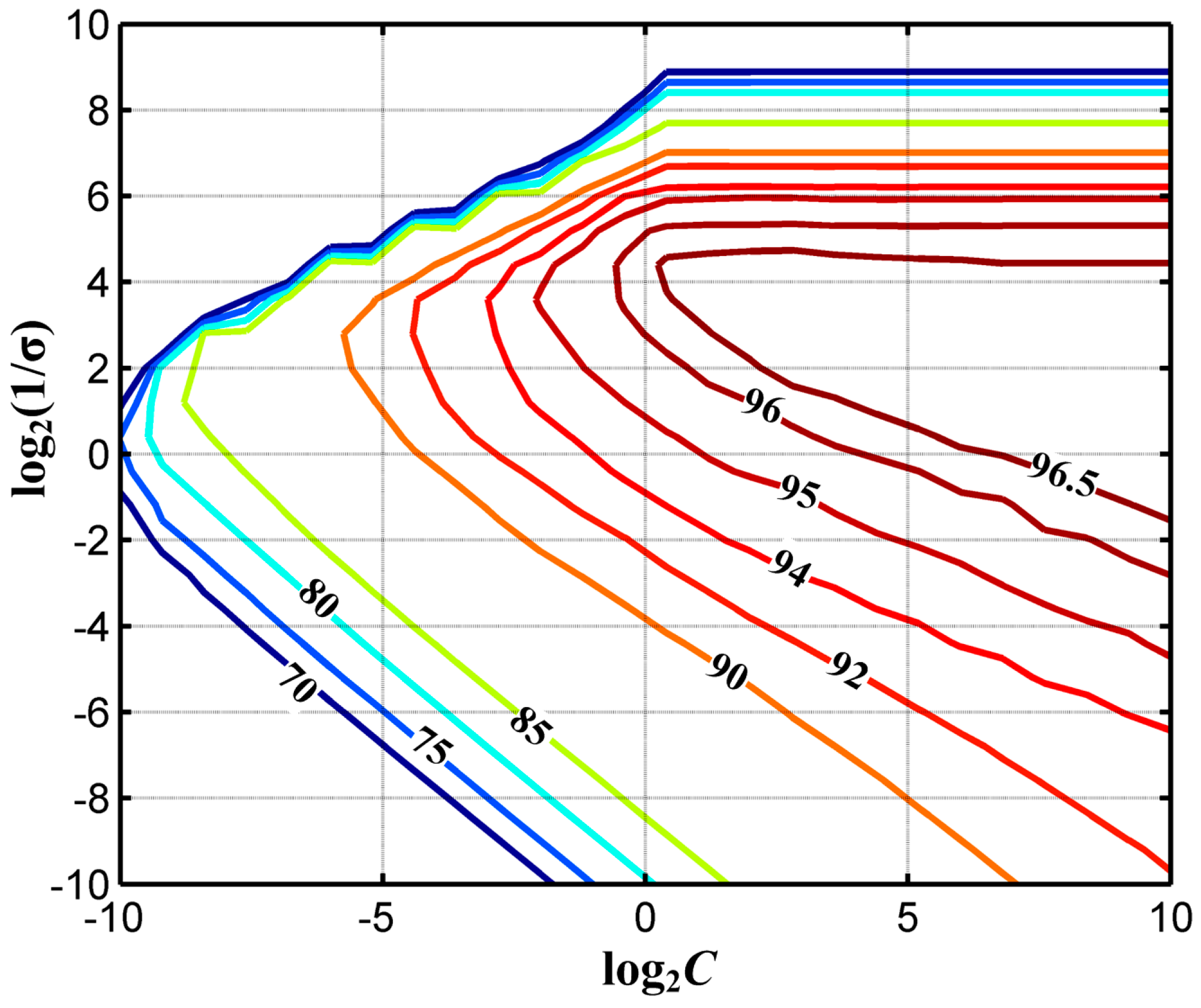
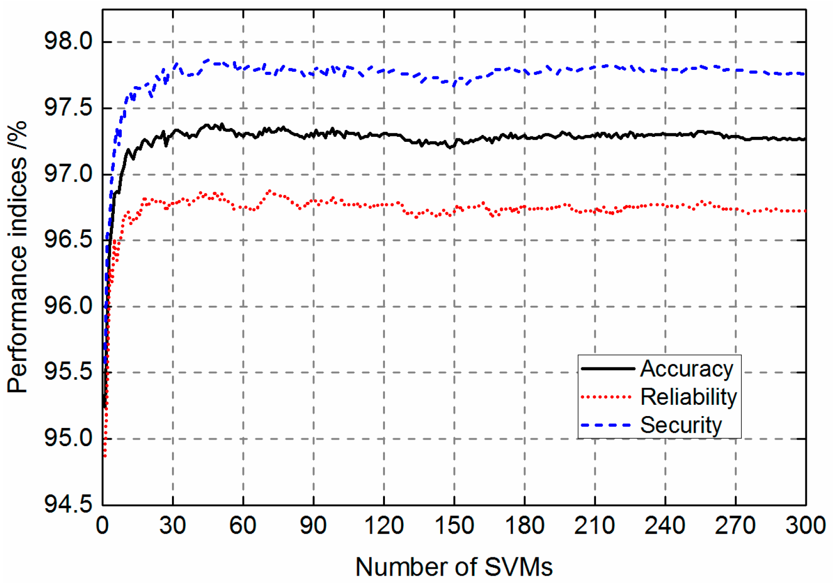
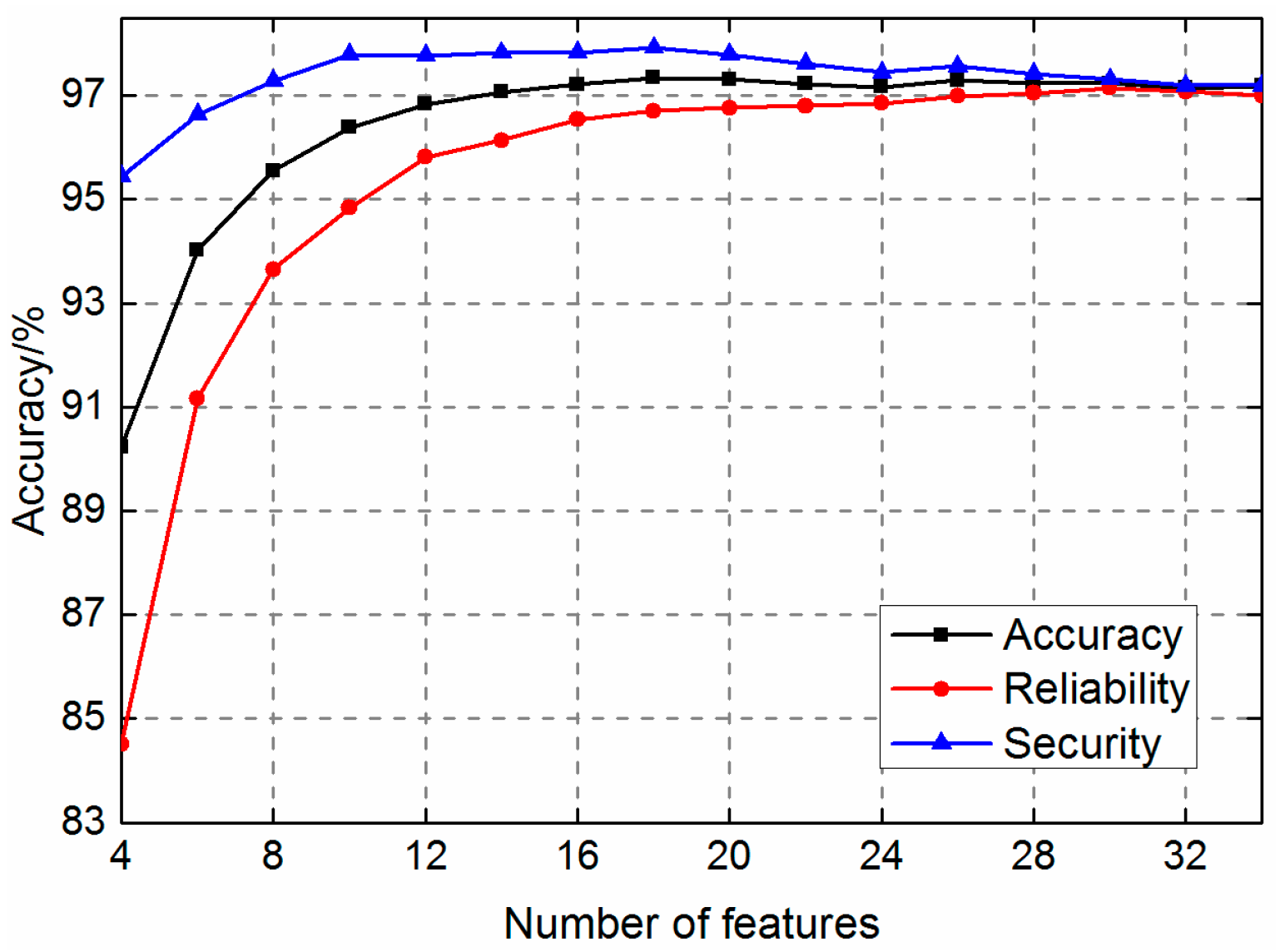
5.3.1. Parameter Determination

To build the SVM-based ensemble classifier, the number of selected features and SVMs, s and k, should be determined. Firstly, set the number of selected features s = 20 (nearly 60% features are selected), then the reliability, accuracy and security of the ensemble classifier using different numbers of SVMs are shown in Figure 13 (the response time t_k = 0.0167 s).

The values of these three evaluation indices obviously increase with the increase of number of SVMs when k < 30. When k ≥ 30, these indices reach relative constant values. The more SVMs are used, the longer the calculation time needed, therefore only 30 SVMs are used to construct the SVM-based ensemble classifier in this research. After the number of SVMs is determined, different number of features are randomly picked up to build different ensemble classifiers. The simulation results are shown in Figure 14.

Figure 14 shows that the performance of SVM-based ensemble classifiers using more than 16 features are all satisfactory. Selecting too many features will increase the computational burden, and because of the lack of diversity, the performance of the ensemble classifier using total 34 features become worse. In this research, the number of SVMs is set to 30, and the number of features in each sub-classifier is set to 20.

5.3.2. Performance Evaluation

To verify the effectiveness of the proposed SVM-based ensemble classifier, another five classifiers are generated using different machine learning techniques: DT based on C5.0, C5.0 using boosting technique, random forest (RF), extreme learning machine (ELM) and single SVM using grid-search process. The C5.0 DT and C5.0 using boosting technique are built with IBM SPSS Modeler 14.1 [9,19]. The LIBSVM toolbox [28], which is an open source MATLAB library for SVM, is used to generate all the SVM models. The RF and ELM are built using MATLAB. The tree number of RF is set to 300. The optimal parameters of single SVM and ELM are searched using a grid-search and cross validation process. All these schemes are run on a PC with an Intel Core i7-4790 3.6-GHz processor and 16 GB of RAM. Among these classifiers, the RF, Boosting C5.0 and the proposed SVM-based ensemble classifier are the ensemble models. Although these ensemble models take longer to provide prediction results [19], the order of computation time for one instance is still 10⁻³ s in this research. When using the parallel computing technique, the computation time can be further reduced.

Table 2. Performance of different classifiers. DT: decision tree; ELM: extreme learning machine; RF: random forest.

Classifier	Accuracy (%)	Reliability (%)	Security (%)
C5.0 DT	95.02	94.90	95.13
ELM	95.23	93.51	96.81
Boosting C5.0	96.76	95.97	97.48
RF	96.94	96.25	96.25
Single SVM	96.94	96.72	97.14
Proposed Method	97.31	96.77	97.79

shows the performance of different classifiers using the response time t_k = 0.0167 s.

The comparison of different classifiers indicates that among all the classifiers applied, the C5.0 DT and ELM methods perform worse since their evaluation indices are lower. The proposed SVM-based ensemble classifier performs the best since its reliability, accuracy and security are the highest. In order to demonstrate the effectiveness and necessity of using the proposed 34 features, including the generator electromagnetic powers, rotor angle dependent variables etc., the six classifiers in Table 2 with only the generator rotor angles as inputs are trained. The accuracies and reliabilities of these classifiers are lower than 88% and 81% respectively. This clearly indicates that using the proposed 34 features can make the classifier possesses better performance.

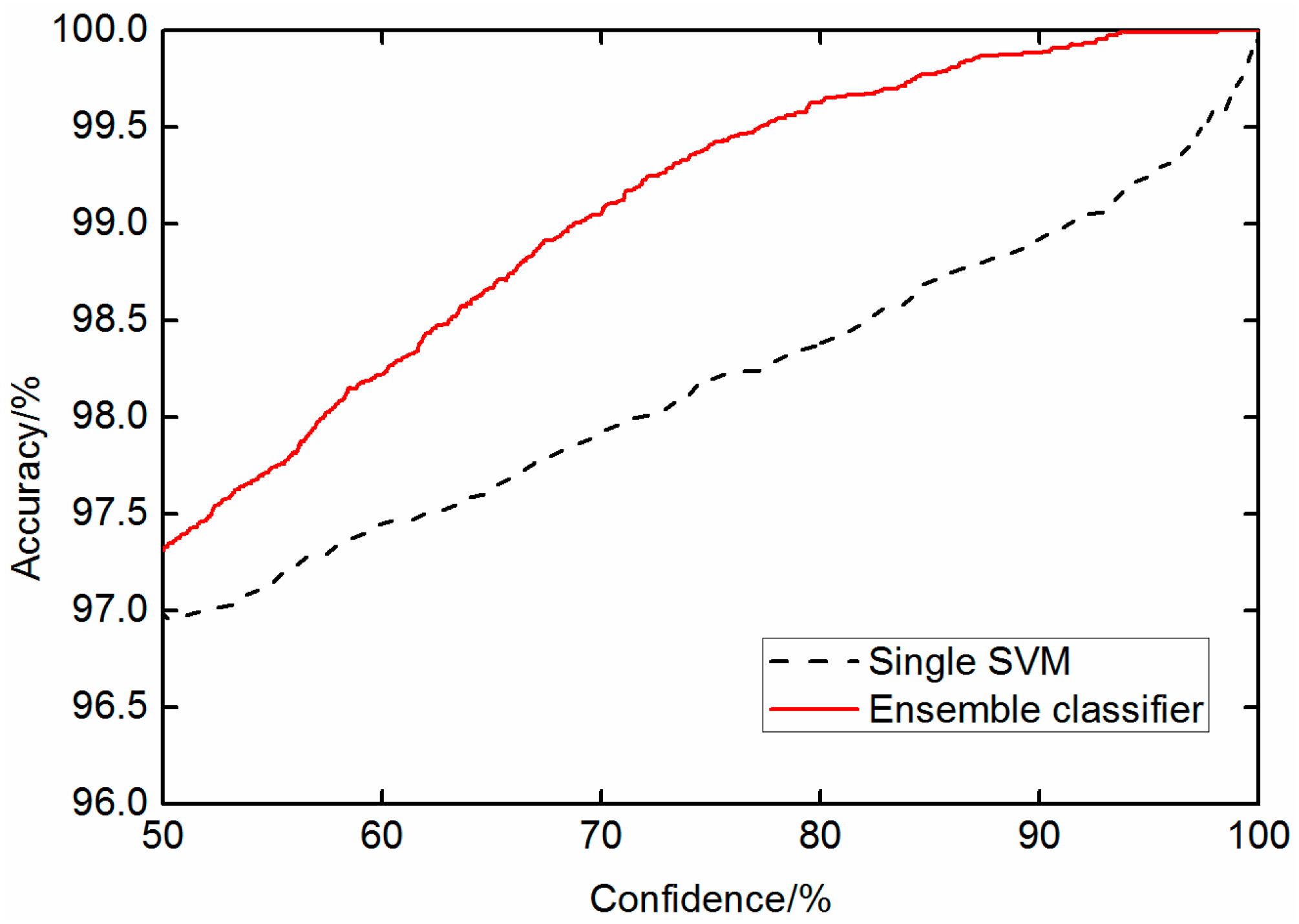
5.3.3. Confidence Evaluation

One innovation of this research is the definition of confidence index, which based on the distance between instances and SVM decision boundary. To investigate the confidence of the individual SVM and SVM-based ensemble classifiers, the “Confidence-Accuracy” curves are plotted and shown in Figure 15.

In Figure 15, the horizontal axis is the confidence, e.g., CI = x. The vertical axis is the accuracy of the instances with CI ≥ x. The trends of curves in Figure 15 indicate that the prediction results with higher confidence are more accurate. The “confidence-accuracy” curve of the SVM-based ensemble classifier is always higher than the individual SVM classifier. Besides, the accuracy of individual SVM cannot reach 100% even if the confidence is almost 100%. However, the accuracy of the instances with CI ≥ 98.12%, which includes 8234 instances, is 100% for our proposed SVM-based ensemble classifier. Therefore the proposed ensemble classifier is more reliable.

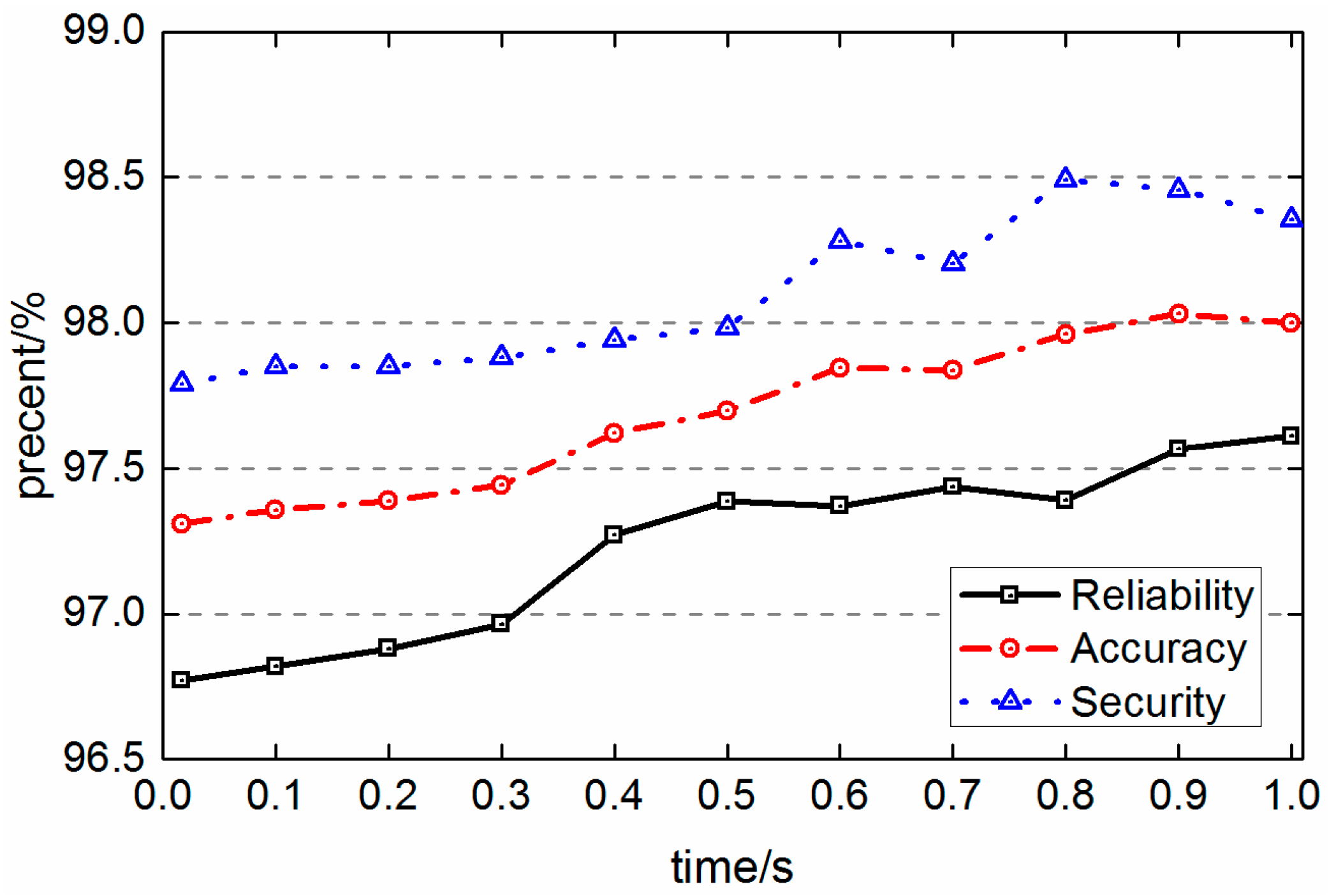
5.3.4. Hierarchical Method for Transient Stability Prediction

The above simulation results illustrate the better performance of SVM-based ensemble classifier, which lays a good foundation for the following hierarchical method. Before using the hierarchical method, the performance of different ensemble classifiers using different response time is tested, as shown in Figure 16.

Figure 16 shows that the performance of ensemble classifier is better when using a longer response time. To balance the rapidity and accuracy of transient stability prediction, the hierarchical method in Section 4 is used. The response time of the first layer is set to 0.0167 s, which is fixed in order to ensure the rapidity. The other response time, t₂ = 0.2 s, t₃ = 0.4 s, t₄ = 0.6 s, can be adjusted in different situations. To reduce the misjudgment and uncertain of unstable instances, set CI_s = 98.5% and CI_us = 60%. The prediction results are shown in

Table 3. Prediction results of the hierarchical method.

Response Time	Classified as Stable		Classified as Unstable		Uncertain Instances
	Total	Misdetection	Total	False-Alarm
t1 = 0.0167 s	3821	0	5973	92	3106
t2 = 0.2 s	685	0	105	25	2316
t3 = 0.4 s	287	0	44	14	1985
t4 = 0.6 s	170	0	30	7	1785
…	…	...	...	…	…

.

The data in the first row of Table 3 indicate that in total 9794 instances (about 75.92% instances) are identified at the first layer, of which 92 instances are false-alarms and none of unstable instances is misjudged as stable. After the screening of the first layer at t₁ = 0.0167 s, there are 3106 uncertain instances need to be further identified. At the second layer at t₂ = 0.2 s, 790 more instances are identified and the remaining 2316 uncertain instances need to be further identified. Therefore, the number of uncertain instances become less and less after the screening of multiple layers. It can also be found that none of unstable instances is misjudged, which indicates that the proposed method is more reliable.

In Table 3, there still remain 1785 uncertain instances after t₄ = 0.6 s, of which 147 instances are unstable. That means 147 unstable instances are uncertain 0.6 s after the fault clearance. The quantity is a little more and seems unsatisfactory. To further study these uncertain unstable instances, their unstability times between a fault clearance and an unstable occurrence (the difference between any two generator rotor angles exceeding 360 degrees) are counted. For the sake of comparison, the unstable time histogram of the total testing unstable instances and uncertain unstable instances are shown in Figure 17.

In Figure 17a, the red line is the maximum vertical axis value in Figure 17b. Figure 17a shows that majority of unstable instances in the total dataset have shorter unstability times. Figure 17b shows that the losses of synchronization of the remaining uncertain unstable instances always happen after 1 s. It can be said that these instances with longer unstable time are always the critical unstable instances with a multi-swing transient process. It is very difficult to identify those instances accurately and quickly with the existing approaches. The longer the unstable time is, the longer the time reserved for emergency control is. It is difficult to classify these critical instances with longer unstable time correctly, but it is more reasonable to identify these instances as uncertain ones temporarily rather than to provide wrong prediction results. The proposed method can rapidly filter out large amounts of instances far away from the classification boundary. More importantly, the setting of a confidence margin provides us a new way to reduce the misjudgments of unstable instances as much as possible. In one word, the proposed hierarchical method is more reliable and suitable for online applications.

5.4. Discussion

5.4.1. The Construction and Selection of Input Features

The reasonability of the input features has a great influence on the performance of a transient stability classifier. Currently, there is substantial research on machine learning-based methods for transient stability prediction. The construction of input features depends on researchers’ comprehension of transient stability, and the input features are different in different studies. Therefore, there is not a universal feature set to predict the transient stability.

In this research, all 34 features in Table 1 are utilized as the inputs. The number of input features is independent from the scale of the power system. This characteristic makes the proposed features more applicable for a large scale power system with hundreds or thousands of generators. However it is still necessary to verify whether the performance of the classifier using the proposed 34 features can satisfy the requirements for a large power system. Moreover, when new progress has been achieved in the mechanism of transient stability, new features should be utilized as the inputs of the machine learning-based method. On the other hand, how to select an optimal feature subset with minimum amount to generate a classifier with better performance, or the problem of feature selection, is also a key issue would be considered in the future.

5.4.2. The Communication Delay and Computation Time

For online application, the data measurements needed in the proposed method can be obtained by the wide area measurement system. However, communication link delays may occur when transferring the measurements from a remote location to the control center. The time delay can vary from tens to several hundred milliseconds or more in large-scale power systems [29]. Some measurements, which may be the input data required by the classifier, cannot reach the control center in time when the communication delay is too long. Therefore, the transient stability prediction process would be quite time-consuming or even unavailable under this condition.

One method to reduce this effect is to predict the delayed measurements based on the obtained measurements. For example, the generator valuables may present a linear or sinusoidal change tendency with time in a short period, therefore the unavailable measurements can be predicted by function fitting. As long as the prediction precision is high enough, it can reduce the influence of the time delay on transient stability prediction. Besides, new classification methods are also proposed in [30,31] to make the classifier adaptable to incomplete measurements.

The computation time, including the data pre-processing, the computation time of the input features and the classifier, is also an important issue for real-time application. In this research, the order of computation time for one instance is 10⁻³ s, which is satisfactory but will increase for large-scale power systems. Parallel computation techniques can be used to reduce the online computation time and make the proposed method more applicable.

5.4.3. The Instance Selection Problems

The instance number of the 16-machine 68-bus system in Section 5.2 is 12,900. The instance numbers in some articles were more than 90,000 [17,27]. The more the instances trained, the greater the computation time taken. However, not all the instances are useful for the training process, and there are also redundant instances that should be reduced. In fact, the instance selection is a common problem in the research of machine learning, or data mining, and many solutions have been proposed [32]. If some instances can be filtered out before the classifier training process, the efficiency of training process can be improved. These problems would not affect the comparison results in this research, but would be attached more importance in the future.

5.4.4. The Role of Machine Learning-Based Method

Historically, the research about transient stability is rich. Time domain simulation is regarded as the most accurate method. It usually acts as the calibration method of transient stability analysis. However, it is time consuming and hard to achieve online application. Actually, with the development of parallel computation and the improvement of computation speed, the computation time of time domain simulation can be reduced and even realize faster-than-real-time simulation. For instance, the simulation time can be reduced to 85.7% of the real process time by using the parallel computation [33]. That means when a power system shows an unstability at 1 s, the simulation results will be provided at 0.857 s. For different situations, the simulation time can be even further reduced.

For the proposed hierarchical method based on machine learning technique, it is NOT a replacement but an addition to time domain simulation. The hierarchical method can provide results 0.0167 s after the fault clearance, which is fast and can filter out many instances far away from the stable boundary. The next layer will continue identifying the remaining uncertain instances in the prior layer, but this process does not need to keep on all the time. When the time domain simulation provide a prediction result, e.g., for those multi-swing unstable instances, the hierarchical prediction process should be stopped and the final prediction result will be the time domain simulation result.

6. Conclusions

A hierarchical method for transient stability prediction based on the confidence of a SVM-based ensemble classifier is proposed in this paper. Firstly, multiple subsets are generated by bootstrap sampling, and the datasets are reduced by randomly picking up features. Secondly, multiple SVM classifiers are built by these datasets and features, the final ensemble classifier combined by all these SVM classifiers can provide more accurate and reliable prediction results and their confidences. Finally, different ensemble classifiers can be built using the data with different response time, and these ensemble classifiers construct different layers of the proposed hierarchical scheme. Based on the comparisons among different methods on 16-machine 68-bus system, following conclusions can be made:

(1)

The proposed SVM-based ensemble classifier can provide more accurate prediction results; most importantly, the confidence index proposed in this paper can indicate the credibility of the prediction results, and the SVM-based ensemble classifier possesses a higher confidence level.

(2)

The proposed hierarchical method can balance the accuracy and speed of the transient stability prediction. It can provide accurate results of those instances far away from the stable boundary immediately after the fault is cleared. By identification of successive layers with longer response times, more and more uncertain instances are identified with high credibility. The hierarchical method can reduce the misjudgments of unstable instances as much as possible and cooperate with the time domain simulation to insure the security and stability of power systems.

References

1. Kundur, P.; Paserba, J.; Ajjarapu, V.; Andersson, G.; Bose, A.; Canizares, C.; Hatziargyriou, N.; Hill, D.; Stankovic, A.; Taylor, C.; et al. Definition and classification of power system stability. IEEE Trans. Power Syst. 2004, 19, 1387–1401. [Google Scholar]
2. Xu, Y.; Dong, Z.Y.; Zhao, J.H.; Zhang, P.; Wong, K.P. A reliable intelligent system for real-time dynamic security assessment of power systems. IEEE Trans. Power Syst. 2012, 27, 1253–1263. [Google Scholar] [CrossRef]
3. Xu, Y.; Dong, Z.Y.; Guan, L.; Dong, Z.Y. Preventive dynamic security control of power systems based on pattern discovery technique. IEEE Trans. Power Syst. 2012, 27, 1236–1244. [Google Scholar] [CrossRef]
4. Liu, C.X.; Sun, K.; Rather, Z.H.; Chen, Z.; Bak, C.L.; Thøgersen, P.; Lund, P. A systematic approach for dynamic security assessment and the corresponding preventive control scheme based on decision trees. IEEE Trans. Power Syst. 2014, 29, 717–730. [Google Scholar] [CrossRef]
5. Luo, F.; Dong, Z.Y.; Chen, G.; Xu, Y.; Meng, K.; Chen, Y.Y.; Wong, K. Advance pattern discovery-based fuzzy classification method for power system dynamic security assessment. IEEE Trans. Power Syst. 2015, 11, 416–426. [Google Scholar]
6. Liu, C.W.; Su, M.C.; Tsay, S.S.; Wang, Y.J. Application of a novel fuzzy neural network to real-time transient stability swings prediction based on synchronized phasor measurements. IEEE Trans. Power Syst. 1999, 14, 685–692. [Google Scholar]
7. Sawhney, H.; Jeyasurya, B. A feed-forward artificial neural network with enhanced feature selection for power system transient stability assessment. Electr. Power Syst. Res. 2006, 76, 1047–1054. [Google Scholar] [CrossRef]
8. Amjady, N.; Mahedi, S.F. Transient stability prediction by a hybrid intelligent system. IEEE Trans. Power Syst. 2007, 22, 1275–1283. [Google Scholar] [CrossRef]
9. Guo, T.Y.; Milanović, J.V. Probabilistic framework for assessing the accuracy of data mining tool for online prediction of transient stability. IEEE Trans. Power Syst. 2014, 29, 377–384. [Google Scholar] [CrossRef]
10. Amraee, T.; Ranjbar, S. Transient instability prediction using decision tree technique. IEEE Trans. Power Syst. 2013, 28, 3028–3037. [Google Scholar] [CrossRef]
11. Li, M.Y.; Pal, A.; Phadke, A.G.; Thorp, J.S. Transient stability prediction based on apparent impedance trajectory recorded by PMUs. Int. J. Electr. Power Energy Syst. 2014, 54, 498–504. [Google Scholar] [CrossRef]
12. Rajapakse, A.D.; Gomez, F.R.; Nanayakkara, K.; Crossley, P.A.; Terzija, V.V. Rotor angle instability prediction using post-disturbance voltage trajectories. IEEE Trans. Power Syst. 2010, 25, 947–956. [Google Scholar] [CrossRef]
13. Gomez, F.R.; Rajapakse, A.D.; Annakkage, U.D.; Fernando, I.T. Support vector machine-based algorithm for post-fault transient stability status prediction using synchronized measurements. IEEE Trans. Power Syst. 2011, 26, 1474–1483. [Google Scholar] [CrossRef]
14. You, D.; Wang, K.; Ye, L.; Wu, J.; Huang, R. Transient stability assessment of power system using support vector machine with generator combinatorial trajectories inputs. Int. J. Electr. Power Energy Syst. 2013, 44, 318–325. [Google Scholar] [CrossRef]
15. Geeganage, J.; Annakkage, U.D.; Weekes, T.; Archer, B.A. Application of energy-based power system features for dynamic security assessment. IEEE Trans. Power Syst. 2015, 30, 1957–1965. [Google Scholar] [CrossRef]
16. Abdelaziz, A.Y.; Abbas, A.A.; Naiem, A.F.; Elsharkawy, M.A. Transient stability assessment using an adaptive fuzzy classification technique. Electr. Power Compon. Syst. 2006, 34, 927–940. [Google Scholar] [CrossRef]
17. Kamwa, I.; Samantaray, S.R.; Joós, G. Development of rule-based classifiers for rapid stability assessment of wide-area post-disturbance records. IEEE Trans. Power Syst. 2009, 24, 258–270. [Google Scholar] [CrossRef]
18. Dora Arul Selvi, B.; Kamaraj, N. Transient stability assessment using fuzzy combined support vector machines. Electr. Power Compon. Syst. 2010, 38, 737–751. [Google Scholar] [CrossRef]
19. Guo, T.Y.; Milanović, J.V. Online identification of power system dynamic signature using PMU measurements and data mining. IEEE Trans. Power Syst. 2016, 31, 1760–1768. [Google Scholar] [CrossRef]
20. Fang, D.Z.; David, A.K. A normalized energy function for fast transient stability assessment. Electr. Power Syst. Res. 2004, 69, 287–293. [Google Scholar] [CrossRef]
21. Cherkassky, V.S.; Mulier, F. Learning from Data: Concepts Theory and Method, 2nd ed.; IEEE Press: Hoboken, NJ, USA, 2007. [Google Scholar]
22. Hartman, E.J.; Keller, J.D.; Kowalski, J.M. Layered neural networks with Gaussian hidden units as universal approximations. Neural Comput. 1990, 2, 210–215. [Google Scholar] [CrossRef]
23. Platt, J.C. Probabilistic output for support vector machine and comparisons to regularized likelihood methods. In Advances in Large Margin Classifiers; MIT Press: Cambridge, MA, USA, 1999; pp. 61–74. [Google Scholar]
24. Han, J.; Kamber, M.; Pei, J. Data Ming: Concept and Techniques, 3rd ed.; Elsevier: Amsterdam, The Netherlands, 2012; pp. 363–385. [Google Scholar]
25. Rogers, G. Power System Oscillations; Kluwer: Norwell, MA, USA, 2000; pp. 171–185. [Google Scholar]
26. Chow, J.H.; Cheung, K.W. A toolbox for power system dynamics and control engineering education and research. IEEE Trans. Power Syst. 1992, 7, 1559–1564. [Google Scholar] [CrossRef]
27. Kamwa, I.; Samantaray, S.R.; Joós, G. On the accuracy versus transparency trade-off of data-mining models for fast-response PMU-based catastrophe predictors. IEEE Trans. Smart Grid. 2012, 3, 152–161. [Google Scholar] [CrossRef]
28. Chang, C.C.; Lin, C.J. Libsvm: A library for support vector machines. ACM Trans. Intell. Syst. Technol. 2011, 2, 1–27. [Google Scholar] [CrossRef]
29. Naduvathuparambil, B.; Valenti, M.C.; Feliachi, A. Communication delays in wide area measurement systems. In Proceedings of the Thirty-Fourth Southeastern Symposium on System Theory, Huntsville, AL, USA, 18–19 March 2002; pp. 118–122.
30. Guo, T.; Milanović, J.V. The effect of quality and availability of measurement signals on accuracy of on-line prediction of transient stability using decision tree method. In Proceedings of 2013 4th IEEE/PES Innovative Smart Grid Technologies Europe (ISGT Europe), Copenhagen, Denmark, 6–9 October 2013.
31. He, M.; Vittal, V.; Zhang, J.S. Online dynamic security assessment with missing PMU Measurements: A data mining approach. IEEE Trans. Power Syst. 2013, 28, 1969–1977. [Google Scholar] [CrossRef]
32. Chen, J.; Zhang, C.; Xue, X.; Liu, C.L. Fast instance selection for speeding up support vector machines. Knowl.-Based Syst. 2013, 45, 1–7. [Google Scholar] [CrossRef]
33. Jiang, Q.Y.; Jiang, H. OpenMP-based parallel transient stability simulation for large-scale power systems. Sci. China Technol. Sci. 2012, 55, 2837–2846. [Google Scholar] [CrossRef]
Figure 1. Dataset for machine learning-based transient stability prediction.
Energies 09 00778 g001
Figure 2. The variation of Pei/Pmi of 16-machine 68-bus system: (a) unstable case; and (b) stable case.
Energies 09 00778 g002
Figure 3. Generator rotor angles of 16-machine 68-bus system: (a) unstable case; and (b) stable case.
Energies 09 00778 g003
Figure 4. Generator rotor speeds of 16-machine 68-bus system: (a) unstable case; and (b) stable case.
Energies 09 00778 g004
Figure 5. Generator rotor accelerations of 16-machine 68-bus system: (a) unstable case; and (b) stable case.
Energies 09 00778 g005
Figure 6. Generator kinetic energy of 16-machine 68-bus system: (a) unstable case; and (b) stable case.
Energies 09 00778 g006
Figure 7. Principle of support vector machine (SVM): (a) original data; and (b) transformed data.
Energies 09 00778 g007
Figure 8. The confidence index of SVM versus g(x).
Energies 09 00778 g008
Figure 9. Selection results of SVM parameters.
Energies 09 00778 g009
Figure 10. Feature space of f10 versus f11 at different response time: (a) t = 0.0167 s; (b) t = 0.5 s; and (c) t = 1 s.
Energies 09 00778 g010
Figure 11. Hierarchical scheme for transient stability prediction.
Energies 09 00778 g011
Figure 12. The New England Test System and the New York Power System (NETS and NYPS).
Energies 09 00778 g012
Figure 13. Prediction results of SVM-based ensemble classifiers using different numbers of SVMs.
Energies 09 00778 g013
Figure 14. Prediction results of SVM-based ensemble classifiers using different numbers of features.
Energies 09 00778 g014
Figure 15. Confidence-Accuracy curves of different classifiers.
Energies 09 00778 g015
Figure 16. Performance of different SVM-based ensemble classifier using different response times.
Energies 09 00778 g016
Figure 17. Histogram of unstable time: (a) Total testing unstable instances; and (b) Uncertain unstable instances after tk = 0.6 s.
Energies 09 00778 g017