Article

Sensitivity-Based Model of Low Voltage Distribution Systems with Distributed Energy Resources

1
Department of Electrical and Information Engineering, University of Cassino and Southern Lazio, Via di Biasio 43, I-03043 Cassino, Italy
2
Engineering Department, Università Niccolò Cusano, I-00166 Roma, Italy
*
Author to whom correspondence should be addressed.
These authors contributed equally to this work.
Energies 2016, 9(10), 801; https://doi.org/10.3390/en9100801
Submission received: 29 July 2016 / Accepted: 19 September 2016 / Published: 4 October 2016

Abstract

:
A key issue in Low Voltage (LV) distribution systems is to identify strategies for the optimal management and control in the presence of Distributed Energy Resources (DERs). To reduce the number of variables to be monitored and controlled, virtual levels of aggregation, called Virtual Microgrids (VMs), are introduced and identified by using new models of the distribution system. To this aim, this paper, revisiting and improving the approach outlined in a conference paper, presents a sensitivity-based model of an LV distribution system, supplied by an Medium/Low Voltage (MV/LV) substation and composed by several feeders, which is suitable for the optimal management and control of the grid and for VM definition. The main features of the proposed method are: it evaluates the sensitivity coefficients in a closed form; it provides an overview of the sensitivity of the network to the variations of each DER connected to the grid; and it presents a limited computational burden. A comparison of the proposed method with both the exact load flow solutions and a perturb-and-observe method is discussed in a case study. Finally, the method is used to evaluate the impact of the DERs on the nodal voltages of the network.

1. Introduction

Existing distribution networks present an inflexible structure which makes them inadequate to allow a large spread of Distributed Energy Resources (DERs), such as distributed generators from renewable energy sources, cogeneration facilities, energy storage systems (including electric vehicles), and controllable loads (i.e., adopting active demand) [1,2,3]. To overcome this problem, the smart grid paradigm is asserted and promoted by extensive use of Information and Communication Technologies [4,5,6]. However, the advent of smart distribution grids will not take place by a revolution, because it would require expensive investments, especially for Low Voltage (LV) networks that actually present a low level of control and automation. The evolution from the present networks to the future smart grids will be progressive instead. Then, the main technical challenge is to improve the flexibility of the existing LV networks with limited investments so as to allow the wide spread of DERs and enhance the power quality of the grids [7].
In this context, a key issue is to identify strategies for the optimal management and control of the LV distribution networks in the presence of DERs. For an optimal distribution system operation, the same strategy adopted at the transmission level could be used, in which a single operator controls the whole power system by gathering measurements and acting on each electrical node of the grid. Unfortunately, if such an approach were applied to LV distribution networks, it would be technically and economically infeasible because of the need to acquire and process a huge amount of information, due to the large number of nodes and customers in the grids.
To reduce the number of variables to be monitored and controlled, an alternative approach consists of modeling each LV distribution system by a cluster of Virtual Microgrids (VMs) and building communication infrastructures among a few distributed controllers of the VMs and a control center located at the Medium/Low Voltage (MV/LV) substation. Similarly to a microgrid [8], a VM is composed of parts of the distribution networks including different types of DERs and their control systems. However, differently from a microgrid, a VM is not self sustained from an energy point of view, and it is not equipped with an autonomous centralized management and control system. To identify VMs, new models of the distribution system are required. These models must be able to overcome the classical formulation adopted at the transmission level (based on non-linear equations written for each node of the grid) so as to facilitate the aggregation of portions of network on the basis of the impact of DERs on specific control actions (i.e., voltage regulation [9,10] and current flow limitation [11]). Sensitivity analysis can help face such a problem by quantifying the dependency between nodal voltages and power flows of the grid as a linear function of both load consumptions and DERs’ absorbtions/injections.
Several methods have been proposed in literature to perform sensitivity analysis. In [9], a Jacobian-based method has been shown to control the nodal voltages by regulating the reactive powers injected by distributed generators. Voltage magnitude as well as active and reactive power-loss sensitivity coefficients for radial distribution networks have been calculated in [11] by using only a base-case load flow solution. In [12], both the Gauss–Seidel method and Z-bus matrix have been used to derive voltage and loss sensitivity coefficients as functions of real and reactive power injections. In [13], voltage sensitivity factors and a linear load flow model for LV distribution system have been derived by using historical smart meter data. In [14], sensitivities of bus voltage magnitudes to load changes have been calculated using the adjoint-network method. In [15], a perturb-and-observe algorithm has been proposed to compensate voltage rises induced by distributed generators and to test siting and sizing of capacitors. Initial studies on the application of a closed-form solution of the Dist–Flow equations of an LV distribution system have been shown in [16,17].
This paper, adopting the approach outlined in [16], proposes a sensitivity-based model of an LV distribution system supplied by an MV/LV substation and composed by several feeders, which is suitable for the optimal management and control of the grid and, then, for VM definition. Such a model provides, in a closed form, the variations of the electrical variables characterizing each node of a feeder (e.g., out-flowing active and reactive powers, nodal voltage) as linear functions of the powers injected/absorbed by each DER connected to the LV network. The key steps of the proposed model are: (i) the linearization of the branch flow equations of the electrical components of the distribution system; (ii) the use of the chain-rule; (iii) the use of the border constraints at both the MV substation busbar and the end-nodes of the feeders; and (iv) the use of the coupling equations at the LV substation busbar. The main features of the proposed method are the following: (i) it evaluates the sensitivity coefficients in a closed form; (ii) it provides an overview of the sensitivity of the network to the variations of each DER connected to the grid; and (iii) it presents a limited computational burden. The last feature is very important because of the large number of nodes in LV distribution networks, of the need to repeat the analysis when the operating conditions of the distribution system change, and of the large dimension of the optimal management problems that account for the random nature of DERs.
With respect to [16], the paper presents in more details the method derived from the model, puts it into the frame of the sensitivity analysis, compares it with other methods, and applies it to DER impact evalutation in view of VM definition. After a brief introduction, in the paper, the sensitivity-based model of the LV distribution system is recalled and the step-by-step procedure of the method is presented in Section 2; then, an extensive case study is discussed in Section 3. Firstly, different sensitivity matrices are evaluated to illustrate how the proposed model provides the response of the LV distribution system to the DERs’ injections. Then, a comparison of the proposed method with both exact load flow solution and a perturb-and-observe method is discussed. Finally, the proposed method is used to evaluate the impact of the DERs on the nodal voltages of the network so as to provide a road map to perform voltage regulation. Conclusions and further research developments are reported in Section 4.

2. Distribution System Modeling
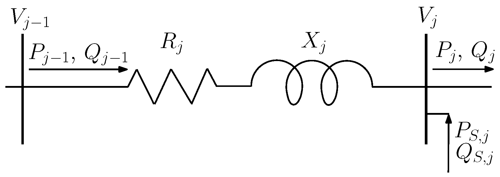
Let us consider the LV distribution system reported in Figure 1: an MV/LV substation supplies m feeders; the h-th feeder is composed of n h branches and n h + 1 nodes (node 0 is common to all the feeders being the LV busbar of the substation); along the feeders, uncontrolled loads and/or DERs can be connected. In balanced operating conditions, the MV/LV supplying system is modeled by the electric circuit shown in Figure 2. Two electric parameters identify the supplying system, namely the resistance R t r of the MV/LV transformer and the equivalent impedance X e q = X t r + X s c , where X t r is the transformer reactance and X s c the short-circuit impedance of the MV node. Three electric variables characterize the model at the supplying MV node, namely the open-circuit voltage amplitude V M V of the MV node (assumed to be fixed as the slack node), the in-flowing active power P M V and the in-flowing reactive power Q M V . Analogously, three electric variables characterize the MV/LV substation at the receiving node 0, namely the voltage amplitude V t r and the out-flowing active and reactive powers, P t r and Q t r , respectively. In a similar way, the j-th branch of a generic feeder of the LV distribution system is represented by the electric circuit shown in Figure 3. Two electric parameters identify the branch, namely the resistance R j and the reactance X j ; three electric variables characterize the branch at the supplying node j 1 , namely the voltage amplitude V j 1 , the in-flowing active power P j 1 and the in-flowing reactive power Q j 1 ; analogously, the same electric variables characterize the branch at the receiving node j, namely the voltage V j , and the out-flowing active and reactive powers, P j and Q j , respectively; in addition, other two external variables are taken into account at the receiving node j, which are the shunt active power P S , j and the shunt reactive power Q S , j defined as:
P S , j = P D E R , j P L , j , Q S , j = Q D E R , j Q L , j ,
where P D E R , j and Q D E R , j are, respectively, the active and reactive powers injected by the DER connected to the j-th node; P L , j and Q L , j are, respectively, the active and reactive powers absorbed by the uncontrolled load connected to the j-th node, which are assumed to be constant. The model of the LV distribution system, which is useful for the VM definition and which overcomes the limits of the classical formulation adopted at the transmission level (based on non-linear equations written for each node of the grid), is presented in the following. In particular, by the linearization of the branch flow equations associated with the components of the LV distribution system represented in Figure 2 and Figure 3, and by imposing both border and coupling conditions, a closed form solution of the linearized DistFlow equations is obtained through the use of the chain rule. Such a closed form represents the linear model of the distribution system with DERs, and it is expressed in terms of the variations of the electrical variables of the LV networks (with respect to an initial operating point) as linear functions of the DER injections. The model is built step by step: firstly, the model of a generic branch and of a feeder composed of different branches is developed; then, the model of the MV/LV supplying system is introduced and combined with the models of the feeders, yielding the model of the whole LV distribution system.

2.1. Branch Model

The model of the j-th branch is derived from the following steady-state branch flow equations [18]:
P j = P j 1 R j ( P j 1 2 + Q j 1 2 ) / V j 1 2 + P S , j , Q j = Q j 1 X j ( P j 1 2 + Q j 1 2 ) / V j 1 2 + Q S , j , V j 2 = V j 1 2 2 R j P j 1 + X j Q j 1 + ( R j 2 + X j 2 ) ( P j 1 2 + Q j 1 2 ) / V j 1 2 .
Since they are not linear, they can be linearized around an initial operating point of the distribution system, characterized by null powers injected by all the DERs connected to the LV distribution system and a given absorption of all the uncontrolled loads. In the following, the electrical variables evaluated in the initial operating point are identified by zero superscript.
Let the vector of nodal variables x j be defined as:
x j = P j Q j V j 2 T .
The linearization of Equation (1) yields the following branch model:
Δ x j = J j Δ x j 1 + ( Δ P S , j Δ Q S , j 0 ) T ,
Δ x j being the variation of the nodal variables x j with respect to their value x j 0 in the initial operating point
Δ x j = x j x j 0 = Δ P j Δ Q j Δ V j 2 T ,
with J j being the Jacobian matrix related to (1) evaluated in the initial operating point and Δ P S , j , Δ Q S , j the injections of the active and reactive powers by the DERs connected at the receiving node.
Equation (2) is the branch model: it expresses the vector Δ x j of the variation of the electrical variables at the receiving node x j with respect to the initial operating point x j 0 as a function of
  • the vector Δ x j 1 of the variation of the electrical variables at the supplying node x j 1 , with respect to the initial operating point x j 1 0 , through the Jacobian matrix J j ; and
  • the vector ( Δ P S , j Δ Q S , j 0 ) T of the DERs active and reactive power injections at the receiving node, which are assumed to be assigned enforcements.
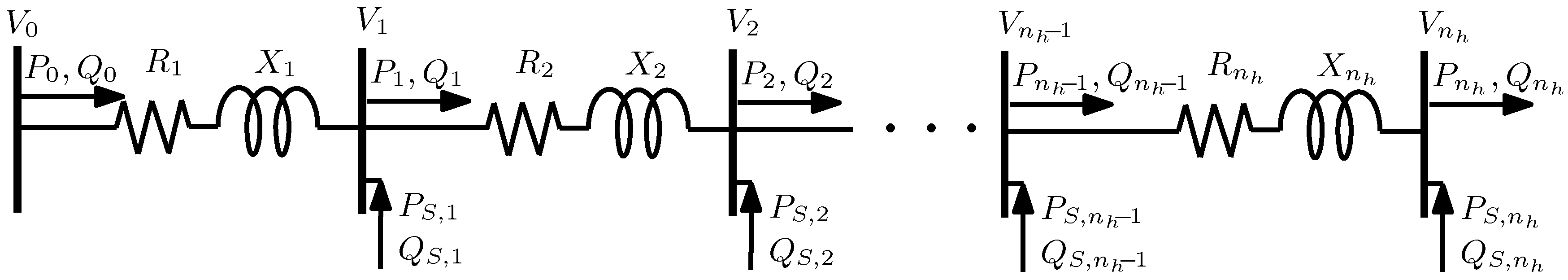
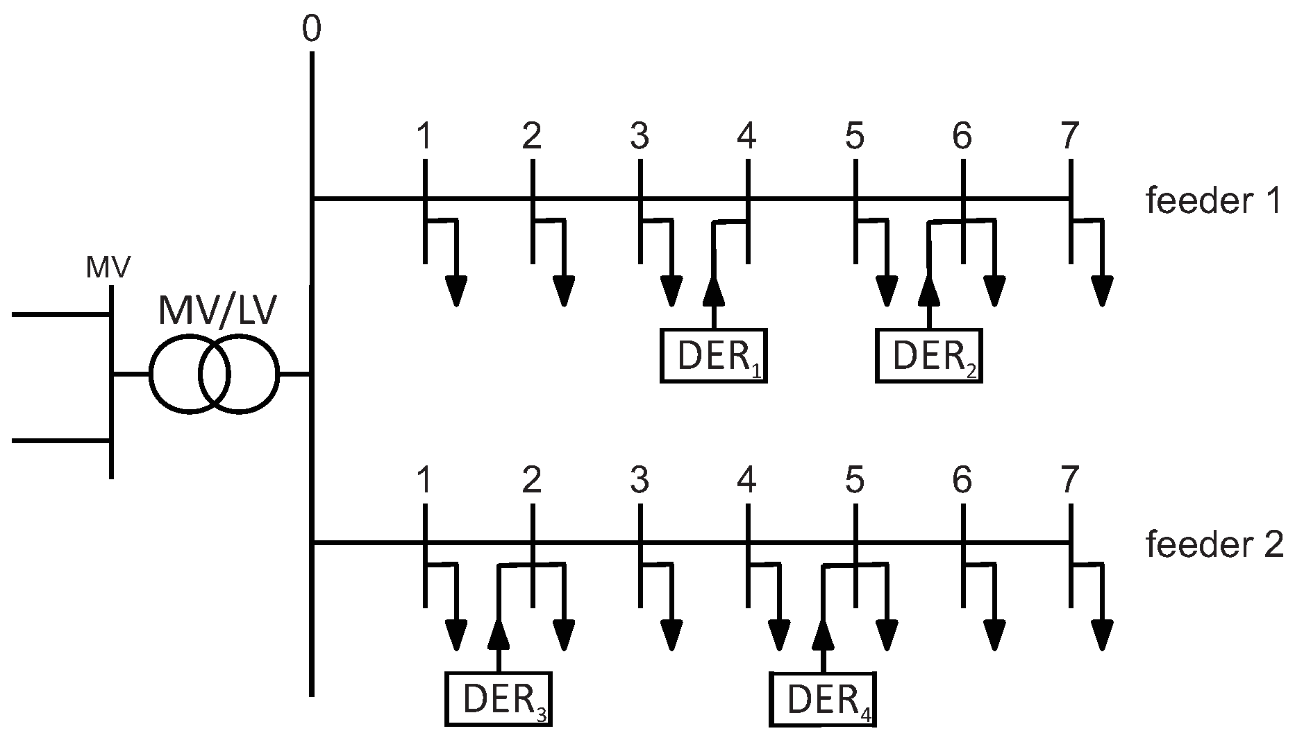
2.2. Feeder Model

The electric equivalent circuit of the h-th feeder of the LV distribution system is composed of a series of n h branches (Figure 4). Then, the model of the feeder is composed of n h equations of type (2):
Δ x j = J j Δ x j 1 + Δ P S , j Δ Q S , j 0 T ,
with j = 1 , . . . , n h .
Applying the chain rule to Equation (3),
Δ x j = M j Δ x 0 + k = 1 j N j , k ( Δ P S , k Δ Q S , k 0 ) T
is induced where
M j = = 0 j 1 J j j = 1 , , n h ,
N j , k = = 0 j k 1 J j j = 1 , , n h k = 1 , , j 1 ,
and N j , j is equal to the identity matrix I. Assuming N j , k = 0 for k > j , Equation (4) can be re-written as
Δ x j = M j Δ x 0 + k = 1 n h N j , k Δ P S , k Δ Q S , k 0 ,
with j = 1 , , n h .
Equation (7) is a set of n h equations in n h + 1 variables, which are Δ x j and Δ x 0 . To obtain a defined problem, three additional conditions must be assigned. They can be derived from the behavior of the feeder at its borders. In particular, the voltage amplitude at the head of the feeder is imposed by the MV/LV supplying substation and the active and reactive powers flowing out of the end-node of the feeder are always null. The border conditions can be expressed in terms of variations of the electric nodal variables as
Δ V 0 2 = Δ V ˜ 0 2 , Δ P n h = 0 , Δ Q n h = 0 ,
where Δ V ˜ 0 2 is the variation of the squared voltage amplitude imposed at the LV busbar by the MV/LV supplying substation. By substituting Equation (8) into Equation (7) for j = n h ,
0 0 Δ V n h 2 = M n h Δ P 0 Δ Q 0 Δ V ˜ 0 2 + k = 1 n h N n h , k Δ P S , k Δ Q S , k 0
is obtained.
The subset composed of the first two rows in Equation (9) can be solved in the two unknowns, Δ P 0 and Δ Q 0 , yielding:
Δ P 0 Δ Q 0 = k = 1 n h A ¯ k Δ P S , k Δ Q S , k + a ¯ Δ V ˜ 0 2 ,
where,
A ¯ k = M ¯ n h 1 N ¯ n h , k , a ¯ = M ¯ n h 1 m ¯ n h ,
with M ¯ n h and N ¯ n h , k the ( 2 × 2 ) leading principal minors of M n h and N n h , k , respectively, and with m ¯ n h the ( 2 × 1 ) column vector composed of the first two rows in the third column of M n h .
Combining Equation (10) with the condition on Δ V 0 2 in Equation (8), the variable Δ x 0 can be written in the form:
Δ x 0 = Δ P 0 Δ Q 0 Δ V 0 2 = k = 1 n h A k Δ P S , k Δ Q S , k 0 + a Δ V ˜ 0 2 ,
where each A k is a ( 3 × 3 ) matrix obtained by edging A ¯ k with a third row and column of zero elements, and a is a ( 3 × 1 ) vector obtained by adding a third row with a unitary element to a ¯ .
By substituting Δ x 0 given by Equation (12) into Equation (7) yields the model of the feeder:
Δ x j = k = 1 n h B j , k Δ P S , k Δ Q S , k 0 + b j Δ V ˜ 0 2 ,
with j = 1 , , n h , where:
B j , k = M j A k + N j , k , b j = M j a ,
which are, respectively, ( 3 × 3 ) matrices and ( 3 × 1 ) vectors of sensitivity with known coefficients.
In Equation (13), the vectors Δ x j of the variation of the electric variables at the receiving node of each branch belonging to the feeder are expressed as a function of:
  • The vectors ( Δ P S , k Δ Q S , k 0 ) T of the DERs active and reactive power injections in all the nodes of the feeder through the matrices B j , k ; and
  • The variation Δ V ˜ 0 2 of the squared voltage amplitude at the LV busbar of the supplying substation through the vectors b j .
To specify the model Equations (12) and (13) for each one of the m feeders, a superscript referring to the feeder number is added to the variables, matrices and vectors. Then, the model Equations (12) and (13) for the h-th feeders becomes:
Δ x 0 h = k = 1 n h A k h Δ P S , k h Δ Q S , k h 0 + a h Δ V ˜ 0 2 ,
Δ x j h = k = 1 n h B j , k h Δ P S , k h Δ Q S , k h 0 + b j h Δ V ˜ 0 2 ,
with j = 1 , , n h and h = 1 , . . . , m .

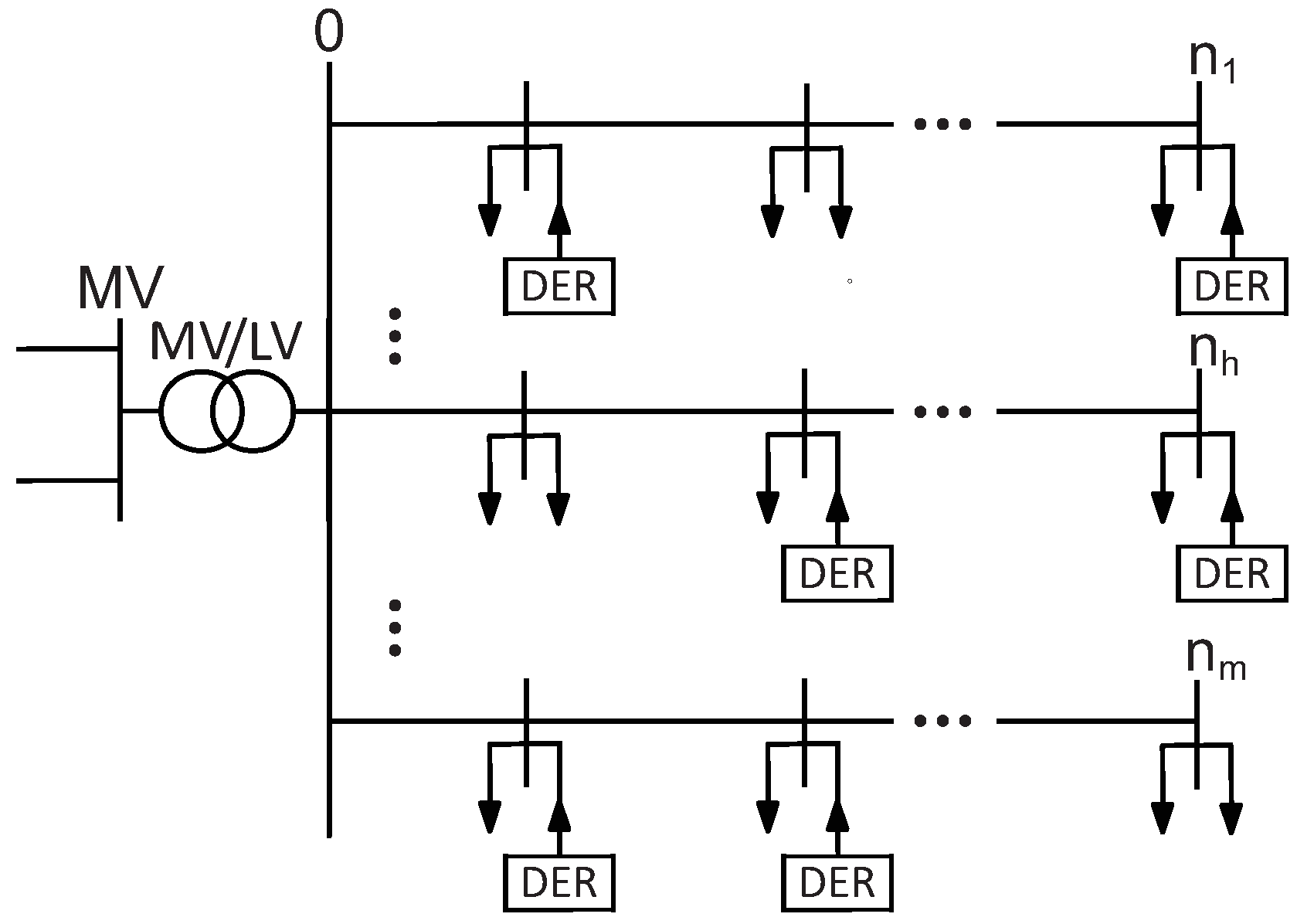
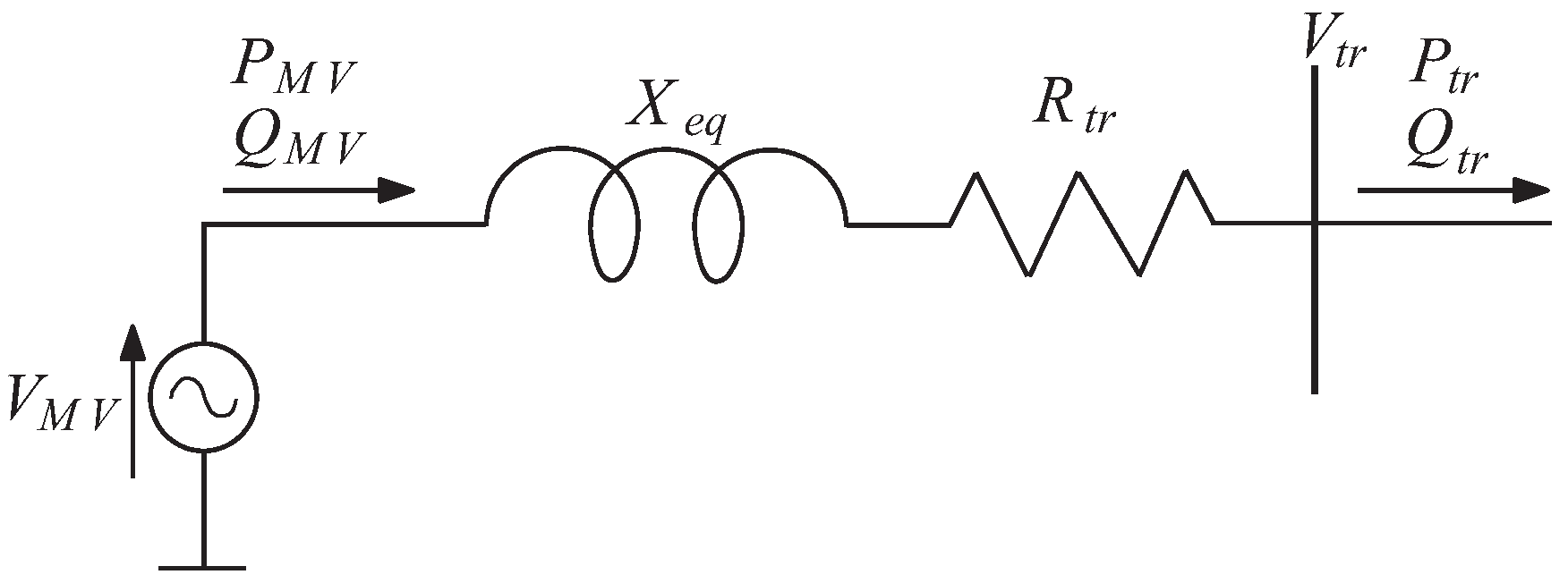
2.3. Medium/Low Voltage Supplying System

Similarly to the branch model Equation (2), the MV/LV supplying system, can be modeled as:
Δ x M V = J s u b Δ x t r ,
where:
Δ x M V = ( Δ P M V Δ Q M V 0 ) T , Δ x t r = Δ P t r Δ Q t r Δ V t r 2 T ,
where Δ V M V 2 = 0 and J s u b is the Jacobian matrix of the linearized branch flow equations of the electric circuit in Figure 2.

2.4. Low Voltage Distribution System Model

To obtain the model of the whole LV distribution system in Figure 1, it is necessary to combine the model Equation of the MV/LV supplying system (17) with the model Equations of the feeders (15) and (16).
As evident from Figure 1, three coupling equations can be written:
Δ V t r 2 = Δ V ˜ 0 2 ;
Δ P t r = i = 1 m Δ P 0 i Δ Q t r = i = 1 m Δ Q 0 i .
By substituting Equations (18) and (19) into (17),
Δ P M V Δ Q M V 0 = J s u b i = 1 m Δ P 0 i i = 1 m Δ Q 0 i Δ V ˜ 0 2
is obtained.
Substituting the expression (10) generalized for m feeders, the third equation in (20) is written as:
0 = J 3 , 3 s u b Δ V ˜ 0 2 + J 3 , 1 s u b J 3 , 2 s u b i = 1 m k = 1 n i A ¯ k i Δ P S , k i Δ Q S , k i + a ¯ i Δ V ˜ 0 2 ,
with ( J 3 , 1 s u b , J 3 , 2 s u b , J 3 , 3 s u b ) being the third row of J s u b . By solving Equation (21) in the variable Δ V ˜ 0 2 ,
Δ V ˜ 0 2 = α ¯ T i = 1 m k = 1 n i A ¯ k i Δ P S , k i Δ Q S , k i
is obtained, where α ¯ is a ( 2 × 1 ) vector equal to:
α ¯ = J 3 , 1 s u b J 3 , 2 s u b i = 1 m a ¯ i + J 3 , 3 s u b 1 J 3 , 1 s u b J 3 , 2 s u b T .
By substituting Equation (22) into (16), the model of the whole LV distribution system is obtained:
Δ x j h = k = 1 n h B j , k h Δ P S , k h Δ Q S , k h 0 + b j h α ¯ T i = 1 m k = 1 n i A ¯ k i Δ P S , k i Δ Q S , k i ,
with j = 1 , , n h and h = 1 , . . . , m .
By substituting into Equation (24) the matrix A k i from Equation (15) in place of A ¯ k i and adding a third row with a null element to the vector ( Δ P S , k i Δ Q S , k i ) T and to the vector α ¯ which becomes α , the model of the LV distribution system with DERs becomes:
Δ x j h = k = 1 n h U j , k h Δ P S , k h Δ Q S , k h 0 + i = 1 , i h m k = 1 n i T j , k h , i Δ P S , k i Δ Q S , k i 0 ,
for j = 1 , , n h and h = 1 , . . . , m , where:
U j , k h = B j , k h b j h α T A k h T j , k h , i = b j h α T A k i ,
which are ( 3 × 3 ) sensitivity matrices with known coefficients.
In Equation (25), the vectors Δ x j h of the variations of the electrical variables at the receiving node of the j-th branch in the h-th feeder are expressed as functions of:
  • The vectors ( Δ P S , k h Δ Q S , k h 0 ) T of the DERs active and reactive power injections in all the nodes of the h-th feeder through the matrices U j , k h ; and
  • The vectors ( Δ P S , k i Δ Q S , k i 0 ) T of the DERs active and reactive power injections in all the nodes of the other m 1 feeders through the matrices T j , k h , i .
The second term in Equation (25) is due to the coupling among the feeders at the LV busbar of the MV/LV substation through the nodal voltage V t r ; a variation of the DER injections in any of the other m 1 feeders causes a variation of voltage at the supplying substation, and, in turn, of the electrical variables of the h-th feeder.
In summary, to apply the proposed method, matrices U j , k h and T j , k h , i in Equation (25) can be evaluated by the following procedure:
  • Calculate the Jacobian matrices J s u b for the MV/LV supplying system and J j h for each j-th branch of each h-th feeder, from the analytic derivatives of Equation (1) evaluated in the initial operating point;
  • Calculate the matrices M j h and N j , k h for each j-th node of each h-th feeder, according to Equations (5) and (6);
  • Calculate the matrices A k h and the vectors a h through A ¯ k h , a ¯ h , which are provided by Equation (11), for each h-th feeder;
  • Calculate the matrices B j , k h and the vectors b j h for each j-th node of each h-th feeder according to Equation (14);
  • Calculate the vector α through α ¯ which is provided by Equation (23);
  • Calculate the matrices U j , k h and T j , k h , i according to Equation (26), for each j-th node of each h-th feeder.
Finally, by substituting Equation (22) into (15) the variable Δ x 0 h can be expressed in the same form as Equation (25); then, the MV/LV substation variables can be obtained by using Equations (19) and (20).

3. Case Study

Reference is made to the 0.4 kV distribution system in Figure 5, supplied by an MV/LV substation with a 20/0.4 kV transformer of 0.25 MVA rated power. The 20 kV distribution system is represented by its Thevenin equivalent as seen from the MV/LV substation, assuming a 1000 MVA short-circuit power and an open-circuit voltage V M V = 1.0 per unit (p.u.). Concerning the MV/LV transformer, it is assumed that X t r = 0.06 p.u. and R t r = 0.005 p.u.. Two 0.4 kV radial feeders are connected to the LV substation busbar (m = 2). Both of the feeders are composed of n 1 = n 2 = 7 branches, which are characterized by the same impedances, reported in Table 1. In the same Table 1, the active and reactive powers absorbed by the uncontrolled loads are also reported for each feeder. In the remainder, all p.u. quantities are referred to a 25 kVA power basis. Four DERs are connected to the LV distribution network, which can inject both active and reactive powers: DER 1 and DER 2 are connected to nodes 4 and 6 of feeder 1, respectively; DER 3 and DER 4 are connected to nodes 2 and 5 of feeder 2.
The case study is organized in four parts. Firstly, an application of the proposed method is explained step by step. Secondly, a model validation is performed by comparing the results given by the proposed model with the exact load flow solutions. Thirdly, the results of the proposed method are compared with a perturb-and-observe method in terms of both computational time and accuracy. Finally, an application of the proposed model is presented to quantify the impact of the active and reactive powers injected by DERs on nodal voltages.

3.1. Model Application

A load flow solution is evaluated by MATPOWER [19] (version 5.1, Power System Engineering Research Center (PSERC), Arizona State University, Tempe, AZ, USA) considering the distribution system in the initial operating condition in which all the power injections by the DERs are null. Starting from this initial point, the proposed method is applied and the sensitivity matrices U j , k h and T j , k h , i in Equation (25) are evaluated. Such sensitivity matrices allow for evaluating the impact of any injection by DERs on out-flowing powers and on voltage amplitudes of each node in the distribution system, as explained in the following for two examples.
Firstly, let the connection of only two DERs be considered, namely DER 1 at node 4 of feeder 1 and DER 4 at node 5 of feeder 2 (Figure 5). Referring to the shunt active and reactive powers at the DERs connection nodes, Δ P S , 4 1 and Δ Q S , 4 1 , respectively, indicate the active and reactive powers injected by DER 1 , whereas Δ P S , 5 2 and Δ Q S , 5 2 , respectively, indicate the active and reactive powers injected by DER 4 . The impact of the two DERs on the electrical variables of the j-th node belonging to feeder 1 is derived from Equation (25):
Δ x j 1 = U j , 4 1 Δ P S , 4 1 Δ Q S , 4 1 0 + T j , 5 1 , 2 Δ P S , 5 2 Δ Q S , 5 2 0 .
Matrix U j , 4 1 represents the linear dependence of the variations of the electrical variables of the nodes of feeder 1 on the power injection by DER 1 , which is installed along the same feeder 1, whereas matrix T j , 5 1 , 2 represents the linear dependence of the variations of the electrical variables of the nodes of feeder 1 on the power injection by DER 4 , which is installed along the other feeder 2. This latter dependence is due to the coupling between the feeders introduced by the MV/LV supplying system. Considering, for example, the third node of feeder 1 ( j = 3 ), the variations of the electrical variables are evaluated by:
Δ P 3 1 Δ Q 3 1 Δ V 2 3 1 = 1 . 0065 0 . 0030 0 9 . 0 · 10 4 1 . 0004 0 0 . 0589 0 . 0262 0 Δ P S , 4 1 Δ Q S , 4 1 0 + 5 . 0 · 10 6 4 . 5 · 10 5 0 7 . 8 · 10 7 6 . 4 · 10 6 0 0 . 0015 0 . 0123 0 Δ P S , 5 2 Δ Q S , 5 2 0 .
As expected, the values of the coefficients of T 3 , 5 1 , 2 show that DER 4 has a negligible impact on the out-flowing powers but a significant impact on the voltage amplitude of node 3.
Similar considerations about the sensitivity matrices can be made when considering the variations of the electrical variables of any generic j-th node belonging to feeder 2 caused by the injections of the two DERs:
Δ x j 2 = U j , 5 2 Δ P S , 5 2 Δ Q S , 5 2 0 + T j , 4 2 , 1 Δ P S , 4 1 Δ Q S , 4 1 0 .
Considering, for example, the third node of feeder 2 ( j = 3 ), the variations of the electrical variables are evaluated by:
Δ P 3 2 Δ Q 3 2 Δ V 2 3 2 = 1 . 0241 0 . 0119 0 0 . 0034 1 . 0017 0 0 . 0603 0 . 0269 0 Δ P S , 5 2 Δ Q S , 5 2 0 + 1 . 5 · 10 5 1 . 3 · 10 4 0 2 . 1 · 10 6 1 . 8 · 10 5 0 0 . 0014 0 . 0122 0 Δ P S , 4 1 Δ Q S , 4 1 0 .
Secondly, let the connection of all four DERs be considered (Figure 5). Similarly to Equation (27), the impact of the four DERs on the electrical variables of the j-th node belonging to feeder 1 is derived from Equation (25):
Δ x j 1 = U j , 4 1 Δ P S , 4 1 Δ Q S , 4 1 0 + U j , 6 1 Δ P S , 6 1 Δ Q S , 6 1 0 + T j , 2 1 , 2 Δ P S , 2 2 Δ Q S , 2 2 0 + T j , 5 1 , 2 Δ P S , 5 2 Δ Q S , 5 2 0 .
Considering, for example, the third node of feeder 1 ( j = 3 ), the variations of the electrical variables are evaluated by:
Δ P 3 1 Δ Q 3 1 Δ V 2 3 1 = 1 . 0065 0 . 0030 0 9 . 0 · 10 4 1 . 0004 0 0 . 0589 0 . 0262 0 Δ P S , 4 1 Δ Q S , 4 1 0 + 1 . 0162 0 . 0077 0 0 . 0023 1 . 0011 0 0 . 05962 0 . 0265 0 Δ P S , 6 1 Δ Q S , 6 1 0 + 5 . 0 · 10 6 4 . 5 · 10 6 0 7 . 0 · 10 7 6 . 4 · 10 6 0 0 . 0013 0 . 0122 0 Δ P S , 2 2 Δ Q S , 2 2 0 + 5 . 5 · 10 6 4 . 5 · 10 5 0 7 . 8 · 10 7 6 . 4 · 10 6 0 0 . 0015 0 . 0123 0 Δ P S , 5 2 Δ Q S , 5 2 0 .

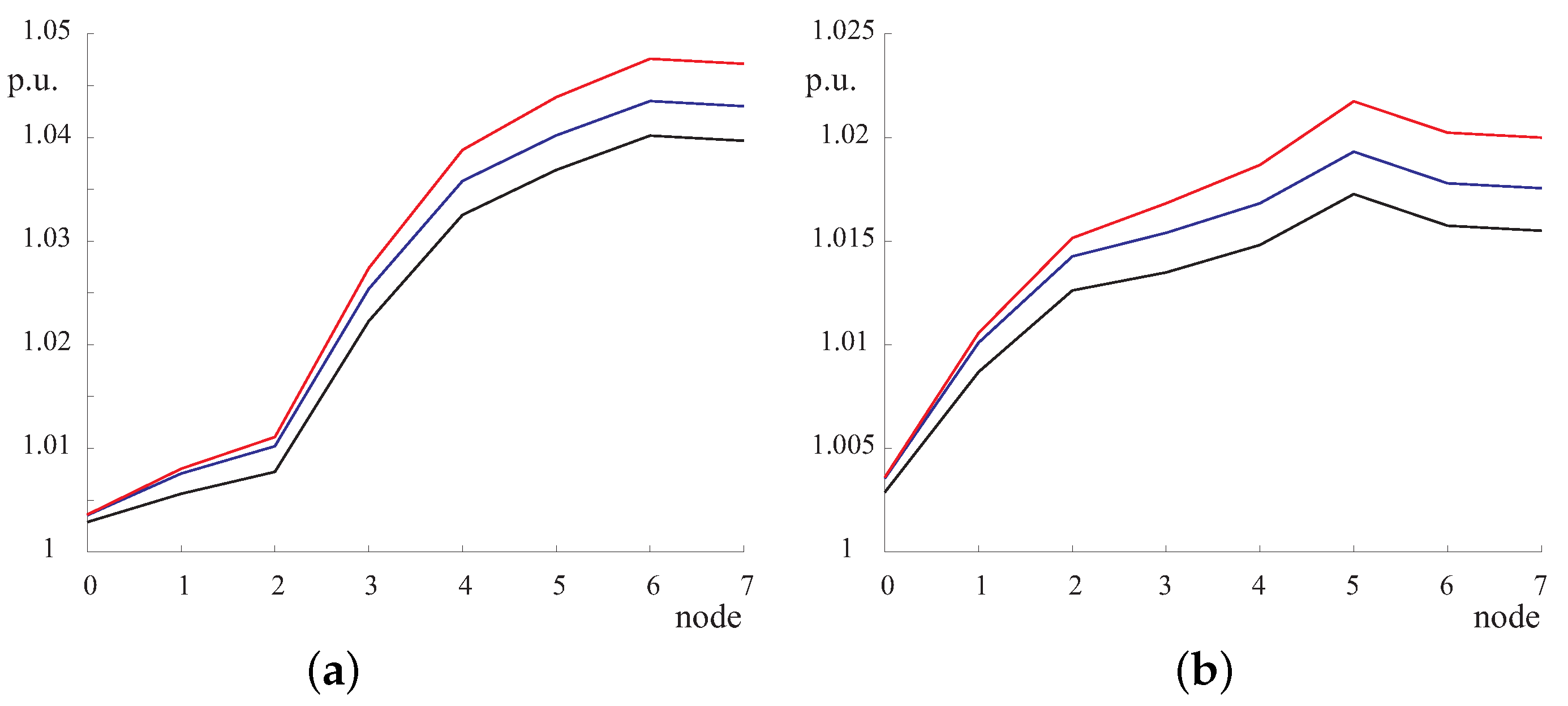
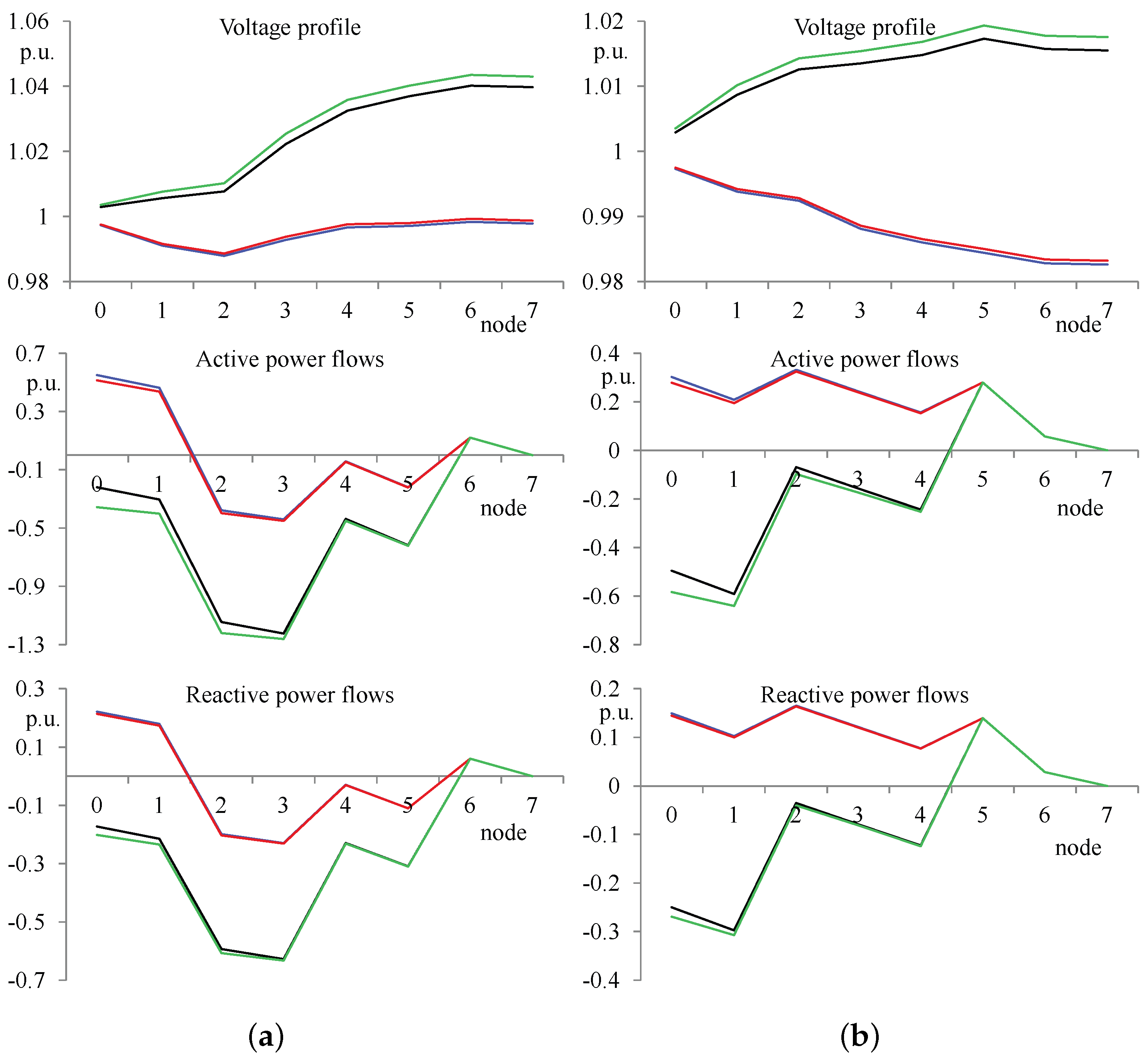
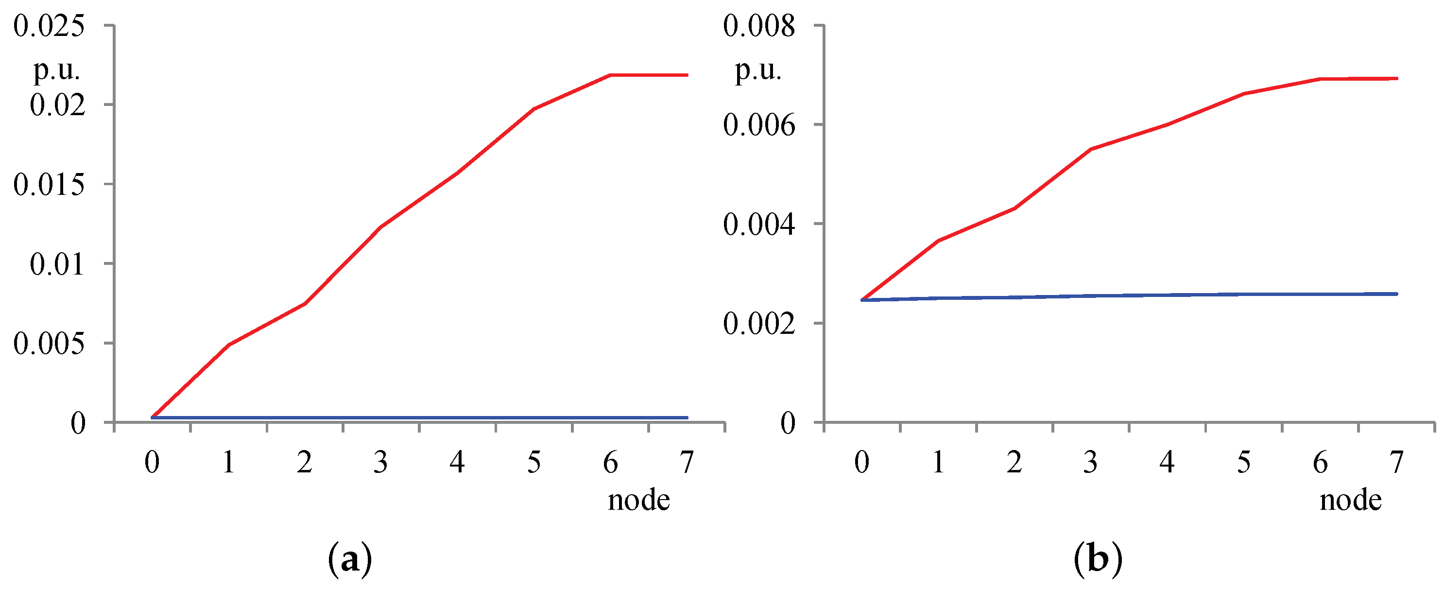
3.2. Model Validation

Starting from the initial operating condition in which all the power injections by the DERs are null, the proposed method is applied and the sensitivity matrices U j , k h and T j , k h , i in Equation (25) are evaluated. Then, new operating conditions are considered, characterized by active P D E R and reactive Q D E R power injections by the DERs. In particular, two different conditions are considered:
  • Case A: P D E R , g = 10 kW and Q D E R , g = 5 kVAr for g = 1 , , 4 ,
  • Case B: P D E R , g = 20 kW and Q D E R , g = 10 kVAr for g = 1 , , 4 .
In both of the cases, the variations of nodal voltages and active and reactive power flows along the two feeders are evaluated by Equation (25) and added to the corresponding initial values, yielding the final values. These latter ones are compared with the results obtained by solving the load flow using MATPOWER in both Cases A and B. The results are compared in Figure 6 for feeder 1 (a) and 2 (b). In each figure, the first graph reports the nodal voltage amplitudes, and the second and the third graphs, respectively, the branch active and reactive power flows along the considered feeder. In each graph, the results obtained by the proposed method and by the load-flow solution are plotted for Cases A and B.
Considering feeder 1 (Figure 6a), in Case A, the evaluated voltage profile presents a decreasing trend from the substation LV busbar until node 2, and, then, it inverts its trend until node 6, in which, again, the voltage presents a slight decrease towards the end of the feeder. The reason for such a voltage profile is to be found in the power flows reported in the other graphs, which present two inversions, one between nodes 1 and 2, and the other one between nodes 5 and 6. In Case B, the voltage profile is strictly increasing along feeder 1 except for the last branch, because of the negative values of active and reactive powers, that is power flows toward the supplying substation. It is worth noting that the powers flowing out at the last nodes of the feeders are always null because the proposed model imposes the border constraints (8). In both of the cases and in all of the graphs, it is apparent that the results obtained by the proposed method accurately follow the same trend as the ones obtained by the load-flow solution. Similar considerations can be made analyzing feeder 2 (Figure 6b). Since loading conditions and DER allocations differ with respect to feeder 1, different voltage profiles and power flows are obtained. In Case A, power flows always remain positive, and, consequently, the voltage profile is strictly decreasing along the feeder. In Case B, power flows are negative from the LV substation until node 4 and then positive from node 5 until the end of the feeder; consequently, the voltage profile is increasing until node 5 and then slightly decreasing. In addition, for this feeder, the results obtained by the proposed method present the same trends as the ones obtained by load-flow solution.
To quantify the accuracy of the results with respect to the ones obtained by load-flow solution, the maximum relative errors on the variations of the nodal voltage amplitudes and on the branch active and reactive power flows along each feeder are reported in Table 2 for Cases A and B. The relative errors are always limited to between 1 and 9 %. The largest errors are obtained in Case B and feeder 1, which actually represents an extreme operating condition as clearly evidenced by the voltage profile in Figure 6.

3.3. Comparison with a Perturb-and-Observe Method

The proposed method is compared with an alternative method that is used for sensitivity analysis, namely a perturb-and-observe method of the type in [15]. In this approach, the values of the system variables in an assigned initial operating condition of the distribution system are evaluated by solving a load flow. Then, a small DER injection, firstly of active power and secondly of reactive power, for one node at a time, is added to the initial operating condition and a new load-flow is solved. Finally, the sensitivity coefficients of the system variables with respect to each DER injection are evaluated as the ratio between the variations of the system variables with respect to their corresponding values in the initial operating condition and the amplitude of the considered DER injection. In particular, for the considered distribution system, the same initial operating condition as the one adopted for the proposed method is assumed, in which all the power injections by the DERs are null. Then, small injections of active power (1 kW) and of reactive power ( 1 kVAr) are imposed on one node at a time, for all the 14 nodes along the feeders: the variations of the system variables and the related sensitivity coefficients are obtained by 28 load-flow solutions.
Comparing the proposed method with the perturb-and-observe one in terms of computation times of the sensitivity coefficients, both methods require the solution of a load-flow in the same initial operating condition. The computation time of this load-flow solution is assumed as reference time unit and indicated as LF. The proposed method evaluates the coefficient matrices in Equation (25) using the closed-form expressions derived in Section 2 and the related computation time is equal to 0.20 LF. On the other hand, the perturb-and-observe method evaluates the sensitivity coefficients by 28 load-flow solutions with a computational time equal to 17.6 LF (it is less than 28 LF because of computational efficiency improvements that can be introduced). In conclusion, even for a small network as the considered one, the proposed method requires a computational time smaller of two orders of magnitude than the one required by a perturb-and-observe method.
To compare the proposed method with the perturb-and-observe one in terms of accuracy of the results, Case B defined in Section 3.2 is considered. Firstly, the voltage variations due to the DER injections are evaluated by using, respectively, the sensitivity coefficients for the perturb-and-observe method and Equation (25) for the proposed method. Then, the voltage variations are added to the corresponding values of the nodal voltages in the initial operating condition, yielding the new voltage amplitudes that account for the DER injections. In Figure 7, such voltage amplitudes evaluated by the proposed method, and by the perturb-and-observe method, are reported for both feeders and compared with the exact values provided by a load-flow solution in Case B. From the comparison, it is apparent that the results provided by the proposed method are more accurate than the ones obtained by the perturb-and-observe method. The main reason is that the proposed method uses the analytical derivative functions rather than the numerical derivatives used by the perturb-and-observe method.

3.4. Distributed Energy Resources Impact Evaluation

In the following, an example of the application of the proposed method to the evaluation of the impact of DERs on the nodal voltages of the distribution system is described to give evidence of the effectiveness of the method. The injection by DER 2 connected to node 6 of feeder 1 and by DER 3 connected to node 2 of feeder 2 are considered. The advantage of the proposed method is its linearity that allows for separately analyzing the impact in terms of nodal voltage variations of active and reactive power injection by each DER, to separately analyze the impact of the injections P D E R 2 , Q D E R 2 , P D E R 3 , Q D E R 3 . Then, the impact of any combination of these injections can be obtained by simply adding the voltage variations that each considered injection produces at each node, provided that all voltage variation is referred to the same initial operating condition, which is always assumed to be the one in which all the power injections by DERs are null.
Referring to active power injection, Figure 8a reports the variations of the nodal voltage amplitudes along both feeders caused by imposing P D E R 2 = 10 kW and evaluated by the proposed method. The injection has a different impact on the two feeders. In particular, on feeder 1, to which DER 2 is connected, the power injection causes a significant variation of the nodal voltage profile, which increases starting from the LV busbar until node 6, and then remains quite constant until the end of the feeder. Concerning feeder 2, the power injection along the other feeder has a practically null effect on the nodal voltage profile. In conclusion, the active power injection has a large impact on the feeder to which the DER is connected; on the contrary, it has a negligible impact on other feeders because of its negligible impact on the voltage drop along the MV/LV transformer.
Referring to reactive power injection, Figure 8b reports the variations of the nodal voltage amplitudes along both feeders caused by imposing Q D E R 2 = 10 kVAr and evaluated by the proposed method. Concerning feeder 1, the reactive power injection causes a significant variation of the nodal voltage profile, which increases from the LV busbar until node 6, and then remains quite constant until the end of the feeder. Concerning feeder 2, there is a significant variation on all the nodal voltages, but the shape of the voltage profile does not change, since all the nodes are subject to approximately the same voltage variation. In conclusion, the reactive power injection has a significant impact on the feeder to which the DER is connected, but also on other feeders, because it causes a reduction of the voltage drop along the MV/LV transformer.
Comparing the graphs (a) and (b) in Figure 8, it is apparent that P D E R 2 has a higher impact on the nodal voltages of feeder 1 with respect to Q D E R 2 because the branch resistances R j are larger than the branch reactances X j (Table 1); on the contrary, Q D E R 2 has a higher impact on the nodal voltages of feeder 2 with respect to P D E R 2 because the substation reactance X e q is larger than the substation resistance R t r .
Similar considerations can be made for Figure 9, which reports the voltage variations caused by imposing P D E R 3 = 10 kW (a) and Q D E R 3 = 10 kVAr (b). In this case, the major impact is on the voltages of feeder 2, where DER 3 is connected.
Comparing Figure 8 and Figure 9, it is apparent that the impact on the voltage profile of DER 2 on feeder 1 is higher than the impact of DER 3 on feeder 2 because the former DER 2 is connected near the end of feeder 1, whereas the latter DER 3 is connected near the beginning of feeder 2. On the contrary, the impacts of DER 2 on feeder 2 and of DER 3 on feeder 1 are very similar, which is negligible for active power injections and about 0 . 0024 p.u. for reactive power injections. Then, the impact of a DER on the voltage profile of a feeder, other than the one at which the DER itself is connected, does not depend on the position of the connection node.
Using the voltage variations that quantify the impact of each DER injection, it is possible to:
  • Identify the VMs with respect to voltage regulation problems: e.g., from the graphs (a) in Figure 8 and Figure 9, it is apparent that the two feeders belong to two different VMs as far as active power injections are considered;
  • Quantify the effectiveness of each DER on the voltage regulation in a VM: e.g., from the comparison of Figure 8 and Figure 9, it is apparent that DER 2 has a major effect on the voltage regulation of a VM along feeder 1 with respect to DER 3 ;
  • Quantify the interaction between the voltage regulation devices that are installed in a VM [17]: e.g., if a VM is defined along feeder 1, the voltage variation at node 4 caused by DER 2 and the voltage variation at node 6 caused by DER 1 represent the interaction between the voltage regulators acting on DER 1 and DER 2 .

4. Conclusions

A new model of LV distribution systems with DERs has been proposed, which is suitable for aggregating an existing distribution system into a cluster of virtual microgrids. The model is based on a linearized formulation of the branch flow equations and of the MV/LV supplying system. Then, the model is solved by imposing the border constraints at the MV busbar of the substation and at the end-nodes of the feeders and the coupling equations at LV substation busbar. The resulting closed form solution expresses the variations of the electrical variables of the LV distribution network as linear functions of the DERs injections. A numerical case study has evidenced the satisfactory accuracy of the results obtained by the proposed method with respect to the exact load flow solution. A comparison of the proposed method with a perturb-and-observe method is discussed with reference to computation time and accuracy of the results, thus giving evidence of the better performance of the proposed method. Eventually, an application to the evaluation of the impact of DERs on the voltage regulation problem of an LV distribution system has been presented, quantifying the sensitivity of the nodal voltages to the active and reactive power injections. Future work will extend the model to account for more complex network topologies and for unbalanced operating condition.

Author Contributions

The main contributions to the introduction and to the model development were brought by Anna Rita Di Fazio and Sara Valeri. The model application was performed by Michele De Santis. The case study was developed by Sara Valeri and Michele De Santis. The coordination of the work was up to Mario Russo. All the authors equally contributed to the paper writing.

Conflicts of Interest

The authors declare no conflict of interest.

References

  1. Bouhafs, F.; Mackay, M.; Merabti, M. Links to the future: Communication requirements and challenges in the smart grid. IEEE Power Energy Mag. 2013, 58, 2818–2833. [Google Scholar] [CrossRef]
  2. Belhomme, R.; Cerero Real De Asua, R.; Valtorta, G.; Paice, A.; Bouffard, F.; Rooth, R.; Losi, A. ADDRESS—Active demand for the smart grids of the future. In Proceedings of the CIRED Seminar: SmartGrids for Distribution, Frankfurt, Germany, 23–24 June 2008.
  3. Casolino, G.M.; Losi, A. Load areas in distribution systems. In Proceedings of the 15th IEEE International Conference on Environment and Electrical Engineering (EEEIC 2015), Rome, Italy, 10–13 June 2015.
  4. Di Fazio, A.R.; Erseghe, T.; Ghiani, E.; Murroni, M.; Siano, P.; Silvestro, F. Integration of renewable energy sources, energy storage systems, and electrical vehicles with smart power distribution networks. J. Ambient Intell. Humaniz. Comput. 2013, 4, 663–671. [Google Scholar] [CrossRef]
  5. Vandoorn, T.L.; Zwaenepoel, B.; Kooning, J.D.M.D.; Meersman, B.; Vandevelde, L. Smart microgrids and virtual power plants in a hierarchical control structure. In Proceedings of the 2011 2nd IEEE PES International Conference and Exhibition on Innovative Smart Grid Technologies (ISGT Europe), Manchester, UK, 5–7 December 2011.
  6. Arefifar, S.A.; Mohamed, Y.; El-Fouly, T. Optimized multiple microgrid-based clustering of active distribution systems considering communication and control requirements. IEEE Trans. Ind. Electr. 2015, 62, 711–723. [Google Scholar] [CrossRef]
  7. Di Fazio, A.R.; Fusco, G.; Russo, M. Decentralised voltage regulation in smart grids using reactive power from renewable DG. In Proceedings of the 2012 IEEE International Energy Conference and Exhibition (ENERGYCON 2012), Florence, Italy, 9–12 September 2012.
  8. Huang, J.; Jiang, C.; Xu, R. A review on distributed energy resources and MicroGrid. Renew. Sustain. Energy Rev. 2008, 12, 2472–2483. [Google Scholar]
  9. Brenna, M.; Berardinis, E.D.; Carpini, L.D.; Foiadelli, F.; Paulon, P.; Petroni, P.; Sapienza, G.; Scrosati, G.; Zaninelli, D. Optimal distributed voltage regulation for secondary networks with DGs. IEEE Trans. Smart Grid 2013, 4, 877–885. [Google Scholar] [CrossRef]
  10. Kumar, V.; Gupta, I.; Gupta, H.; Agarwal, C. Voltage and current sensitivities of radial distribution network: A new approach. IEE Proc. Gener. Transm. Distrib. 2005, 152, 813–818. [Google Scholar] [CrossRef]
  11. Khatod, D.K.; Pant, V.; Sharma, J. A novel approach for sensitivity calculations in the radial distribution system. IEEE Trans. Power Deliv. 2006, 21, 2048–2057. [Google Scholar] [CrossRef]
  12. Zhou, Q.; Bialek, J.W. Simplified calculation of voltage and losses sensitivity factors in distribution networks. In Proceedings of the 16th Power Systems Computation Conference (PSCC2008), Glasgow, Scotland, UK, 14–18 July 2008.
  13. Weckx, S.; D’Hulst, R.; Driesen, J. Voltage sensitivity analysis of a laboratory distribution grid with incomplete Data. IEEE Trans. Smart Grid 2015, 6, 1271–1280. [Google Scholar] [CrossRef]
  14. Gurram, R.; Subramanyyam, B. Sensitivity analysis of radial distribution network—Adjoint network method. Int. J. Electr. Power Energy Syst. 1999, 21, 323–326. [Google Scholar] [CrossRef]
  15. Tamp, F.; Ciufo, P. A Sensitivity analysis toolkit for the simplification of MV distribution network voltage management. IEEE Trans. Smart Grid 2014, 5, 559–568. [Google Scholar] [CrossRef]
  16. Di Fazio, A.R.; Russo, M.; Valeri, S.; De Santis, M. LV distribution system modeling for distributed energy resources. In Proceedings of the 2016 16th IEEE International Conference on Environment and Electrical Engineering (EEEIC 2016), Florence, Italy, 7–10 June 2016.
  17. Di Fazio, A.R.; Fusco, G.; Russo, M. Decentralized voltage control of distributed generation using a distribution system structural MIMO model. Control Eng. Pract. 2016, 47, 81–90. [Google Scholar] [CrossRef]
  18. Baran, M.; Wu, F. Optimal sizing of capacitors placed on a radial distribution system. IEEE Trans. Power Deliv. 1989, 4, 735–743. [Google Scholar] [CrossRef]
  19. Zimmerman, R.D.; Murillo-Sánchez, C.E.; Thomas, R.J. MATPOWER: Steady-state operations, planning and analysis tools for power systems research and education. IEEE Trans. Power Syst. 2011, 26, 1–19. [Google Scholar] [CrossRef]
Figure 1. Low Voltage distribution system with Distributed Energy Resources.
Energies 09 00801 g001
Figure 2. Electric equivalent circuit of the Medium/Low Voltage substation.
Energies 09 00801 g002
Figure 3. Electric equivalent circuit of the j-th branch of a feeder.
Energies 09 00801 g003
Figure 4. Electric equivalent circuit of the h-th feeder.
Energies 09 00801 g004
Figure 5. Case study distribution system.
Energies 09 00801 g005
Figure 6. Voltage amplitudes and power flows along feeder 1 (a) and feeder 2 (b) evaluated by the proposed model and by load flow solution: Case A—proposed model (red) and load-flow (blue); Case B—proposed model (green) and load-flow (black).
Energies 09 00801 g006
Figure 7. Voltage amplitudes in the case B for feeder 1 (a) and feeder 2 (b) evaluated by the exact load-flow (black); the proposed method (blue) and the perturb-and-observe method (red).
Energies 09 00801 g007
Figure 8. Voltage variations in the case of P D E R 2 = 10 kW (a) and of Q D E R 2 = 10 kVAr (b) for feeder 1 (red) and feeder 2 (blue).
Energies 09 00801 g008
Figure 9. Voltage variations in the case of P D E R 3 = 10 kW (a) and of Q D E R 3 = 10 kVAr (b) for feeder 1 (red) and feeder 2 (blue).
Energies 09 00801 g009
Table 1. Electrical parameters and loads for the branches of both the feeders. p.u.: per unit.
From NodeTo NodeBoth FeedersFeeder 1Feeder 2
R (p.u.)X (p.u.)PL (p.u.)QL (p.u.)PL (p.u.)QL (p.u.)
010.01050.00250.08320.04160.09280.0464
120.00600.00140.84000.37800.27560.1376
230.01140.00270.06000.03000.08720.0436
340.00800.00110.00.00.08720.0436
450.00950.00140.17760.08000.27560.1376
560.00520.00070.06000.03000.22200.1112
670.00400.00060.12000.06000.05720.0284
Table 2. Maximum relative errors.
CaseFeeder NumberMaximum Errors (%) on the Variations of
Voltage AmplitudesActive Power FlowsReactive Power Flows
A13.34.41.9
23.12.81.3
B16.58.53.6
25.55.42.4

