Article

Neural Network Ensemble Based Approach for 2D-Interval Prediction of Solar Photovoltaic Power

1
Centre for Translational Data Science, University of Sydney, Sydney, NSW 2006, Australia
2
School of Information Technologies, University of Sydney, Sydney, NSW 2006, Australia
*
Author to whom correspondence should be addressed.
Energies 2016, 9(10), 829; https://doi.org/10.3390/en9100829
Submission received: 31 July 2016 / Revised: 28 September 2016 / Accepted: 30 September 2016 / Published: 17 October 2016
(This article belongs to the Special Issue Energy Time Series Forecasting)

Abstract

:
Solar energy generated from PhotoVoltaic (PV) systems is one of the most promising types of renewable energy. However, it is highly variable as it depends on the solar irradiance and other meteorological factors. This variability creates difficulties for the large-scale integration of PV power in the electricity grid and requires accurate forecasting of the electricity generated by PV systems. In this paper we consider 2D-interval forecasts, where the goal is to predict summary statistics for the distribution of the PV power values in a future time interval. 2D-interval forecasts have been recently introduced, and they are more suitable than point forecasts for applications where the predicted variable has a high variability. We propose a method called NNE2D that combines variable selection based on mutual information and an ensemble of neural networks, to compute 2D-interval forecasts, where the two interval boundaries are expressed in terms of percentiles. NNE2D was evaluated for univariate prediction of Australian solar PV power data for two years. The results show that it is a promising method, outperforming persistence baselines and other methods used for comparison in terms of accuracy and coverage probability.

1. Introduction

Generating electricity from renewable sources is a key factor in the transition to a clean and sustainable energy future, to address environmental concerns and limit the global warming. Solar energy generated from PV systems is one of the most promising and fastest growing types of renewable energy [1]. This growth is driven by government incentives that encourage the use of solar energy and by the decreasing cost of PV panels, making them more affordable. Since 2000, the installation of PV systems worldwide has increased 100 times, reaching 178 GW in 2014, and this capacity is expected to triple by 2019 [2]. It is also expected that by 2050 PV systems will provide 29% of the electricity in Australia [3] and 25% of the electricity in Europe [4].
In comparison to the traditional fossil and nuclear energy sources, solar energy is freely available, can be easily harnessed and is environmentally free. However, unlike the traditional energy sources, it is highly variable as it depends on the solar irradiance, cloud cover and other meteorological factors. This creates challenges for its mass integration in the electricity grid. The European Photovoltaic Industry Association has identified forecasting as one of the key factors enabling large-scale integration of solar power in the electricity grid [4]. Accurate forecasting ensures reliable supply, reduces the costs by allowing more efficient and secure management of electricity grids and also supports solar energy trading at electricity markets [4].
Solar power forecasting has been an active area of research. A comprehensive review of the state-of-the-art methods for PV power forecasting is presented in [5]. There are two groups of forecasting approaches: indirect and direct. The indirect approaches firstly forecast the solar irradiance or use forecasts of solar irradiance produced by meteorological centers, and then convert them to PV power forecasts by considering the characteristics of the PV plant. The second group directly forecasts the PV power output. Notable examples of the first group are [6,7,8,9,10]. For example, Lorenz et al. [6] predicted the hourly PV power output for up to 2 days ahead based on the weather forecasts of solar irradiance. They also derived regional power forecasts by up-scaling the forecasts of representative PV systems. Urraca et al. [10] predicted the solar irradiance 1 h ahead based on recorded meteorological data and computed solar variables. They developed two types of models: fixed and moving, and applied a number of prediction algorithms—Support Vector Regression (SVR), random forests, linear regression and nearest neighbor.
Recent examples of the second group, direct forecasting approaches, include [11,12,13,14,15,16,17]. For example, Chen et al. [12] predicted the PV power output for the 24 h of the next day using the PV power from the previous day and the weather forecast for the next day. They classified the days into sunny, cloudy and rainy, and built a separate prediction model, a Radial-Basis Function Neural Network (RBFNN), for each category. A Self-Organising Map (SOM) was used to learn the characteristics of the three types of days based on the weather predictions of solar irradiance and cloudiness. To forecast the PV output for a new day, SOM was firstly used to output the type of the day, and then the RBFNN model for this type of day was used to generate the prediction. Pedro and Coimbra [11] predicting the PV power 1 and 2 h ahead from previous PV power data by using Autoregressive Integrated Moving Average (ARIMA), nearest neighbors and Neural Networks (NNs) methods.
While the focus in previous work has been on point forecasting, in this paper we consider interval forecasting, and in particular 2D-interval forecasting, which was recently introduced by Torgo and Ohashi [18]. The differences between the three types of forecasting tasks–point, interval and 2D-interval can be summarized as follows: (1) Point forecasts predict a single value—at time t the task is to predict the value of the time series for time t + h, where h is the forecasting horizon (h = 1 for 1-step ahead prediction); (2) Interval forecasts predict an interval of plausible values. A standard interval forecast consists of an upper and lower bound, between which a single future value is expected to lie with high probability [19], i.e., at time t the task is to predict an interval of plausible values of the time series for time t + h; (3) A 2D-interval forecast [18] is an interval forecast for a range (or an interval) of future values not a single value, i.e., at time t the task is to predict the upper and lower bound for the range of future values [t + h, t + k].
Although point forecasts are the most common types of forecasts, interval forecasts are more useful than point forecasts for applications requiring risk management and balancing of demand and supply, such as electricity production, electricity and financial markets, water distribution and manufacturing [18,19]. Predicting an interval of plausible values instead of only predicting a single value gives more information about the variability of the target variable, which in turn can help to assess the uncertainty of the future values and be used to make more accurate decisions. 2D-interval forecasts are particularly relevant for applications where the predicted variable has a high inherent variability, such as solar and wind power prediction.
Torgo and Ohashi [18] showed an application of 2D-interval forecasting for two water prediction tasks: predicting the values of water quality parameters (e.g., pH, iron, etc.) in a distribution network for a metropolitan area in Portugal and predicting the water consumption in a residential area network in Spain. In our previous work [20] we presented an application of 2D-interval forecasting for solar power prediction from previous PV power and weather data. We predicted the maximum and minimum values of the interval, using a SVR based method. In this paper we extend our previous work by predicting summary statistics (10–90th and 25–75th percentiles) instead of the maximum and minimum values, applying feature selection using Mutual Information (MI) and using an ensemble of NNs as a classification algorithm. In this work we also use only previous PV power data instead of both PV power and weather data, and show that it is sufficient for good prediction.
The contribution of our work is the following:
(1)
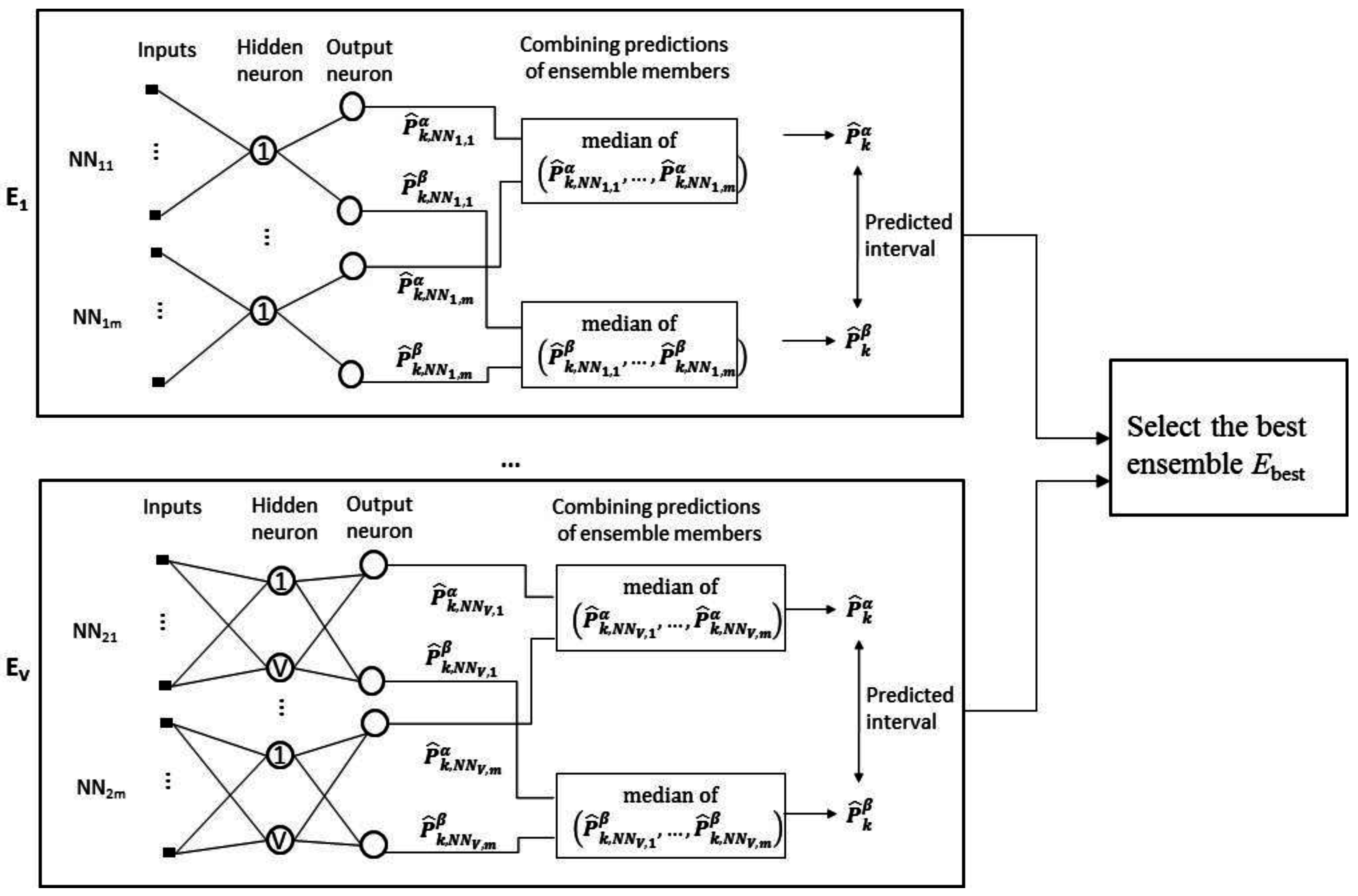
We consider the task of interval forecasting for solar power generated by PV systems. Specifically, we consider 2D-interval forecasting where we predict two summary statistics for a future interval of PV power values—10–90th and 25–75th percentiles. Our proposed approach called Neural Network Ensemble for 2D-interval forecasting (NNE2D) uses MI to select a small set of informative variables and an ensemble of NNs for prediction. It doesn’t require any previous weather data or future weather predictions; it only uses previous PV power data.
(2)
We evaluate the performance of NNE2D using Australian data for two years, sampled at 5-min intervals, for three different interval lengths (from 1 h to 3 h). We compare the results with two persistence methods used as baselines, a model based on SVR and also with our two multivariate approaches from [20]. The results show that NNE2D is a promising approach, outperforming the other methods in terms of accuracy and coverage probability, and hence is a viable method for practical applications.
This paper is organized as follows. Section 2 describes the data used in this study and Section 3 provides a problem statement. Section 4 describes our proposed approach NNE2D for computing 2D-interval forecasts and Section 5 presents the methods used for comparison. Section 6 describes the experimental setup. Section 7 presents and discusses the results, and Section 8 concludes the paper.

2. Data

We use solar power data from the largest flat-panel, grid-connected, PV system in Australia. It is located at the St Lucia campus of the University of Queensland in Brisbane and has about 5000 solar panels distributed at the roof-top of four buildings, generating up to 1.22 MW of electricity.
The data is measured at 1-min intervals for 24 h. We collected data for 10 h during the day, from 7:00 am to 5:00 pm, for two complete years—from 1 January 2013 to 31 December 2014. Outside these 10 h the solar power is either zero or very low due to the absence of solar irradiation. The data is publicly available at [21].
The original data set consists of 2 × 365 × 600 = 438,000 measurements in 1-min resolution. There were only 1518 missing values which is about 0.35%. Each missing value was replaced by the average of the values from the previous 5 min, i.e., with the 5 most recent observations of the PV power output. The 1-min data was aggregated into 5-min intervals by averaging every 5 consecutive measurements, resulting in 2 × 365 × 120 = 87,600 measurements in total. The data was normalized to the range (0,1).
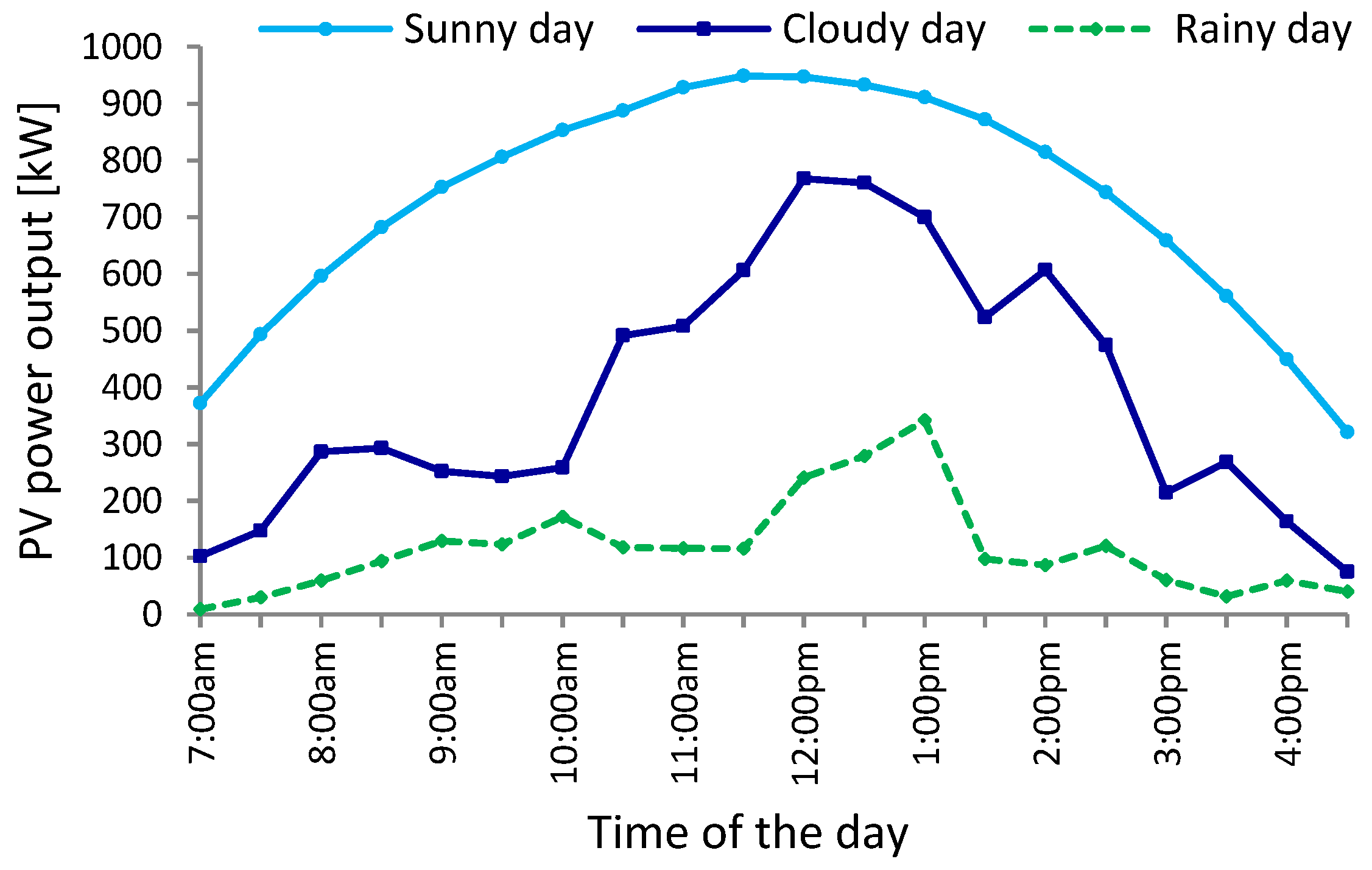
The generated PV power depends on the weather conditions, especially the solar irradiance. Figure 1 plots the solar power profiles at half-hourly intervals, for three different types of days: sunny (13 April 2013), cloudy (15 April 2013) and rainy (20 April 2013). The three graphs differ considerably—for sunny days, the power output from a PV system is the highest and typically follows a bell shaped curve; for cloudy and rainy days, the generated PV power is lower and it varies during the day due to the changes in the weather conditions.

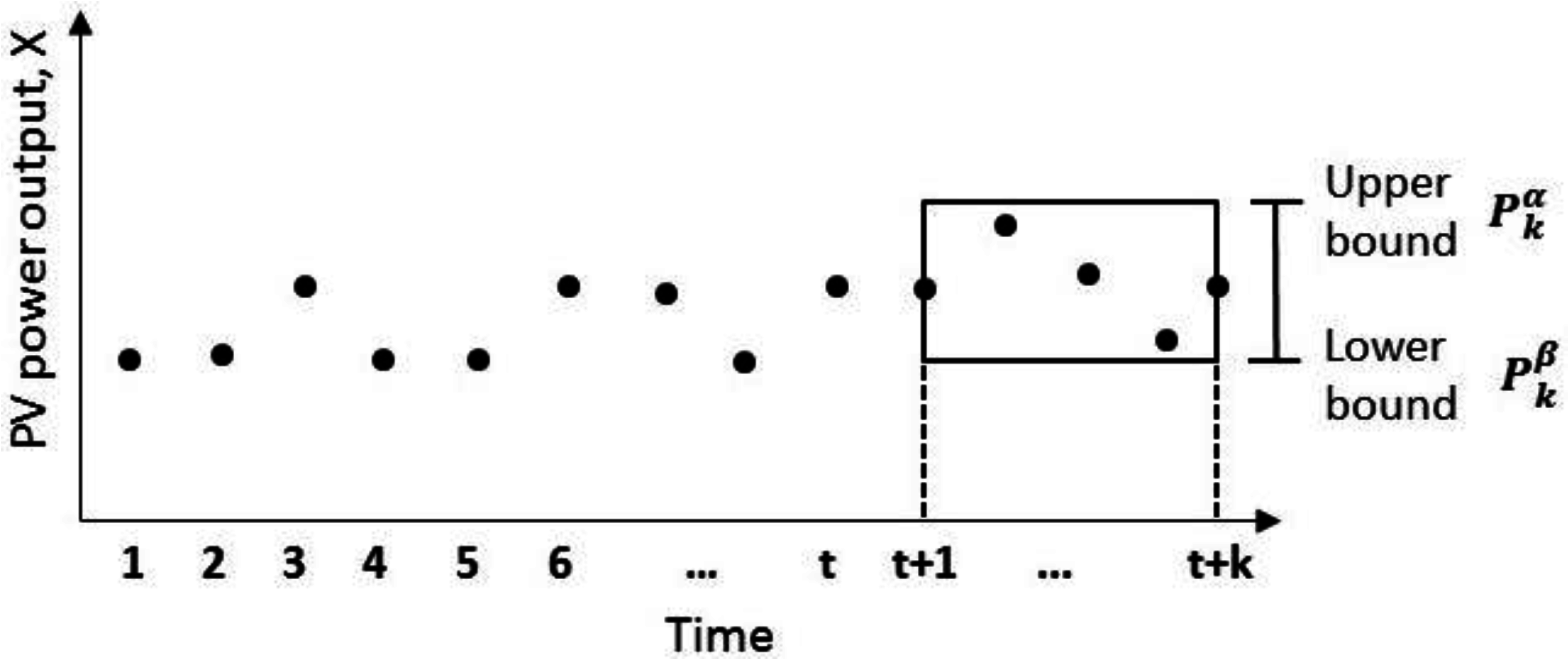
3. Problem Definition

Let X = X 1 ,   X 2 ,   ,   X t be a discrete time series of PV power outputs up to time t . Our goal is to compute the 2D-interval forecast for the next interval with length k, i.e., for the values X t + 1 ,   X t + 2 ,   ,   X t + k . Specifically, at time t we predict the upper and lower bounds for the values of X in the interval [ t + 1 ,   t + k ] (see Figure 2).
There are different ways to construct the upper and lower bounds of the k -length interval using descriptive statistics—e.g., using the 75th and 25th percentiles as in [18] or using the maximum and minimum values as in [20]. In this study, we follow the first method as percentiles are more robust to noise and outliers than minimum and maximum values. Let P k α and P k β are the α and β percentiles ( α > β ) for the PV power time series X for the k -length future time interval [ t + 1 ,   t + k ] . The interval formed by them corresponds to the interval where | α β | × 100 % of the values of X are expected to lie [6]. In this work, we construct two types of 2D-interval forecasts: by using the 90th and 10th percentiles, as well as 75th and 25th percentiles. However, our method is general and can be used for intervals with different bounds and lengths, depending on the specific application and scenario.

4. Proposed Approach NNE2D

Figure 3 presents a block diagram of NNE2D. It uses an ensemble of NNs for computing the 2D-interval forecasts and includes three main steps: (1) variable selection; (2) training and selection of the NN ensemble; and (3) forecasting of new data, as described below.

4.1. Variable Selection

Variable (or feature) selection is a key factor affecting the performance of prediction systems [22,23]. The goal is to select a set of input variables that are relevant, important and sufficient for predicting the target variable.
To select lag variables, we used a method based on MI. MI is an information theoretic measure of the relationship between two variables X and Y —it measures the amount of information obtained from X in the presence of Y and vice-versa. If the two variables are independent, MI is zero; if they are dependent, MI has a positive value corresponding to the strength of the relationship. In contrast to traditional feature selection methods for time series such as autocorrelation which capture only linear dependencies, MI is able to detect both linear and non-linear dependencies. To compute MI we applied the method of Kraskov et al. [24] which is based on nearest neighbor distances.
We extract all lag variables from a time window with length one day (120 lag variables in total) and calculate the MI score between each of them and the targets P k α and P k β , for intervals with different lengths: k = 12, 24 and 36. One day of previous data is sufficient as the PV power is affected by changes in the solar irradiance and they are best captured in the most recent data. Figure 3 shows the MI score of the candidate lag variables for k = 12 and 24; the graph for k = 36 is similar and not shown. As we can see from Figure 4, the MI score drops sharply and then flattens. To select a set of predictive variables, we chose a cut-off threshold of MI = 0.6, which was satisfied by 5–6 variables for all three interval lengths. The cut-off threshold was chosen empirically; our goal was to select a small set of highly predictive variables. Further analysis revealed that the selected variables were variables extracted from the previous 30 min, which shows the importance of the most recent data. We chose the previous 6 PV lag variables for inclusion in the final feature set and validated this selection by increasing the number of variables up to 12, one at a time, but found that the inclusion of variables beyond lag 6 does not improve the prediction accuracy.
In addition to the 6 selected lag variables, following [20] we also selected the upper and lower bounds, P k 1 α and P k 1 β , of the previous k -length interval X t k + 1 , , X t 1 ,   X t . These features provide useful information about the recent dynamics of the two percentiles that we are trying to predict. Thus, we use 8 features in total as listed in Table 1.

4.2. Prediction Model—NN Ensemble

As a prediction model for P k α and P k β , we use an ensemble of NNs. NNs are one of the most popular prediction algorithms for solar power forecasting [11,14,25], and also for other energy time series such as electricity load forecasting [26,27,28]. However, their performance is very sensitive to the NN architecture and the random initialization of weights. By combining the predictions of several NNs in an ensemble, this sensitivity can be reduced. Ensembles of prediction algorithms are also typically more accurate than a single ensemble member [29].
We adapt our NN ensemble method from [30] which was previously applied for point forecasting; we call the adapted prediction model NNE2D.
Single NN. A single NN, part of NN2D, is a multilayer perceptron NN as shown in Figure 5. It has p input neurons corresponding to the selected features, two output neurons for P k α and P k β and one hidden layer where the number of hidden neurons is determined experimentally as described below. The NN weights are initialised to random values using the Nguen-Widrow method [31].
Each single NN is trained separately on the training data using the Levenberg Marquardt (LM) algorithm [32] to minimize the mean squared error on the training data. LM has been chosen over the standard steepest gradient descent backpropagation algorithm because of its faster convergence.
The training is terminated when one of the following conditions is met: (1) the maximum number of training epochs (1000) is reached; (2) no improvement in the performance on the validation set is observed for a certain number of epochs (10); or (3) the performance gradient becomes very small (less than 1 × 10⁻⁷).
Ensemble of NNs. We build V ensembles of NNs and then select the best one, as shown in Figure 6. Each ensemble combines the predictions of m NNs with the same number of hidden neurons but different initialization of the weights. For example, the ensemble E V combines the predictions of m NNs with V hidden neurons. The combination is done by taking the median of all m predictions. In our experiments we used m = 10 and V = 30.
After each NN is trained separately on the training data, the performance of the V ensembles is evaluated on the validation set and the best performing ensemble E b e s t , the one with the lowest prediction error (MRE) on the validation set, is selected and used to predict the testing data.

4.3. Predicting New Data

To predict P k α and P k β for a new example i, the ensemble E b e s t combines the predictions of its ensemble members (i.e., single NNs) by taking the median of their predicted lower and upper bounds as shown in Figure 6. This means that: P ^ k α = m e d i a n ( P ^ k ,   N N b e s t , 1 α , , P ^ k ,   N N b e s t , m α ) and P ^ k β = m e d i a n ( P ^ k ,   N N b e s t , 1 β , , P ^ k ,   N N b e s t , m β ) , where P ^ k ,   N N b e s t , j α and P ^ k ,   N N b e s t , j β are the predictions for the α and β percentiles generated by an N N j of ensemble E b e s t , j = 1 ,   ,   m .

5. Methods Used for Comparison

To provide a comprehensive evaluation of NNE2D, we compare its performance with two persistence models and a method similar to NNE2D but using SVR instead of an NN ensemble.

5.1. Persistence Models

We use two persistence models as baselines for comparison. Persistence models consider the recently observed values of time series data as predicted values and are used as baselines. We implemented two persistence models: B1 and B2.
The first baseline ( B 1 ) uses the previous k -length interval. The 2D-interval forecast at time t for the interval [t + 1, t + k] is given by the percentiles of the previous interval [tk − 1, t], i.e.,: P k 1 α = α percentile of ( P t k + 1 , ,   P t 1 ) and P k 1 β = β percentile of ( P t k + 1 , ,   P t 1 ) .
The second baseline ( B 2 ) uses the k-interval from the previous day, at the same time. The 2D-interval forecast at time t for the interval [t + 1, t + k] is given by using the percentiles of the time series for the interval [tkd + 1, td], where d is the total number of observations in a day, i.e., P k d α = α percentile of ( P t d k + 1 , ,   P t d ) and P k d β = β percentile of ( P t d k + 1 , ,   P t d ) . Zhang et al. [33] showed that for point forecasting a persistence model similar to B 2 was more accurate compared to ARIMA, NNs and SVR when the consecutives days have similar PV power characteristics.

5.2. SVR Based Method

We also evaluate the performance of SVR as a prediction algorithm instead of an NN ensemble, under the same experimental conditions. We call this method SVR2D.
SVR is an advanced prediction algorithm [34] that has shown excellent performance in several domains [35,36,37], including solar power forecasting, e.g., [9,13,38].
The key idea of SVR is to map the input data into a higher dimensional feature space using a non-linear transformation and then apply linear regression in the new space. The linear regression in the new space corresponds to nonlinear regression in the original space. The task is formulated as an optimisation problem. The main goal is to minimize the error on the training data, but the flatness of the line and the trade-off between training error and model complexity are also considered to prevent overfitting. The solution is defined by a small subset of training examples, called support vectors.
Solving the optimization problem requires computing dot products of input vector in the new space which is computationally expensive in high dimensional spaces. To help with this, kernel functions satisfying the Mercer’s theorem are used—they allow the dot products to be computed in the original lower dimensional space and then mapped to the new space.
Since SVR can have only one output, SVR2D divides the 2D-interval prediction task into two subtasks: predicting the upper bound P k α and predicting the lower bound P k β , and builds a separate SVR prediction model for each of them:
P k α = S V R ( X t 5 ,   X t 4 ,   X t 3 ,   X t 2 ,   X t 1 ,   X t , P k 1 α ,   P k 1 β )
P k β = S V R ( X t 5 ,   X t 4 ,   X t 3 ,   X t 2 ,   X t 1 ,   X t , P k 1 α ,   P k 1 β )
We used Radial Basis Function (RBF) kernel, which was selected after empirical evaluation and comparison of different kernel functions.

6. Experimental Setup

6.1. Training, Validation and Testing Sets

We divided the available solar power data for the two years (2013 and 2014) into three non-overlapping subsets: training (50%) validation (25%), and testing (25%). The data for 2013 was assigned to the training set, 50% of the data for 2014 was assigned to the validation set and the remaining 50% for 2014 was assigned to the testing set. Table 2 shows the number of samples in each subset.
The training set was used for feature selection and training of the prediction models, the validation set was used to tune the parameters of the prediction models, e.g., for selecting the best NN ensemble and kernel function for SVR2D. The testing set was used to evaluate the performance of the prediction models for 2D-interval forecasting.

6.2. Interval Length

We consider intervals with three different lengths: 1 h, 2 h and 3 h, and two different bounds: 90%–10% and 75%–25% percentiles. This allows us to better evaluate our approach under different conditions and also shows that it can be used in different scenarios by the power system operators depending on the task, e.g., real-time dispatching, storage management, etc. Table 3 summarizes the interval lengths in terms of steps k and time l, and also the bounds we used.

6.3. Evaluation Mesusres

We use three different evaluation measures: Mean Absolute Interval Deviation (MAID), Mean Relative Error (MRE) and Interval Coverage Probability (ICP):
M A I D = 1 2 N [ i = 1 n | P k , i α P ^ k , i α | + | P k , i β P ^ k , i β | ]
M R E = 1 2 N [ i = 1 n | P k , i α P ^ k , i α R | + | P k , i β P ^ k , i β R | ] · 100 %
I C P = 1 N × k i = 1 N j = i + 1 i + k c j · 100 %
where: P k , i α and P k , i β are the actual values of the upper and lower bounds of the k-length interval for i-th example in the dataset and P ^ k , i α and P ^ k , i β are the respective predicted values; k is the length of interval, N is the total number of examples in the dataset, R is the range of the target values of the PV power output data; and c j = {   1 ,       i f   X j [ P k , i α ,   P k , i β ]   0 ,       o t h e r w i s e                         .
MAID is standard measure for interval forecasts [18,20]. It measures the mean absolute deviation of the upper and lower bounds of the predicted intervals from the upper and lower bounds of the actual intervals. MRE measures the percentage deviation of the predicted intervals from the actual intervals normalized by the range of the target values. It is an extension of MAID and facilitates comparison of prediction errors for data sets with different range of values. Low values for both MAID and MRE indicate high prediction accuracy.
ICP measures the likelihood of the k values of the time series for the next k-length interval to be included in the predicted interval [ P ^ k α , P ^ k β ], averaged over all points in the data set. High coverage probability indicates high accuracy. For 2D-interval forecasts with upper and lower bounds constructed using α and β percentiles ( α > β ), the expected coverage probability is | α β | × 100 % .

7. Results and Discussion

7.1. Accuracy

Table 4 presents the accuracy results for NNE2D and Table 5 for the methods used for comparison. Figure 7 and Figure 8 show a visual comparison of the MRE and ICP results for all methods.
The results show that NNE2D outperformed the other methods for all interval lengths and interval boundaries, for all three evaluation measures. On average NNE2D achieved the following percentage improvements in terms of MAID and MRE: compared to SVR2D: 21.50%–24.40%, compared to B1: 44.65%–58.45% and compared to B2: 58.63%–61.66%. These improvements in terms of ICP are: 6.48%–21.04%, 83.7%–50.42% and 91.68%–75.58% respectively.
SVR2D is the second best method and it also considerably outperforms the two baselines. From the two baselines, B1 is more accurate than B2, which shows that the most recent solar data is more important than the data from the previous day for 2D-interval prediction. This is also supported by the performance of both NNE2D and SVR2D which utilise a small set of input variables from the most recent solar power data.
Figure 9 shows the regression results of the predicted and actual values for the upper and lower bounds of the 2D-intervals with lengths 1 h, α = 90th and β = 10th percentile. The regression plots for the remaining cases are very similar and not shown. We can see that most of the data falls along the diagonal line, with high values for the coefficient of determination R (0.88–0.90), indicating that the predicted and actual bounds of the 2D-intervals are very close to each other.

7.2. Performance for Different Interval Lenghts

From Table 4 we can see that the accuracy of NNE2D varies depending on the lengths of the intervals. The best accuracy results in terms of MAID and MRE are achieved for the intervals with the smallest length (l = 1 h, k = 12 steps). The accuracy decreases as the length of the predicted interval increases. These findings are as expected—it is generally easier to predict values that are closer in time to the current value.
In terms of coverage probability ICP, the results for the 10–90 percentile interval are similar for the different interval lengths while for the 25th–75th percentile interval ICP slightly increases with the increase of the interval length. We can also see that ICP is higher for the 10th–90th percentile interval than for the 25th–75th percentile interval. This is anticipated since the expected coverage probability drops from 80% (=90%–10%) for the first case to 50% (=75%–25%) for the second case.
To provide additional insights, Table 6 shows the Mean Interval Width (MIW) for the constructed intervals. Similarly to MAID and MRE, we can see that MIW increases as the interval length increases, and this holds for both predicted and actual intervals. MIW also depends on the upper and lower bounds of the intervals and as Figure 10 shows it is higher for the 10th–90th percentile interval than for the 25th–75th percentile interval. In summary, the analysis of ICP values from Table 4 and MIW values from Table 5 indicates that the coverage probabilities for wider intervals are higher. This is consistent with the results in [39] and as expected since the data points have a higher probability to fall in a wider interval, which implies a higher ICP.

7.3. Comparison with Previous Work

We also compare the performance of NNE2D with our previous work [20]. The two methods from [20] are based on SVR and a single NN (not an ensemble) and are denoted with SVR2D ref and NN2D ref . In contrast to NNE2D where we use only previous solar power data, S V R 2 D r e f and N N 2 D r e f use both meteorological and solar power data. In addition, SVR2D ref and NN2D ref predict the maximum and minimum values of the future interval, not percentile boundaries. For fair comparison, we evaluated the performance of NNE2D for predicting the same boundaries (maximum and minimum values).
Table 7 shows the comparison results. We can see that NNE2D is more accurate than SVR2D ref and NN2D ref . The average percentage improvement of NNE2D in terms of MAID or MRE is: 28.12% and 34.32% (compared to SVR2D ref and NN2D ref ) and this improvement in terms of ICP is 12.77% and 31.71%, respectively. This is a promising result, especially considering that it was achieved by using only previous power data, without any weather data. It also shows that for very-short term forecasting of up to 3 h ahead, there is no need to use weather data—the previous solar power data is sufficient.

7.4. Training of the NN Ensemble

To analyse the convergence behaviour of the individual NNs used in an NNE2D ensemble, we examine how the performance function (MSE) changes during the training phase. Figure 11 shows the convergence graph of MSE for a typical NN (an ensemble member). We can see that the initial MSE is high but as the training progresses it decreases rapidly. The training of the NN is terminated after 38 training epochs when the second stopping criterion is satisfied—the accuracy on the validation set does not improve for 10 consecutive epochs. In summary, the results show good and fast convergence.
The overall training time of NNE2D was 8–10 min (for a computer with Intel Core i7 3.4 GHz processing unit and 16 GB memory). This includes the time required to train all ensemble members and for combining their forecasts to generate the final prediction. The training time for a single NN varied from 50 s to 1 min. Convergence was typically achieved for 30–40 epochs, although the MSE was already very low after 5–10 epochs in most of the cases. The training time is a very important factor when the prediction models are used online, and particularly when they need to be re-trained often. Since the overall training time is only a few minutes, the proposed approach is suitable for both off-line and on-line training.

8. Conclusions

We considered the task of 2D-interval forecasting and its application for predicting the electricity power generated by solar PV systems. Specifically, at time t we predict summary statistics for the distribution of the PV power time series in the future time interval [t + 1, t + k] such as the 90th and 10th percentiles, and also the 75th and 25th percentiles. This type of forecasting task was recently introduced by Torgo and Ohashi in [18] and is useful to quantify uncertainty in applications which require balancing of demand and supply, especially when the predicted variable has a high variability such as in solar power forecasting.
Our proposed method NNE2D uses a variable selection based on MI and an ensemble of NNs to compute the lower and upper bounds (expressed as percentiles) of the 2D-interval forecasts. It was evaluated for predicting the solar PV power output using Australian PV power data for two years, sampled at 5-min intervals, for future intervals with length from 1 to 3 h. The prediction was done using only previous PV power data, without any weather data.
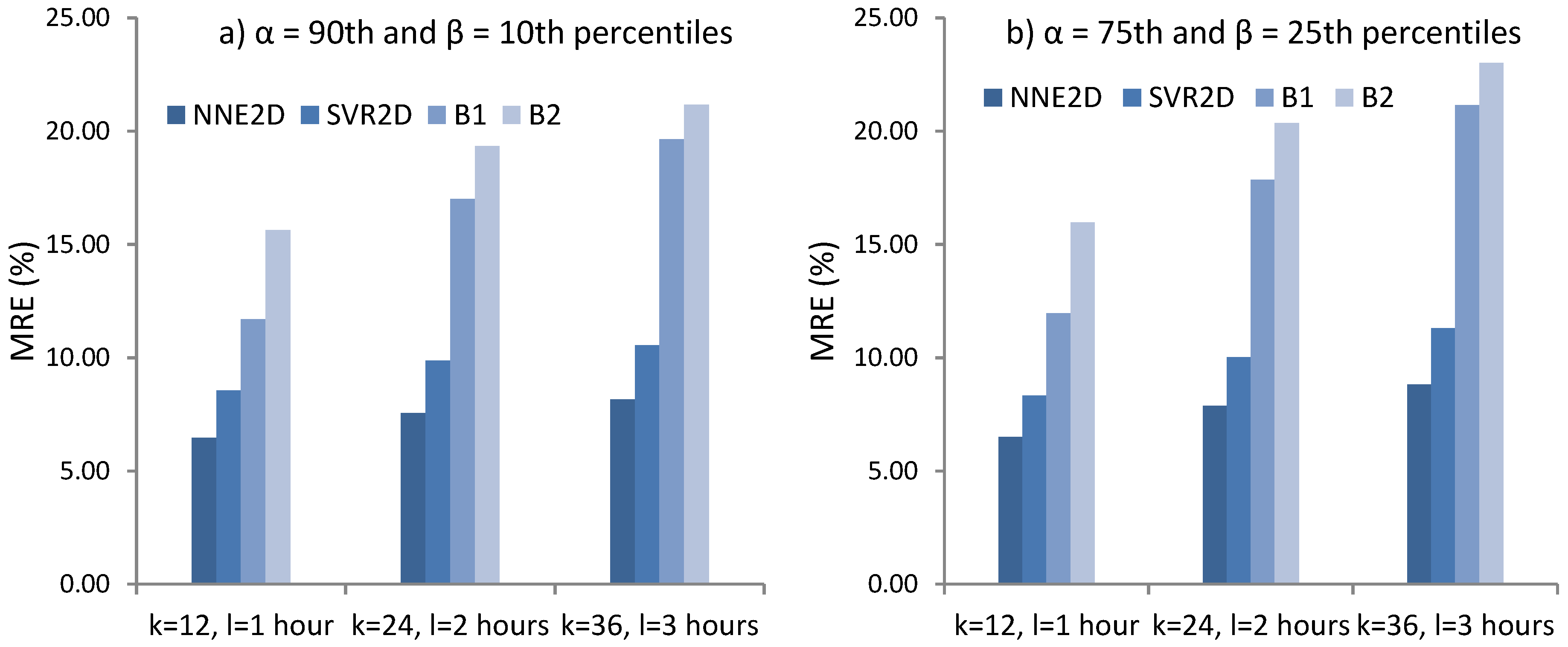
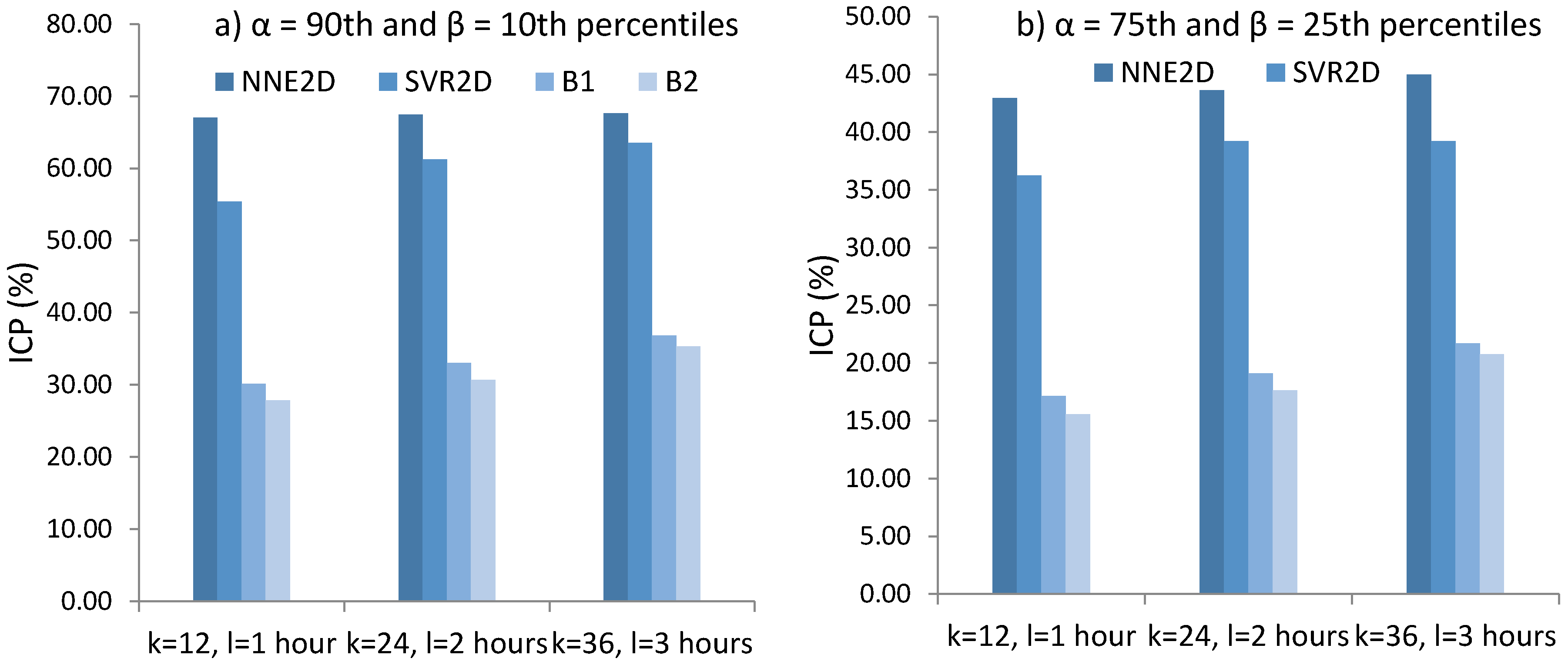
NNE2D was compared with two persistence models used as baselines and a method based on SVR. It achieved MRE of 6.47%–8.16% and coverage probability ICP of 67.04–67.66 for the 10–90th percentiles and MRE of 6.50–8.83 and ICP of 42.96%–45% for the 25–75th percentiles, considerably outperforming the methods used for comparison. NNE2D also showed superior performance when compared to similar but multivariate methods that use both PV power and weather data. This shows that for very-short term forecasting up to 3 h, there is no need to use weather data. In addition, NNE2D was fast to train which makes it suitable for both online and offline training.
Considering both prediction accuracy and the computational requirements, we conclude that NNE2D is a promising approach for 2D-interval forecasts and is viable for practical applications. It can be used to predict other summary statistics for future intervals, not only percentiles, depending on the specific task and forecasting scenarios.
There are several avenues for future work that we will explore. Firstly, we plan to conduct a detailed sensitivity analysis investigating the impact of the relative size of the training, validation and testing sets and the effect of resampling of these sets when evaluating the performance. Secondly, we will examine if the daily periodical component of the PV power (more pronounced for some types of days, e.g., sunny) can be used to improve the results. Thirdly, we will explore alternative data normalization methods, e.g., based on the daily cycle, that consider the sunrise and sunset times and the solar height. Furthermore, we plan to apply our method to other energy time series, in particular wind energy, electricity demand and electricity price.

Author Contributions

Mashud Rana initiated the study and performed the experiments. Irena Koprinska contributed to the methodology. Both authors analysed the results and jointly wrote the paper.

Conflicts of Interest

The authors declare no conflict of interest.

References

  1. Zhang, P.; Li, W.; Li, S.; Wang, Y.; Xiao, W. Reliability assessment of photovoltaic power systems: Review of current status and future perspectives. Appl. Energy 2013, 104, 822–833. [Google Scholar] [CrossRef]
  2. Solar Power Europe. Global Market Outlook for Solar Power 2015–2019. Available online: http://helapco.gr/pdf/Global_Market_Outlook_2015_-2019_lr_v23.pdf (accessed on 12 October 2016).
  3. Climate Commission. The Critical Decade: Australia’s Future-Solar Energy. Available online: http://www.climatecouncil.org.au/uploads/497bcd1f058be45028e3df9d020ed561.pdf (accessed on 12 October 2016).
  4. European Photovoltaic Industry Association. Connecting the Sun-Solar Photovoltaics on the Road to Large Scale Grid Integration. Available online: http://pvtrin.eu/assets/media/PDF/Publications/other_publications/263.pdf (accessed on 12 October 2016).
  5. Antonanzas, J.; Osorio, N.; Escobar, R.; Urraca, R.; Martinez-de-Pison, F.J.; Antonanzas-Torres, F. Review of photovoltaic power forecasting. Sol. Energy 2016, 136, 78–111. [Google Scholar] [CrossRef]
  6. Lorenz, E.; Scheidsteger, T.; Hurka, J.; Heinemann, D.; Kurz, C. Regional PV power prediction for improved grid integration. Prog. Photovolt. 2011, 19, 757–771. [Google Scholar] [CrossRef]
  7. Pelland, S.; Galanis, G.; Kallos, G. Solar and photovoltaic forecasting through post-processing of the global environmental multiscale numerical weather prediction model. Prog. Photovolt. 2013, 21, 284–296. [Google Scholar] [CrossRef]
  8. Yang, D.; Ye, Z.; Lim, L.H.I.; Dong, Z. Very short term irradiance forecasting using the lasso. Sol. Energy 2015, 114, 314–326. [Google Scholar] [CrossRef]
  9. Yang, H.T.; Huang, C.M.; Huang, Y.C.; Huang, Y.S. A weather-based hybrid method for 1-day ahead hourly forecasting of PV power output. IEEE Trans. Sustain. Energy 2014, 5, 917–926. [Google Scholar] [CrossRef]
  10. Urraca, R.; Antonanzas, J.; Alia-Martinez, M.; Martinez-de-Pison, F.J.; Antonanzas-Torres, F. Smart baseline models for solar irradiation forecasting. Energy Convers. Manag. 2016, 108, 539–548. [Google Scholar] [CrossRef]
  11. Pedro, H.T.C.; Coimbra, C.F.M. Assessment of forecasting techniques for solar power production with no exogenous inputs. Sol. Energy 2012, 86, 2017–2028. [Google Scholar] [CrossRef]
  12. Chen, C.; Duan, S.; Cai, T.; Liu, B. Online 24-h solar power forecasting based on weather type classification using artificial neural networks. Sol. Energy 2011, 85, 2856–2870. [Google Scholar] [CrossRef]
  13. Shi, J.; Lee, W.-J.; Lin, Y.; Yang, Y.; Wang, P. Forecasting power output of photovoltaic systems based on weather classification and support vector machines. IEEE Trans. Ind. Appl. 2012, 48, 1064–1069. [Google Scholar] [CrossRef]
  14. Liu, J.; Fang, W.; Zhang, X.; Yang, C. An improved photovoltaic power forecasting model with the assistance of aerosol index data. IEEE Trans. Sustain. Energy 2015, 6, 434–442. [Google Scholar] [CrossRef]
  15. Dong, Z.; Yang, D.; Reindl, T.; Walsh, W.M. A novel hybrid approach based on self-organizing maps, support vector regression and particle swarm optimization to forecast solar irradiance. Energy 2015, 82, 570–577. [Google Scholar] [CrossRef]
  16. Mandal, P.; Madhira, S.T.S.; Hague, A.U.; Meng, J.; Pineda, R.L. Forecasting power output of solar photovoltaic system using wavelet transform and artificial intelligence techniques. Procedia Comput. Sci. 2012, 12, 332–337. [Google Scholar] [CrossRef]
  17. Wang, Z.; Koprinska, I.; Rana, M. Clustering based methods for solar power forecasting. In Proceedings of the International Joint Conference on Neural Networks (IJCNN), Vancouver, BC, Canada, 24–29 July 2016.
  18. Torgo, L.; Ohasi, O. 2D-Interval Predictions for Time Series. In Proceedings of the 17th ACM SIGKDD International Conference on Knowledge Discovery and Data Mining (KDD), Beijing, China, 12–16 August 2012; pp. 787–794.
  19. Chatfield, C. Time-Series Forecasting; Chapman & Hall/CRC: London, UK, 2000. [Google Scholar]
  20. Rana, M.; Koprinska, I.; Agelidis, V.G. 2D-interval forecasts for solar power production. Solar Energy 2015, 122, 191–203. [Google Scholar] [CrossRef]
  21. University of Queensland Solar Data. Available online: http://solar-energy.uq.edu.au/ (accessed on 12 October 2016).
  22. Guyon, I.; Elisseeff, A. An introduction to variable and feature selection. J. Mach. Learn. Res. 2003, 3, 1157–1182. [Google Scholar]
  23. Koprinska, I.; Rana, M.; Agelidis, V.G. Correlation and instance based feature selection for electricity load forecasting. Knowl. Based Syst. 2015, 81, 29–40. [Google Scholar] [CrossRef]
  24. Kraskov, A.; Stögbauer, H.; Grassberger, P. Physical Review E. Estimating mutual information. Phys. Rev. E 2004, 69. [Google Scholar] [CrossRef]
  25. Mellit, A.; Pavan, A.M. A 24-h forecast of solar irradiance using artificial neural network: application for performance prediction of a grid-connected PV plant at Trieste, Italy. Sol. Energy 2010, 84, 807–821. [Google Scholar] [CrossRef]
  26. Koprinska, I.; Rana, M.; Troncoso, A.; Martínez-Álvarez, F. Combining pattern sequence similarity with neural networks for forecasting electricity demand time series. In Proceedings of the International Joint Conference on Neural Networks (IJCNN), Beijing, China, 4–9 August 2013.
  27. Rana, M.; Koprinska, I.; Troncoso, A. Forecasting hourly electricity load profile using neural networks. In Proceedings of the International Joint Conference on Neural Networks (IJCNN), Beijing, China, 6–11 July 2014.
  28. Hippert, H.S.; Pedreira, C.E.; Souza, R.C. Neural Networks for short-term load forecasting: A review and evaluation. IEEE Trans. Power Syst. 2001, 16, 44–55. [Google Scholar] [CrossRef]
  29. Kuncheva, L.I. Combining Pattern Classifiers: Methods and Algorithms; Wiley: Hoboken, NJ, USA, 2014. [Google Scholar]
  30. Rana, M.; Koprinska, I.; Agelidis, V. Univariate and multivariate methods for very short-term solar photovoltaic power forecasting. Energy Convers. Manag. 2016, 121, 380–390. [Google Scholar] [CrossRef]
  31. Nguyen, D.; Widrow, B. Improving the learning speed of a 2-layer neural network by choosing initial values of the adaptive weights. In Proceedings of the International Joint Conference on Neural Networks (IJCNN), Beijing, China, 17–21 June 1990.
  32. Hagan, M.T.; Menhaj, M.B. Training feedforward networks with the Marquardt algorithm. IEEE Trans. Neural Netw. 1994, 5, 989–993. [Google Scholar] [CrossRef] [PubMed]
  33. Zhang, Y.; Beaudin, M.; Zareipour, H.; Wood, D. Forecasting solar photovoltaic power production at the aggregated system level. In Proceedings of the North American Power Symposium (NAPS), Pullman, WA, USA, 7–9 September 2014; pp. 1–6.
  34. Smola, A.J.; Scholkopf, B. A tutorial on support vector regression. Stat. Comput. 2004, 14, 199–222. [Google Scholar] [CrossRef]
  35. Müller, K.R.; Smola, A.J.; Rätsch, G.; Schölkopf, B.; Kohlmorgen, J.; Vapnik, V. Predicting Time Series with Support Vector Machines; Springer: Berlin/Heidelberg, Germany, 1997; pp. 999–1004. [Google Scholar]
  36. Martínez-Álvarez, F.; Troncoso, A.; Asencio-Cortés, G.; Riquelme, J.C. A survey on data mining techniques applied to energy time series forecasting. Energies 2015, 8, 13162–13193. [Google Scholar] [CrossRef]
  37. Setiawan, A.; Koprinska, I.; Agelidis, V.G. Very short-term electricity load demand forecasting using support vector regression. In Proceedings of the International Joint Conference on Neural Networks (IJCNN), Atlanta, GA, USA, 14–19 June 2009; pp. 2888–2894.
  38. Zeng, J.; Qiao, W. Short-term solar power prediction using a support vector machine. Renew. Energy 2013, 52, 118–127. [Google Scholar] [CrossRef]
  39. Rana, M.; Koprinska, I.; Khosravi, A.; Agelidis, V.G. Prediction intervals for electricity load forecasting using neural networks. In Proceedings of the International Joint Conference on Neural Networks (IJCNN), Beijing, China, 4–9 August 2013.
Figure 1. Typical patterns of solar power output under different weather conditions: for a sunny day (13 April 2013), cloudy day (15 April 2013) and rainy day (20 April 2013).
Energies 09 00829 g001
Figure 2. 2D-interval forecast for PV power time series.
Energies 09 00829 g002
Figure 3. Block diagram of the proposed NNE2D approach.
Energies 09 00829 g003
Figure 4. MI score of lag variables for intervals with different length k: (a) k = 12 and (b) k = 24.
Energies 09 00829 g004
Figure 5. Architecture of a single NN in NNE2D.
Energies 09 00829 g005
Figure 6. Ensemble construction and selection for NNE2D.
Energies 09 00829 g006
Figure 7. Comparison of MRE for all methods: (a) α = 90th and β = 10th percentiles, (b) α = 75th and β = 25th percentiles.
Energies 09 00829 g007
Figure 8. Comparison of ICP for all methods: (a) α = 90th and β = 10th percentiles, (b) α = 75th and β = 25th percentiles.
Energies 09 00829 g008
Figure 9. Regression plots of actual and predicted values for the intervals with length 30 min, and α = 90th and β = 10th percentiles.
Energies 09 00829 g009
Figure 10. Intervals with lengths 1 h (k = 12) for a subset of testing data.
Energies 09 00829 g010
Figure 11. Convergence during training of a typical NN in NNE2D.
Energies 09 00829 g011
Table 1. Selected variables to predict P k α and P k β of the k -length interval [ t + 1 ,   t + k ] .
Variable TypesSelected VariablesNumber of Variables
Lag variables X t 5 , X t 4 , X t 3 , X t 2 , X t 1 ,   X t 6
Descriptive statistics of previous k -length interval P k 1 α ,   P k 1 β 2
Total number of variables-8
Table 2. Summary of training, validation and testing data sets.
Data SetPercentage SplitNumber of Samples
Training set50%43,800
Validation set25%21,900
Testing set25%21,900
Total100%87,600
Table 3. Interval lengths and bounds for 2D-interval forecasts.
Interval LengthUpper Bound (α-Percentile)Lower Bound (β-Percentile)
In Steps, kIn Time, l
121 h9010
7525
242 h9010
7525
363 h9010
7525
Table 4. Accuracy results for NNE2D.
Interval LengthLower and Upper Bounds ( α - β Percentiles)Evaluation Metrics
In Steps, kIn Time, lMAID [kW]MRE [%]ICP [%]
121 h10th–90th74.416.4767.04
242 h86.927.5667.46
363 h93.868.1667.66
121 h25th–75th74.726.5042.96
242 h90.537.8743.65
363 h101.538.8345.00
Table 5. Accuracy results for the methods used for comparison: SVR2D, B1 and B2.
Interval LengthLower and Upper Bounds ( α - β Percentiles)Evaluation Metrics
In Steps, kIn Time, lMAID [kW]MRE [%]ICP [%]
SVR2D
121 h10th–90th98.438.5655.38
242 h113.489.8761.24
363 h121.2310.5463.55
121 h25th–75th95.798.3336.25
242 h115.3210.0339.20
363 h130.0011.3039.23
B1
121 h10th–90th134.4411.6930.10
242 h195.5117.0033.01
363 h225.8819.6436.83
121 h25th–75th137.5411.9617.16
242 h205.3417.8519.09
363 h243.3121.1521.72
B2
121 h10th–90th179.8415.6327.86
242 h222.5219.3530.68
363 h243.5821.1835.30
121 h25th–75th183.6715.9715.59
242 h234.2220.3617.65
363 h264.7823.0220.76
Table 6. Comparison of the mean interval width for intervals with different lengths and bounds.
Interval LengthLower and Upper Bounds ( α - β Percentiles)Predicted MIW (kW)Actual MIW (kW)
In Steps, kIn Time, l
121 h10th–90th222.09212.88
242 h308.53298.22
363 h380.00369.74
121 h25th–75th130.33124.59
242 h182.48176.22
363 h226.08219.32
Table 7. Comparison of prediction accuracy for NNE2D, SVR2D ref and NN2D ref .
Interval LengthLower and Upper BoundsNNE2D S V R 2 D r e f N N 2 D r e f
In Steps kIn Time lMAID (kW)MRE (%)ICP (%)MAID (kW)MRE (%)ICP (%)MAID (kW)MRE (%)ICP (%)
121 hmin-max76.656.6674.47100.848.7762.01112.039.7457.10
242 h88.037.6580.17127.0811.0571.01139.2512.1159.53
363 h91.237.9383.08128.0911.1477.78138.3512.0363.86
Average:85.307.4279.24118.6710.3270.27129.8811.2960.16
St. deviation:7.670.674.3815.451.347.9115.461.343.42

