Cost Analysis Method for Estimating Dynamic Reserve Considering Uncertainties in Supply and Demand

Abstract

The use of appropriate hourly reserve margins can maintain power system security by balancing supply and demand in the presence of errors in the forecast demand, generation outages, or errors in the forecast of wind power generation. Because the cost of unit commitment increases with larger reserve margins, cost analysis to determine the most economical reserve margin is an important issue in power system operation. Here, we define the “short-term reliability of balance” and describe a method to determine the reserve margin based on the short-term reliability of balance. We describe a case study, in which we calculate the reserve margin using this method with various standards of short-term reliability of balance. A cost analysis is then performed to determine the most economic standard, and a comparison between our method and a conventional method is carried out. The results show that our method with an economic short-term reliability of balance enables more reliable and efficient operation of the power system. Moreover, with an hourly reserve margin, we show that an increase in wind power generation can result in a significant decrease in the operating cost, which makes wind power generation economically viable.

1. Introduction

One of the most important characteristics of power systems is that demand and supply be balanced at all times. An unexpected change in demand or supply results in fluctuations in the system frequency, and if balance between generation and load is lost, it can lead to frequency deviations, a loss of synchronization between generators, or even a blackout of the entire power system. For this reason, the system operator (SO) should provide operating reserve to account for unexpected fluctuations in demand or supply, or problems that may occur in the electrical grid.

The appropriate operating reserve margin is related to both the reliability and the cost associated with maintaining it. A larger operating reserve margin provides greater ability to accommodate unexpected losses of generators or increases in demand. However, a larger reserve margin also leads to higher generation costs of the reserve generators. Because operating reserve should be available at all times, an excessive operating reserve margin will lead to significant additional costs.

A great deal of discussion has focused on appropriate operating reserve margins, including methods to estimate the frequency regulation reserve [1,2] and consideration of contingencies [3], as well as operating standards for optimal reserve [4,5]. These reports focused on operating reserve margins that apply during time periods greater than one day.

In [1,2,3,4,5], the main uncertainty considered is generation outage, which could result in an insufficient supply of power compared with demand. However, unexpected variations in demand may occur over much shorter timescales, and the required reserve margin will differ for each time period. Therefore, for the SO to manage the power system more economically, the reserve margin should be allowed to vary with time, rather than being fixed for a constant rate of demand all day. Both [6,7] consider the uncertainties in probabilistic outage with expected energy not served (EENS) and estimate an appropriate operating reserve margin that satisfies risk criteria such as the loss of load probability (LOLP). Furthermore, [8,9] also consider the load forecasting error to optimize the spinning reserve requirements while maintaining certain LOLP criteria. In [10], the tradeoff between unit capacity and average production cost is analyzed and the spinning reserve margin is optimized while considering the schedule cost and expected interruption cost. In [11], some indices of credibility assessment are proposed to predict the forecasting error and probabilistic load forecast, which could support decision-making in power system operation. Nonetheless, these papers did not consider instability in supply caused by wind power generation, which could form a significant proportion of the power supply and have a more variable power output than conventional generators.

In addition to the uncertainties caused by generation outage, many investigations have considered uncertainties in wind power forecasting for power systems with a large portion of wind power generation [12,13,14,15,16]. If there is high penetration of wind generation in a power system, the forecasting error cannot be ignored regarding the uncertainties in the supply of power. In [17], wind power uncertainty is modeled explicitly using scenarios, and reserve requirements are enforced on the scenarios to account for the limited number of scenarios represented. A new type of unit commitment, which considers the interruptible load as a reserve to handle the increased uncertainty with wind power, is also suggested in [18]. Both [19,20] also consider wind power generation as an operating risk and propose an algorithm based on non-parametric kernel density estimation and a model for a short-term future forecasting using a conditional probability approach to reduce the risk. In [21,22], wind power uncertainty is modeled as Gaussian distribution and finite-state Markove chain, respectively. Then reserve capacity which could minimize the expected cost is calculated based on each model. However, although these studies considered the uncertainties in wind power generation, they did not fully incorporate other major uncertainties arising from load forecasting and generation outage.

Finally, methods to calculate hourly reserve margins considering the uncertainties of load forecast, generation outage, and wind power generation are researched [23,24,25,26,27]. In [23], the required operating balance reserve is estimated with consideration given to the load forecast error and unavailable capacity due to unit outage in a time horizon of 1–48 h. Both [24,25] generate probability functions of conventional generation outage, load forecasting uncertainty, and wind power forecast uncertainty, and the reserve margin is estimated considering the trade-off between risk and reserve cost. In [26], a new random variable which consists of uncertainties of load shedding and wind curtailment is defined, and conditional value-at-risk (CVaR) is adopted to determine risk reserve requirement. In [27], the spinning reserve margin is determined from a defined term called the short-term reliability of balance, which is calculated from the probabilistic models of uncertainties.

Nevertheless, most papers did not consider the relation between unit commitment and probabilistic generation outage modeling. The most important thing in modeling the uncertainties while considering uncertainties like demand forecasting, generation outage, and wind power forecasting is that they are related and cause differences in the overall demand and supply of power. Specifically, the generation outage should be considered carefully, because the volume of generating output planned to supply the system that cannot be used because of the outage is strongly linked to the result of unit commitment and economic dispatch. The unit commitment and economic dispatch should also be calculated while considering the uncertainties in generation outage when they are dealing with the risk of uncertainties combined with demand forecasting and wind power generation error.

Consequently, algorithms and calculation methods should be developed to consider these uncertainties in the unit commitment and estimating operating reserve margin. Moreover, any estimation of the operating reserve margin should consider not only the risk that an unbalance of supply and demand occurs but also the overall operating cost. Cost analysis should take into account both the generation cost, calculated from the unit commitment and dispatch, and the load-shedding cost, which is related to the risk that the uncertainties would cause, because a greater reserve margin would decrease the risk but increase the generation cost. Therefore, the unit commitment and reserve margin should be estimated to minimize operating costs while maintaining a certain level of risk.

This paper describes a unit commitment method that considers the uncertainties caused by load forecasting, generation outage, and wind power forecasting. An algorithm that considers the generation outage more precisely is included. This algorithm calculates the economic dispatch and estimated reserve margin based on the overall expected cost and amount of risk, which is defined as the short-term reliability of balance. The major contributions of this paper are as follows: (1) precise generation outage modelling is formulated from unit commitment result based on the premise that volume of generation outage occurred equals the volume planned in unit commitment; (2) a new algorithm is proposed that can perform unit commitment with minimum reserve margin constraints in order to maintain the reliability standard in all time period, where the minimum reserve margin constraints are calculated with consideration of demand forecasting and wind power forecasting errors as well as generation outage; and (3) a case study is carried out to identify the usefulness of the proposed method in terms of improved reliability and cost-effectiveness, compared to the conventional method.

The remainder of this paper is organized as follows: Section 2 introduces the probability distribution formulations of uncertainty factors. Demand forecast errors, generation outage, and wind power generation forecast errors are considered in this section along with the short-term reliability of balance to consider these three errors at the same time. In Section 3, the definition of short-term reliability of balance and the algorithm that is used to estimate the dynamic reserve is given. Section 4 describes the formulation of the operating cost, which includes the generation and load-shedding costs. Section 5 describes a case study using the reserve and cost calculation methods, and Section 6 concludes the paper.

2. Probability Distribution Model of Uncertainties in Demand and Supply

2.1. Probability Distribution Model of Demand Forecast Error

The hourly reserve requirement is closely related to the uncertainty in demand, which can be represented by the error associated with the forecast load, and hence by a probability distribution model for demand.

The demand at time t for case s can be calculated as follows [28]:

$$A{D}_t^s=E{D}_t^s+L_t$$

(1)

where $E{D}_t^s$ is the forecast demand at time t for case s and L_t is the error in that forecast demand. Here, we assume that the forecast error in the demand follows a normal distribution with a zero mean [29].

Clearly, a larger error corresponds to a larger standard deviation in the demand. The error varied because the demand pattern of customers differed on both an hourly basis and a seasonal basis. These errors can be described using a statistical approach with data from the forecast peak demand and the actual peak demand, i.e.,

$$T{E}_t=\frac{1}{C_t^s}{\displaystyle \sum _s\frac{\left|A{D}_t^s-E{D}_t^s\right|}{A{D}_t^s}}\times 100(\%)$$

(2)

Assuming that the probability distribution of the demand is normally distributed [30], the difference between the actual demand and the expected demand $A{D}_t^s-E{D}_t^s$, will also follow a normal distribution. Therefore, the absolute value of the difference, |$A{D}_t^s-E{D}_t^s$|, can be described by the positive-valued half of a zero-mean normal distribution. Assuming a sufficiently long time period and the values of $A{D}_t^s$ being similar to each other, the mean of this half-normal distribution can be calculated as follows [31]:

$$E(A{D}_t^s-E{D}_t^s)=\sqrt{\frac{2}{\pi }}{\sigma }_t=\frac{1}{N_t^s}{\displaystyle \sum _s\left|A{D}_t^s-E{D}_t^s\right|}=A{D}_t^s\times \frac{T{E}_t}{100}$$

(3)

Assuming $A{D}_t^s-E{D}_t^s$, we find

$$\sqrt{\frac{2}{\pi }}{\sigma }_t=E{D}_t^s\times \frac{{TE}_t}{100}$$

(4)

The standard deviation in the demand forecast error during hour t is therefore

$${\sigma }_t=\sqrt{\frac{\pi }{2}}\times E{D}_t^s\times \frac{{TE}_t}{100}$$

(5)

and we can conclude that the probability distribution of the hourly forecast error in the demand is normally distributed with a standard deviation given by (5).

2.2. Probability Distribution Model of Generator Outages

The power output of each generator differs from hour to hour due to unit commitment and variations in the load. The uncertainty during peak times, when a large number of generators are online, is larger than that for off-peak times. Accordingly, a different probability distribution is required during peak times and off-peak times. The probability distribution model of generator outages should be calculated using the forced outage rate (FOR) for each generator, which is defined as the probability that the unit will be unavailable under similar conditions [32].

Because the probability distribution model is calculated hourly, the FOR for each generator is defined as the probability that the generator is not available in that hour. The probability that the generator i is available in that hour is therefore given by 1 − FOR_i.

From the results of unit commitment, if a given generator is unavailable, then neither is the power that the generator was planned to provide. It follows that the dispatch schedule and planned power output of generators will change in response to an outage. Because the demand varies as a function of time, the available power will also vary, even though the FOR of generators is constant with the time. Consequently, the probability distribution of outages varied with time.

The time-dependent probability of generator outage G_t can be calculated as follows:

$$P(G_t)={\displaystyle \sum _{j}P(G_{t,j})}$$

(6)

subject to

$$P(G_{t,j})={\displaystyle \prod _{N\in {\mathfrak{F}}_t}{P}_{FOR}^N}$$

(7)

and

$${\mathfrak{F}}_t=\{N|{\displaystyle \sum _{N\in {\mathfrak{F}}_t}{G}_t^N=G_t}\}$$

(8)

These expressions show that an outage G_t occurs when the sum of the outage generators is G_t and can be calculated as the product of the FOR of each generator.

Unlike the probability distribution for demand, the probability distribution for generator outage is discrete and positive-valued because the lack of capacity is determined from the combination of online generators and the planned generation output.

2.3. Probability Distribution Model of Forecast Error for Wind Power Generation

The expected wind power generation may differ on an hourly basis because of fluctuations in the wind velocity and direction. The resulting probability distribution errors in wind power generation vary depending on the expected wind power generation, which can be approximated by a gamma distribution. In order to build a detailed model of the probability distribution of the error in the wind power generation, the expected wind power can be divided into five classes for separate analysis [23].

The results for Classes 1 and 2 have relatively small wind power generation and tend to have a positive error, whereas Classes 4 and 5 have large expected wind power generation and tend to have negative errors in the probability distribution. It follows that if relatively low wind power generation is expected, it is more likely that the expected value will be an underestimate; i.e., the wind forecast error was typically positive. With higher wind power generation, the expected value tended to overestimate the forecast wind power; i.e., the forecast error in the wind power was typically negative.

To approximate the data using a gamma distribution, some modifications are required because a gamma distribution is defined only in the range greater than zero, and the probability density function has an average value of $k\theta$. Assuming that the average error of these probability distributions in each class is equal to zero, a modified gamma-like distribution was constructed using the basic probability density function with a translation of $-k\theta$ on the x-axis. The probability density functions for Classes 1, 2, and 3 were as follows:

$$f(x;k,\theta )=\frac{{(x+k\theta )}^{k-1}{e}^{-(x+k\theta )/\theta }}{{\theta }^k\mathrm{\Gamma }(k)}forx>0,k>0,\theta >0$$

(9)

Classes 4 and 5 exhibit probability distributions that are right-sided. These probability distributions are described by probability density functions that are reflected on the y-axis, so that the probability density functions for Classes 4 and 5 are as follows:

$$f(x;k,\theta )=\frac{{(-x-k\theta )}^{k-1}{e}^{(x+k\theta )/\theta }}{{\theta }^k\mathrm{\Gamma }(k)}forx>0,k>0,\theta >0$$

(10)

3. Algorithm for Dynamic Reserve Estimation

To calculate the hourly reserve using the probability distribution models of the demand forecast error, generation outage and wind power generation errors should be defined; i.e., the “standard” that determines the reserve margin should be defined. Here this “standard” is termed the “short-term reliability of balance” and is calculated from the probability that imbalance between supply and demand occurs in a given hour, considering the uncertainties in supply and demand.

If P_R,t is the reserve for hour t, the probability that imbalance in supply and demand occurs is as follows:

$$P(P_{\mathrm{Im},t}>P_{R,t})=P(G_t+L_t+W_t>P_{R,t})={\displaystyle \sum _{x=0}^{P_{total}}[P(G_t=x)\times P(P_{\mathrm{Im},t}|L_t+W_t>P_{\mathrm{Im},t}-x)]}$$

(11)

and the probability that balance of supply and demand is maintained during an hour, i.e., the short-term reliability of balance is as follows:

$$S{R}_t=[1-P(P_{\mathrm{Im},t}>P_{R,t})]\times 100(\%)$$

(12)

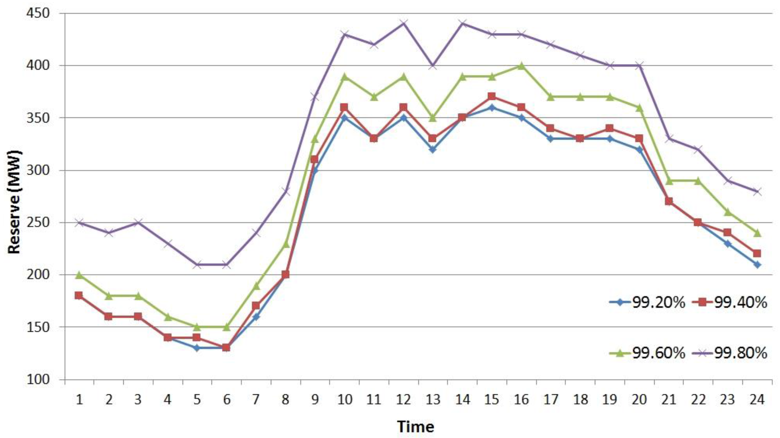
This expression describes the probability that the power system maintains balance between supply and demand if the hourly reserve P_R,t is allocated: the larger the hourly reserve, the larger the SR_t.

To maintain power balance, the short-term reliability of balance should be maintained above a given threshold every hour. If the short-term reliability of balance is determined, the minimum reserve requirement for each hour can be calculated as follows:

$$P_{MR,t}=\min (P_{R,t}:P(P_{\mathrm{Im},t}>P_{R,t})<1-\frac{S{R}_t}{100})$$

(13)

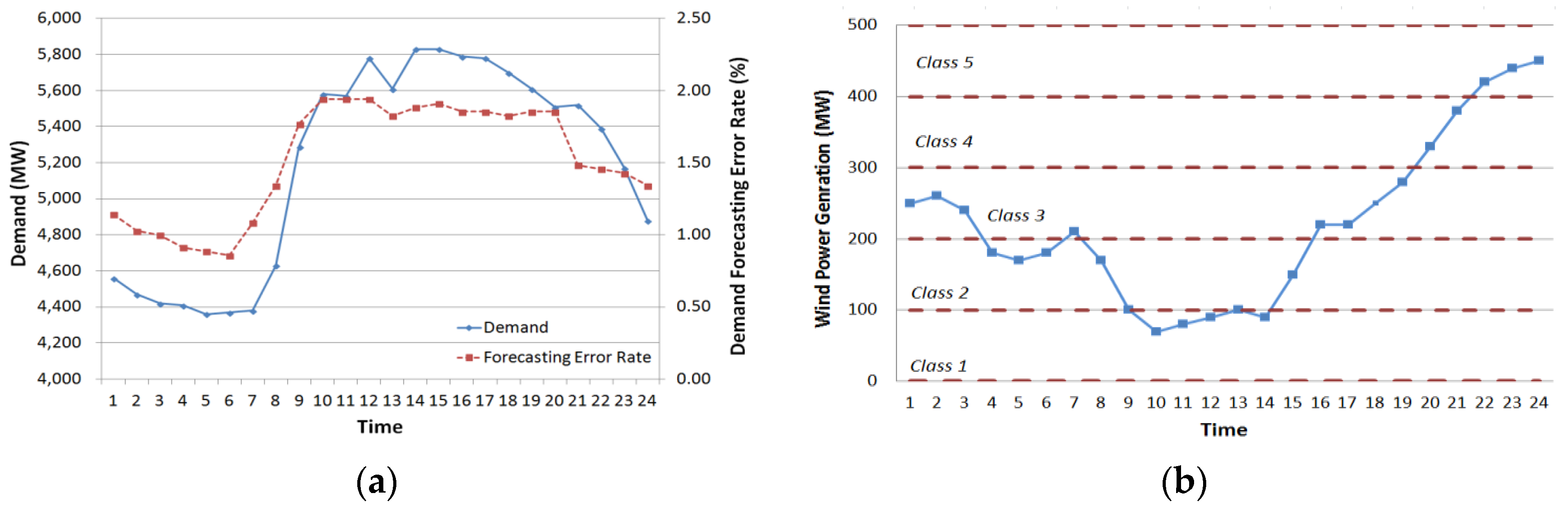
To calculate the reserve requirements for each hour using (13), probability distributions of the error in the forecast demand, generation outages, and the error in the forecast wind power generation should be determined.

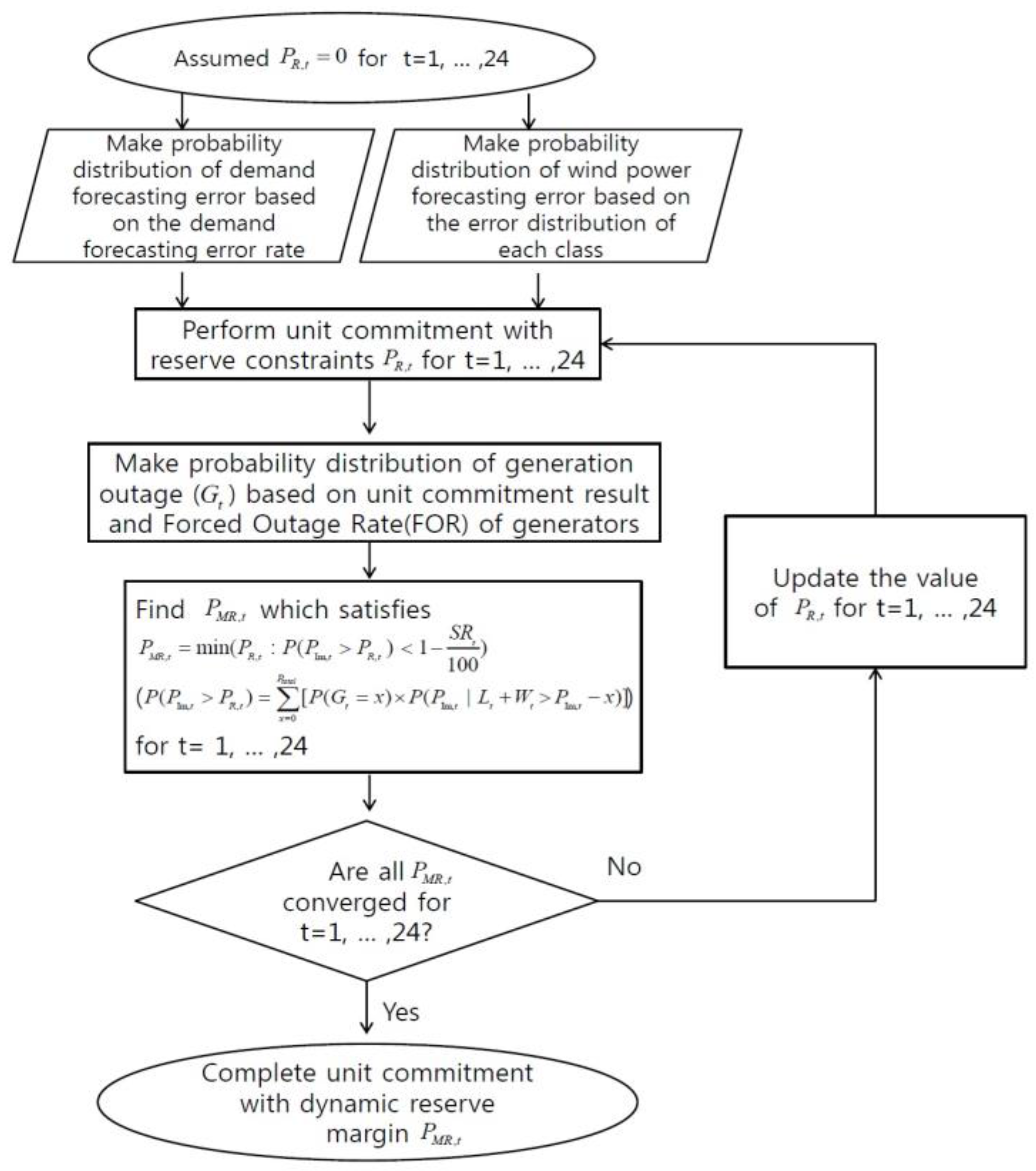
The probability distributions for generator outages are calculated using unit commitment, which provides hourly information on the online/offline status and planned generation for all generators. However, to perform unit commitment, the reserve allocation for each hour should be determined because of the constraints for reserve during each hour, which is part of the unit commitment process. Therefore, to calculate the reserve requirements, a recursive algorithm is used, as shown in Figure 1.

The algorithm in Figure 1 consists of the following four steps:

Step 1.

A probability distribution of the demand forecast error and wind generation forecast error is constructed using data for the hourly demand forecast error and the probability distribution for each class of wind farm.

Step 2.

In the first iteration, the required hourly reserve is assumed to be zero, and unit commitment is carried out with no reserve. A probability distribution for generator outage is then constructed.

Step 3.

The hourly reserve margin is calculated that satisfies (13), and we check for convergence.

Step 4.

If convergence is not achieved, re-enter Step 2 using the calculated reserve requirements from Step 3.

During Step 1, unit commitment is carried out without considering outages of generators, or errors in the forecast demand and wind power. The probability distribution for outrages of generators can be calculated using data from unit commitment; however, these errors cannot be considered in the first iteration. During Step 3, the appropriate reserve margin is calculated using the probability distribution for generator outage, and the errors in the forecast demand and the wind power, which were calculated in Step 2. However, because the required reserve margin changes, the algorithm should be repeated until the hourly reserve margin converges and satisfies both unit commitment and the appropriate reserve margin calculated using (13). When the reserve margin converges, short-term reliability of balance should be satisfied.

4. Cost of Reserve

4.1. Operating Cost

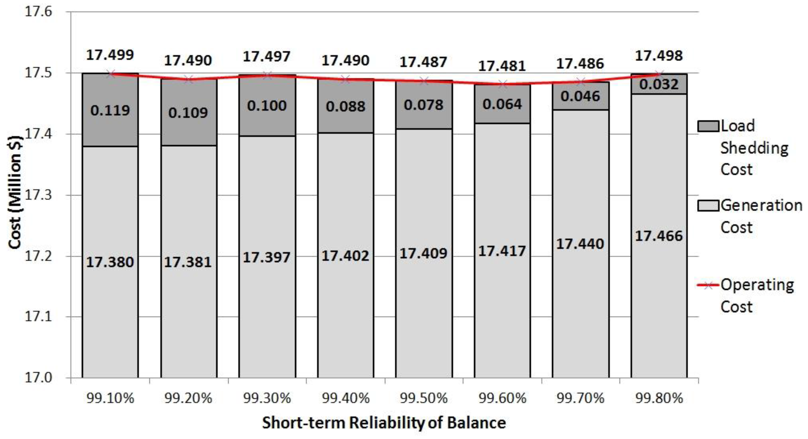
Here, the operating cost is the overall daily cost to maintain power system security, which includes the cost of all conventional generators (i.e., the generation cost), the expected cost for imbalance between demand and supply, and the expected cost of outages (i.e., the load-shedding cost).

As the short-term reliability of balance varies, so will the reserve margin, which results in different generation and load-shedding costs. Therefore, to determine the short-term reliability of balance that is most economical, we should calculate the operating cost as a function of the reserve margin and the short-term reliability of balance for each hour.

4.2. Generation Costs

The generation cost is the cost of conventional generators over 24 h, determined using unit commitment. Unit commitment is the process that determines whether generators are online or offline, and is carried out hourly. The objective is to identify the unit combination that has the lowest cost based on cost functions of each generator, while satisfying the predetermined reserve margin.

The cost function of each generator is a quadratic function of the output of the generators, and is determined by the sum of production cost, which has unit cost coefficients a_i, b_i, and c_i, in each generator and start-up/shutdown cost in terms of generation start-up or shutdown, i.e.,

$$(\mathrm{Generation}\mathrm{Cost})={\displaystyle \sum _{t=1}^{24}[{\displaystyle \sum _{i=1}^{N_G}\{(a_i+b_i{P}_{i,t}+c_i{P}_{i,t}^2)}\times MBtu+ST{C}_i(u_{i,t-1},u_{i,t})\}]}$$

(14)

Because demand is met by both conventional generators and wind power, the generation cost decreases as the wind power penetration increases. Using the method described here to calculate the reserve, the generation cost increases as the short-term reliability of balance increases because the constraints of short-term reliability of balance in unit commitment increase the operating cost.

4.3. Load-Shedding Cost

When imbalance occurs between demand and supply, the SO should carry out load shedding to maintain the system frequency. Those customers affected by load shedding cannot use electricity, and monetary penalties result. The load-shedding cost is the expected sum of these monetary penalties and increases as more load shedding occurs.

Load shedding is determined by the reserve margin and the error in the forecast demand, generation outage, and wind power. The load shedding in hour t, is given by

$$P_{LS,t}=G_t+L_t+W_t-P_{R,t}$$

(15)

and occurs when demand exceeds the sum of the supply and the reserve margin. The probability that load shedding P_LS,t occurs during time t can be calculated as follows:

$$P(P_{LS,t})=P(G_t+L_t+W_t-P_{R,t}=P_{LS,t})={\displaystyle \sum _{x=0}^{P_{Total}}[P(G_t=x)\times P(P_{\mathrm{Im},t}|L_t+W_t=P_{LS,t}-P_{R,t})]}$$

(16)

Using (15) and (16), the load-shedding cost can be calculated as the product of P_LS,t, the probability of load shedding, and the outage cost, C_OC, i.e.,

$$(\mathrm{Load}\mathrm{Shedding}\mathrm{Cost})={\displaystyle \sum _{t=1}^{24}{\displaystyle \sum _{P_{LS,t}=0}^{\infty }\{[{\displaystyle \sum _{x=0}^{P_{Total}}\{P(G_t=x)\times P(P_{\mathrm{Im},t}|L_t+W_t=P_{LS,t}-P_{R,t})\}]\times P_{LS,t}\}\times C_{OC}}}}$$

(17)

Because load shedding decreases as the reserve margin increases, the load-shedding cost also decreases. It follows that the load-shedding cost has an inverse relation with the short-term reliability of balance.

5. Case Study

5.1. Test System Description

A case study was carried out based on an IEEE 118 bus system with 54 generators. The demand and the forecast error in the demand for each hour are shown in Figure 2a. These data were from the summer of 2012 in Korea, and modified proportionally considering the generation capacity of the IEEE 118 bus system. The maximum generation capacity of wind farms was set to 500 MW; the hourly forecast wind power generation is shown in Figure 2b. The probability distributions describing the error in the forecast wind power generation of five classes were determined from the models shown in [23].

The FOR for the 54 generators in the IEEE 118 bus system was divided into 10 (i.e., Type 1 to Type 10), depending on the cost function, and the FOR of each type was set arbitrarily, as listed in

Table 1. Forced Outage Rate (FOR) for the 54 generators in the IEEE 118 bus system.

Type	Unit Number of Generators	Forced Outage Rate (%)
1	4, 5, 10, 29, 36, 40, 43, 44, 45	0.00015
2	7, 14, 16, 19, 22, 23, 26, 34, 35, 37, 47, 48, 51, 52, 53	0.0003
3	33, 41, 46, 49	0.00025
4	20, 21	0.0001
5	1, 2, 3, 6, 8, 9, 12, 13, 15, 17, 18, 31, 32, 38	0.0002
6	11, 39	0.00025
7	59, 61	0.00025
8	42, 50, 54	0.0001
9	27, 28	0.0002
10	30	0.0001

.

The outage cost was assumed to be $2000/MWh. The unit cost coefficients for each generator were taken from the generator data for the IEEE 118 bus system.

5.2. Costs and Optimal Short-Term Reliability of Balance

To determine the most economical short-term reliability of balance, we should minimize the operating cost. In this case study, the hourly reserve margin was calculated to provide a short-term reliability of balance in the range of 99.1%–99.8%. The operating cost is the sum of the generation cost and the load-shedding cost, which was calculated to determine the optimal short-term reliability of balance.

Figure 3 shows the calculated reserve over 24 h to provide a short-term reliability of balance of 99.2%, 99.4%, 99.6%, and 99.8% using (13). The reserve required during each hour increased as the short-term reliability of balance increased, resulting in an increase in the generation costs and a decrease in the load-shedding cost.

Using the methods described in Section 4, the generation and load-shedding costs can be calculated as a function of the short-term reliability of balance, as listed in

Table 2. The calculated costs for various short-term reliabilities of balance in the range 99.1%–99.8%.

Case	Generation Cost ($)	Load-Shedding Cost ($)	Operating Cost ($)
99.1%	1,738,000	11,907	1,749,907
99.2%	1,738,100	10,894	1,748,994
99.3%	1,739,700	9,954	1,749,654
99.4%	1,740,200	8,797	1,748,997
99.5%	1,740,900	7,836	1,748,736
99.6%	1,741,700	6,445	1,748,145
99.7%	1,744,000	4,550	1,748,550
99.8%	1,746,600	3,189	1,749,789

. A minimum in the operating cost corresponded to a short-term reliability of balance of 99.6%, which can therefore be identified as the optimal case.

Figure 4 shows the costs as a function of the short-term reliability of balance. As the short-term reliability of balance increased, so did the generation cost, due to the larger required reserve margin. However, the load-shedding cost decreased as the short-term reliability of balance increased because the increase in the required reserve margin resulted in a smaller probability that demand exceeds supply. The operating cost was minimized for a short-term reliability of balance of 99.6%.

5.3. Comparison of Our Method with a Constant Reserve Margin

To compare the method to calculate the reserve described here with the conventional method, a case study was carried out. The conventional method corresponds to a fixed reserve margin, and the proposed method to a reserve margin that varies from hour to hour with a short-term reliability of balance of 99.6% (i.e., our method). The constant reserve margin for the conventional method was determined using the average reserve margin for the proposed method, which gives the same overall reserve for both cases over 24 h.

Figure 5 shows the reserve allocation result for both cases. The reserve margin of the proposed method was varied to maintain a constant short-term reliability of balance. The case of the conventional method had a fixed reserve margin of 292 MW, which is the rounded value of the 24-h average reserve margin in the case of the proposed method.

Table 3. Maximum, minimum, and mean reserve margins.

Case	Maximum (MW)	Time	Minimum (MW)	Time	Mean (MW)
Conventional method	292	-	292	-	292
Proposed method	400	16	150	5, 6	291.7

lists the average, maximum, and minimum reserve margin for 24 h using the data shown in Figure 6. Because of uncertainties in the forecast demand, the outages of generators and wind power error vary from hour to hour; the times for the maximum and minimum reserve margin depend on the combination of these three uncertain factors.

The short-term reliability of balance was calculated using (12), as shown in Figure 6. Unlike the proposed method, whereby the short-term reliability of balance was maintained >99.6%, the short-term reliability of balance with the conventional method decreased to 97.69%. Furthermore, the time at which the short-term reliability of balance was a minimum was not the same as that for peak demand, which implies that uncertainties in demand forecast error, generation outage, and wind power generation forecast error should be all considered to properly address imbalance.

Table 4. The calculated costs for the conventional method and the proposed method.

Case	Generation Cost ($)	Load-Shedding Cost ($)	Operating Cost ($)
Conventional method	1,737,300	11,681	1,748,981
Proposed method	1,741,700	6,445	1,748,145

lists the calculated costs for the conventional and proposed methods. The operating cost for the proposed method was less than that for the conventional method. The conventional method had a lower generation cost because it was better optimized for unit commitment. As shown in Figure 6, the proposed method required more reserve margin during peak hours, resulting in less optimized unit commitment and a larger generation cost; however, because the reserve allocation for the proposed method was based on the constant short-term reliability of balance, the proposed method has a much lower load-shedding cost than the conventional method. It follows that with the conventional method, a larger probability of imbalance existed between supply and demand. Because the operating cost is the sum of the generation and load-shedding costs, the proposed method (which was based on the calculation method described here) proved to be more cost-effective than the conventional method (a constant reserve margin, as with conventional methods).

5.4. Costs for Different Wind Farms with the Same Short-Term Reliability of Balance

As seen from (11), when the penetration of wind power increases, the corresponding decrease in the use of conventional generators leads to fewer generation outages and G_t would decrease, which decreases the required reserve margin. However, an increase in the penetration of wind power would increase the significance of the error in the forecast wind power generation and increase W_t, leading to an increase in reserve requirements. For this reason, it is possible that, as wind power penetration increases, the operating cost would increase because more reserve margin would be required to maintain a constant level of reliability. This assertion opposes claims that wind power generation is more cost-effective with increasing penetration. Therefore, the overall cost should be analyzed to identify if an increase in wind power penetration would be less cost-effective due to an increase in the operating cost. In this subsection, we describe case studies and analyses of the reserve for various different wind power generation scenarios with the same short-term reliability of balance (i.e., 99.6%). In the simulations, the reserve requirements and costs were calculated as a function of the wind power generation. The wind power generation during each hour was as shown in Figure 2b.

Table 5. Wind power scenarios Case-WT1, Case-WT2, Case-WT3, and Case-WT4.

Case	Number of Wind Farm	Maximum Power (MW)	Wind Power Penetration (%)
Case-WT1	1	500	6.48
Case-WT2	2	1000	12.17
Case-WT3	3	1500	17.20
Case-WT4	4	2000	21.69

lists the four different wind power generation scenarios considered in the simulations. The first, Case-WT1, contained one wind farm with a maximum generation capacity of 500 MW. The other scenarios (i.e., Case-WT2, Case-WT3, and Case-WT4) correspond to two, three, and four wind farms, respectively.

Figure 7 shows the simulated reserve as a function of time using our proposed method. The reserve margin for each hour increased as the wind power generation capacity increased due to the greater significance of the forecast error in the wind power.

Table 6. Simulated costs for scenarios Case-WT1, Case-WT2, Case-WT3, and Case-WT4.

Case	Generation Cost ($)	Load-Shedding Cost ($)	Operating Cost ($)
Case-WT1	1,741,700	6,445	1,748,145
Case-WT2	1,643,700	6,687	1,650,387
Case-WT3	1,549,100	10,758	1,559,858
Case-WT4	1,459,400	16,413	1,475,813

lists the simulated costs for the four wind power generation scenarios. Because more wind power was included with Case-WT4 than Case-WT1, the generation costs were lower. In addition, because the error in the forecast wind generation had a greater impact than the outages of conventional generation, the required reserve margin with Case-WT4 was larger than with Case-WT1 (see Figure 7).

Figure 8 plots the data listed in Table 6. Case-WT4 exhibited the lowest operating cost of the four scenarios. The load-shedding cost increased with increasing wind power penetration due to the greater significance of the wind power forecast error. However, the generation cost (which includes the unit commitment cost while satisfying the required reserve margin calculated for a 99.6% short-term reliability of balance) decreased because of the reduced use of conventional generators, leading to a significant drop in the operating cost as the wind power penetration increased. Although the increased wind power penetration resulted in a larger probability of interruptions to the power system, requiring a larger reserve margin to maintain the same short-term reliability of balance, overall, the increase in wind power penetration reduced the operating cost.

6. Conclusions

We have described a method to calculate the hourly reserve margin considering uncertainties in supply and demand—i.e., generation outages and errors in the forecast demand and wind power. These uncertainties were described using probability distribution models, which were generated for every hour. The reserve margin was calculated hourly based on the short-term reliability of balance, which represents the probability of imbalance between supply and demand. To determine an appropriate short-term reliability of balance that minimizes the operating cost, we consider the generation cost and load-shedding cost.

A case study was carried out using the IEEE 118 bus system to calculate the reserve requirements and costs. The short-term reliability of balance was varied, and the hourly reserve margin was calculated; a cost analysis was then performed to identify the most economical short-term reliability of balance. The reliability and costs were calculated using our method and a conventional method with a fixed reserve margin. The results show that the variable hourly reserve margin (i.e., our method) was both more reliable and more economical. In addition, we carried out a cost analysis with various wind power generation scenarios and showed that the operating cost decreased as the wind power penetration increased.

References

1. Chang-Soo, O.; Kang Wan, L. A study on the requirement of frequency regulation reserve in electricity market. In Proceedings of the Korean Institute of Electrical Engineers Summer Conference, Pyeongchang-gun, Korea, 18 July 2005; pp. 298–300.
2. Chang-Soo, O.; Kang Wan, L. A study on an estimate of frequency regulating reserve. In Proceedings of the Korean Institute of Electrical Engineers Fall Conference, Seoul, Korea, 18 November 2005; pp. 264–266.
3. Hyoung-Yong, S.; Jae-Hyung, R.; Jong-Bae, P.; Joong-Rin, S.; Myung-Suk, C. Optimal dispatch for energy and frequency control reserve considering contingency. In Proceedings of the Korean Institute of Electrical Engineers Summer Conference, Busan, Korea, 14 July 2010; pp. 505–506.
4. Ahn, D.-H.; Kwon, S.-K.; Joo, H.-R.; Choi, E.-J. A research of optimum supply reserve levels for stability of power system. J. Korean Inst. Illum. Electr. Install. Eng. 2008, 22, 55–61. [Google Scholar]
5. Seong-Ho, R.; Kang-Wan, L.; Gwang-Won, K.; Kab-Ju, H. A study on operation standards for optimal operating reserve in electricity market. Trans. Korean Inst. Electr. Eng. A 2003, 52, 287–293. [Google Scholar]
6. Chattopadhyay, D.; Baldick, R. Unit commitment with probabilistic reserve. In Proceedings of the 2002 IEEE Power Engineering Society Winter Meeting, New York, NY, USA, 27–31 January 2002; Volume 281, pp. 280–285.
7. Georgopoulou, C.A.; Giannakoglou, K.C. Metamodel-assisted evolutionary algorithms for the unit commitment problem with probabilistic outages. Appl. Energy 2010, 87, 1782–1792. [Google Scholar] [CrossRef]
8. Ortega-Vazquez, M.A.; Kirschen, D.S.; Pudjianto, D. Optimising the scheduling of spinning reserve considering the cost of interruptions. IEE Proc. Gener. Transm. Distrib. 2006, 153, 570–575. [Google Scholar] [CrossRef]
9. Ortega-Vazquez, M.A.; Kirschen, D.S. Optimizing the spinning reserve requirements using a cost/benefit analysis. IEEE Trans. Power Syst. 2007, 22, 24–33. [Google Scholar] [CrossRef]
10. Wang, M.Q.; Gooi, H.B.; Han, X.S. A tradeoff between unit capacity and average production cost in spinning reserve optimization. Int. J. Electr. Power Energy Syst. 2015, 71, 215–221. [Google Scholar] [CrossRef]
11. Dany, G. Power reserve in interconnected systems with high wind power production. In Proceedings of the 2001 IEEE Porto Power Tech Proceedings, Porto, Portugal, 10–13 September 2001; Volume 4, p. 6.
12. Zhang, Z.; Li, C.; Cao, Y.; Tang, L.; Li, J.; Wu, B. Credibility assessment of short-term load forecast in power system. In Proceedings of the IEEE PES Innovative Smart Grid Technologies, Washington, DC, USA, 16–20 January 2012; pp. 1–5.
13. Doherty, R.; O’Malley, M. A new approach to quantify reserve demand in systems with significant installed wind capacity. IEEE Trans. Power Syst. 2005, 20, 587–595. [Google Scholar] [CrossRef]
14. Saez-Gallego, J.; Morales, J.M.; Madsen, H.; Jónsson, T. Determining reserve requirements in dk1 area of nord pool using a probabilistic approach. Energy 2014, 74, 682–693. [Google Scholar] [CrossRef]
15. Zhou, W.; Sun, H.; Peng, Y. Risk reserve constrained economic dispatch model with wind power penetration. Energies 2010, 3, 1880–1894. [Google Scholar] [CrossRef]
16. Chen, J.; Wu, W.; Zhang, B.; Wang, B.; Guo, Q. A spinning reserve allocation method for power generation dispatch accommodating large-scale wind power integration. Energies 2013, 6, 5357–5381. [Google Scholar] [CrossRef]
17. Ruiz, P.A.; Philbrick, C.R.; Sauer, P.W. Wind power day-ahead uncertainty management through stochastic unit commitment policies. In Proceedings of the 2009 IEEE/PES Power Systems Conference and Exposition, Seattle, WA, USA, 15–18 March 2009; pp. 1–9.
18. Park, H.-G.; Lyu, J.-K.; Kang, Y.; Park, J.-K. Unit commitment considering interruptible load for power system operation with wind power. Energies 2014, 7, 4281–4299. [Google Scholar] [CrossRef]
19. Liao, G.; Ming, J.; Wei, B.; Xiang, H.; Ai, N.J.P.; Dai, C.; Xie, X.; Li, M. Wind power prediction errors model and algorithm based on non-parametric kernel density estimation. In Proceedings of the 2015 5th International Conference on Electric Utility Deregulation and Restructuring and Power Technologies, Changsha, China, 26–29 November 2015; pp. 1864–1868.
20. Thapa, S.; Karki, R.; Billinton, R. Operating risk considerations in wind integrated power systems. In Proceedings of the 2014 International Conference on Probabilistic Methods Applied to Power Systems (PMAPS), Durham, UK, 7–10 July 2014; pp. 1–6.
21. Hedayati-Mehdiabadi, M.; Zhang, J.; Hedman, K.W. Wind Power Dispatch Margin for Flexible Energy and Reserve Scheduling With Increased Wind Generation. IEEE Trans. Sustain. Energy 2015, 6, 1543–1552. [Google Scholar] [CrossRef]
22. Wu, J.; Zhang, B.; Deng, W.; Zhang, K. Application of Cost-CVaR model in determining optimal spinning reserve for wind power penetrated system. Int. J. Electr. Power Energy Syst. 2015, 66, 110–115. [Google Scholar] [CrossRef]
23. Menemenlis, N.; Huneault, M.; Robitaille, A. Computation of dynamic operating balancing reserve for wind power integration for the time-horizon 1–48 hours. IEEE Trans. Sustain. Energy 2012, 3, 692–702. [Google Scholar] [CrossRef]
24. Matos, M.A.; Bessa, R.J. Setting the operating reserve using probabilistic wind power forecasts. IEEE Trans. Power Syst. 2011, 26, 594–603. [Google Scholar] [CrossRef]
25. Liu, G.; Tomsovic, K. Qunatifying Spinning Reserve in Systems With Significant Wind Power Penetration. IEEE Trans. Power Syst. 2012, 27, 2385–2393. [Google Scholar] [CrossRef]
26. Wang, M.; Bai, H.; Zhou, M.; Wang, J. A generation-reserve co-optimization dispatching model for wind power integrated power system based on risk reserve constraints. In Proceedings of the International Conference on Renewable Power Generation, Beijing, China, 17–18 October 2015; pp. 1–6.
27. Kwon, K.-B.; Park, H.-G.; Lyu, J.-K.; Kim, Y.-C.; Park, J.-K. Dynamic reserve estimating method with consideration of uncertainties in supply and demand. Trans Korean Inst. Electr. Eng. 2013, 62, 1495–1504. [Google Scholar] [CrossRef]
28. Ortega-Vazquez, M.A.; Kirschen, D.S. Estimating the spinning reserve requirements in systems with significant wind power generation penetration. IEEE Trans. Power Syst. 2009, 24, 114–124. [Google Scholar] [CrossRef]
29. Bo, R.; Li, F. Probabilistic lmp forecasting considering load uncertainty. IEEE Trans. Power Syst. 2009, 24, 1279–1289. [Google Scholar]
30. Jong-Uk, L.; Young-Min, W.; Sung-Kwan, J.; Kyung-Bin, S.; Jeong-Do, P.; Burm-Sup, C.; Ki-Jun, S. Analysis of load forecasting error for improving the accuracy of the short-term load forecasting. In Proceedings of the Korean Institute of Electrical Engineers Fall Conference, Cheonan-si, Korea, 11 December 2010; pp. 171–172.
31. The Half-Normal Distribution Method for Measurement Error: Two Case Studies. Available online: https://www-users.york.ac.uk/~mb55/talks/halfnor.pdf (accessed on 1 August 2016).
32. Billiinton, R.; Allen, R.N. Generating capacity—Basic probability methods. In Reliability Evaluation of Power Systems; Springer: New York, NY, USA, 1996; pp. 46–47. [Google Scholar]
Figure 1. Solution method to determine the hourly spinning reserve margin.
Energies 09 00845 g001
Figure 2. Forecast demand and wind power generation used in the case study: (a) Forecast demand (labeled with left y-axis) and the error in the forecast demand (labeled with right y-axis) based on data for summer 2012 in Korea; (b) Hourly forecast wind power generation in a typical day and for Classes 1–5.
Energies 09 00845 g002
Figure 3. Hourly reserve margin with the short-term reliability of balance varied from 99.2% to 99.8%.
Energies 09 00845 g003
Figure 4. The generation costs and the cost for interruption as a function of the short-term reliability of balance.
Energies 09 00845 g004
Figure 5. Hourly reserve margins for the conventional method (a fixed reserve margin of 292 MW) and the proposed method (based on a short-term reliability of balance of 99.6%).
Energies 09 00845 g005
Figure 6. Hourly reliability based on the balance of supply and demand.
Energies 09 00845 g006
Figure 7. Hourly reserve margin of case-WT1, Case-WT2, Case-WT3, and Case-WT4.
Energies 09 00845 g007
Figure 8. Calculated costs for scenarios Case-WT1, Case-WT2, Case-WT3, and Case-WT4.
Energies 09 00845 g008