Modeling of a Pouch Lithium Ion Battery Using a Distributed Parameter Equivalent Circuit for Internal Non-Uniformity Analysis

Abstract

A battery model that has the capability of analyzing the internal non-uniformity of local state variables, including the state of charge (SOC), temperature and current density, is proposed in this paper. The model is built using a set of distributed parameter equivalent circuits. In order to validate the accuracy of the model, a customized battery with embedded T-type thermocouple sensors inside the battery is tested. The simulated temperature conforms well with the measured temperature at each test point, and the maximum difference is less than 1 °C. Then, the model is applied to analyze the evolution processes of local state variables’ distribution inside the battery during the discharge process. The simulation results demonstrate drastic distribution changes of the local state variables inside the battery during the discharge process. The internal non-uniformity is originally caused by the resistance of positive and negative foils, while also influenced by the change rate of open circuit voltage and the total resistance of the battery. Hence, the factors that affect the distribution of the local state variables are addressed.

1. Introduction

The lithium ion battery is one of the most promising candidates for the energy storage system (ESS) in electrical vehicles. To reduce the cost, prolong the life and ensure the safety of the ESS, the optimal design of the battery cell and pack with robust battery management system (BMS) is essential. Two kinds of battery models are proposed to fulfill the optimal design and to be implanted in the BMS, respectively. The first kind of model is physics based. A model based on the theory of intercalation electrodes and concentrated solutions was proposed by Doyle et al. [1]. Lou et.al. [2] built an extended single particle model for higher rates simulation. Kim et al. [3,4] developed a multi-scale multi-domain model framework, which resolved electrochemical, thermal and electrical coupled physics at varied length scales in the lithium ion battery. Three-dimensional electrochemical-thermal models were proposed and widely used by researchers [5,6,7,8] to analyze heat generation and temperature distribution in the lithium ion battery. A two-dimensional model was reported by Shin’s group [9,10,11] for the thermal behavior and scale-up design of the lithium-polymer battery. These models are usually computationally complex and time consuming. In addition, a large number of parameters is needed for model inputs, and some of the parameters are extremely hard to obtain. Thus, such models are only suitable for cell designing and analyzing. For example, a three-dimensional electrochemical model was proposed by Kohneh et al. [12] and used to examine the effect of parameters, such as current collector thickness and tab location, on reducing non-uniform voltage and current distribution in the cell. Liu et al. [13] developed an integrated computational method that considered the mechanical, electrochemical and thermal behaviors of the lithium ion battery to study the nail penetration problem. Samba et al. [14] used the electrical-thermal model to design the battery thermal management system. Though simplified approaches, such as the simplified electrochemical multi-particle model and homogenous pseudo two-dimensional model, were developed by Mastali et al. [15] to decrease the computational time, the speed and simplicity of three-dimensional electrochemical-thermal models are still of concern. The second kind of models is the equivalent circuit model (ECM). Here [16,17,18,19,20], the battery is usually regarded as a mass point. Only a few parameters are in the model and can be derived from the external characteristics of the cell [21,22]. Therefore, they are suitable to be implanted in the battery management system (BMS) for the state of charge or the state of health estimation [23,24,25,26]. Lumped-parameter thermal models were added to ECM to predict the thermal characteristics of the cell by Lin et al. [27] and Forgez et al. [28], which made the model more comprehensive.

Meanwhile, in order to reach higher power and energy density, the size of the battery cell is growing. This leads to the imbalance of the potential, current density, temperature and state of charge (SOC) becoming significant, so the battery can no longer be treated as a mass point. Large SOC differences up to 5.3% were reported by Fleckenstein et al. [29] in a LiFePO${}_4$ cell. Taking the computational cost into consideration, a new model to predict the internal imbalance of the battery is desired at this stage. Therefore, the distributed parameter equivalent circuit model (DPECM) is proposed in our former works [30]. However, the former proposed model could only solve the electric related variables, and the model is only validated by the terminal voltage. As the temperature of lithium ion batteries is vital for their life span, safety and performance, thermal models need to be established and implemented into the former proposed model, to analyze the distribution and variation trend of internal current, voltage and temperature.

On the other hand, the validation of those models that could obtain the internal variables is somehow technically difficulty, because the distribution of the internal potential, current density or SOC cannot be measured directly. Wang’s group [31,32] proposed an in situ measurement method for current distribution in a lithium ion battery. The structure of the cell was changed because the positive electrode was segmented along the length of the electrode sheet; while temperature is much easier to measure compared to other variables inside a battery. Forgez et al. [28] and Li et al. [33] successfully embedded thermocouples into cylindrical and pouch cells, respectively. They proved that the cell characteristics affected by the embedded sensors were negligible. To validate the proposed model in our research, a customized cell with nine T-type thermocouples embedded inside the battery was provided by the battery manufacture. The customized battery was tested for the parameter identification and validation of the temperature distribution inside the battery.

The remaining parts of this paper are arranged as follows. Section 2 describes the experimental setup, cell dimensions and temperature sensor locations. Section 3 introduces the modeling method and validation. The internal non-uniformity is discussed in Section 4. The conclusions are summarized in Section 5.

2. Experiments

The cell studied in this paper is a 35 Ah $\mathrm{LiN}{\mathrm{i}}_{1/3}\mathrm{C}{\mathrm{o}}_{1/3}\mathrm{M}{\mathrm{n}}_{1/3}{\mathrm{O}}_2$ (NCM) pouch cell, which has a total of 36 laminated layers. Each laminated layer is composed of positive foil, positive material, separator, negative material, and negative foil, and the characteristics of each component are presented in

Table 1. Properties of each battery component.

Component	Thickness	Heat Conductivity Coefficient	Specific Heat Capacity	Electrical Resistivity
	(μm)	(w·m${}^{-1}$·k${}^{-1}$)	(J·kg${}^{-1}$·k${}^{-1}$)	(Ω·m)
Positive foil	20	238	903	$2.83\times {10}^{-8}$
Positive material	160	3.9	839	—
Separator	40	0.33	1978	—
Negative material	110	3.3	1064	—
Negative foil	10	398	385	$1.75\times {10}^{-8}$

. The top view from cell thick direction and the cell dimensions are shown in Figure 1. The length and width of the main body are 195 mm and 165 mm, respectively. Positive and negative tabs locate at two opposite sides of the cell, whose length and width are 40 mm and 80 mm, respectively. The total thickness of the cell is only 14 mm, which is much smaller than the length and width of battery, so the differences of local SOC, current density, and potential along thick direction are ignored in this paper. In order to acquire internal temperature reliably, nine T-type thermocouples are embedded inside the cell during the manufacturing process of the cell using the same method proposed by Li et al. [33]. The thermocouples were sandwiched by two pieces of separators and then placed in the middle of the thickness before vacuuming and sealing of the cell. Nine thermocouples are uniformly distributed on the middle plane.

In order to obtain the model input parameters and verify the accuracy of the model, two sets of experiments are executed. One is for parameter estimation, and the other is for validation.

2.1. Parameters Identification Experiments

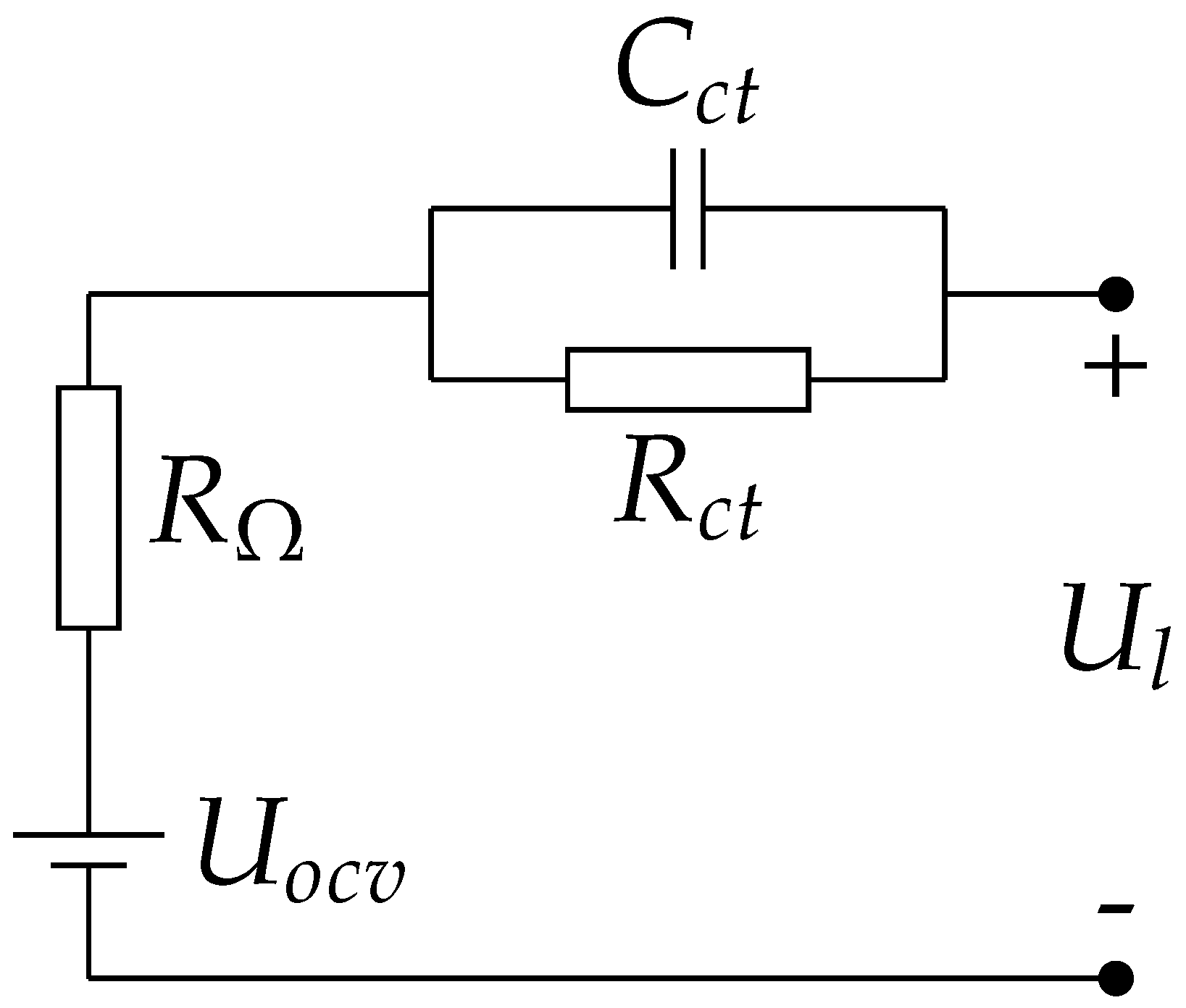
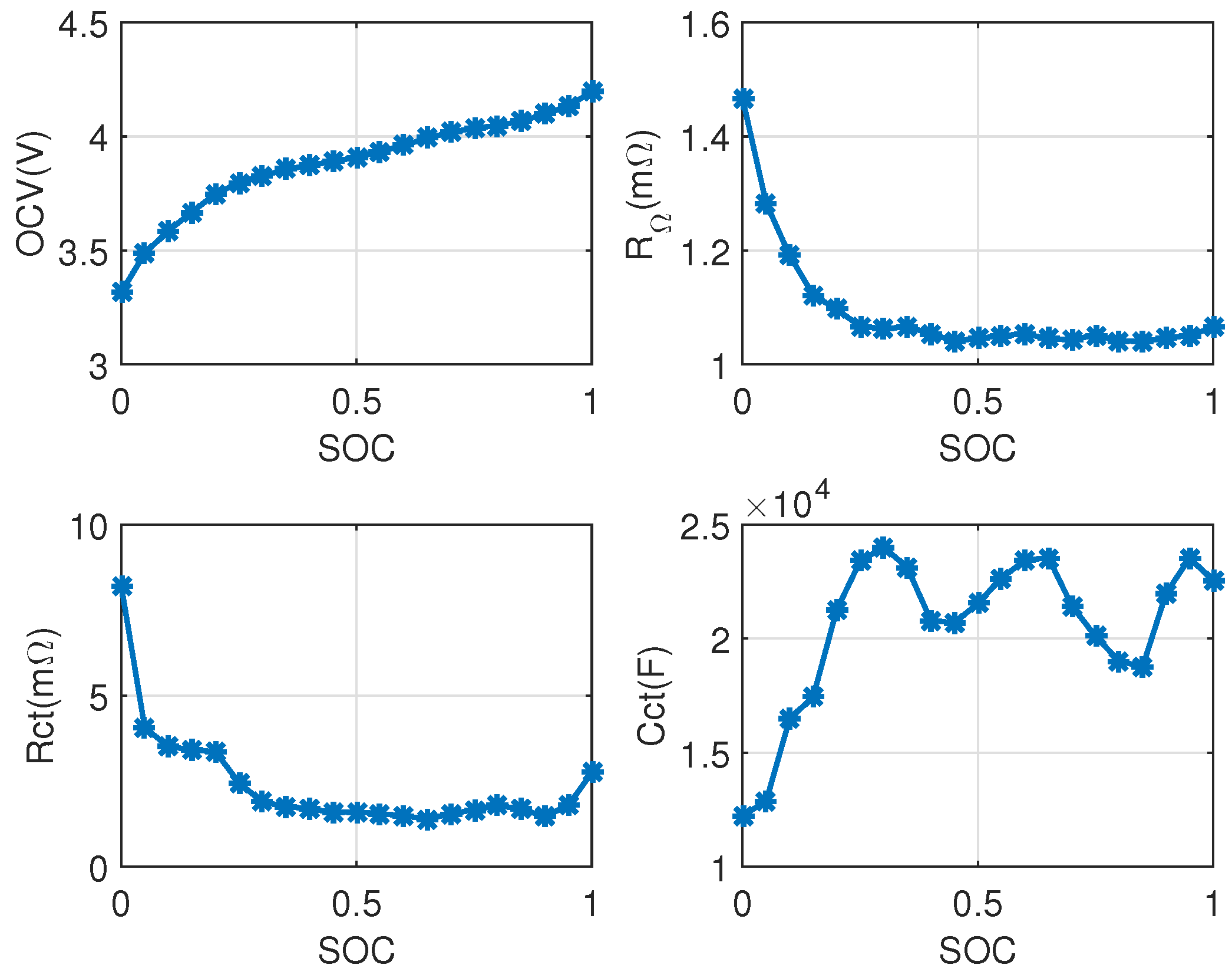
2.1.1. Parameters Identification of the Lumped First-Order Resistor-Capacitor (RC) Model

A typical lumped first-order resistor-capacitor (RC) model is shown in Figure 2. It consists of a voltage source, a resistor and a parallel branch of the resistor and capacitor. The voltage source represents the open circuit voltage (OCV) of the cell. Resistor $R_{\Omega }$ represents the ohmic resistance in the cell. The parallel branch is utilized to model the chemical diffusion in the cell. In order to obtain the parameters of the first-order RC lumped model, pulse discharge is a widely-used method for lithium ion batteries. In this paper, the cell was put into an environment chamber during the test to keep the ambient temperature constant, and then, discharge pulses were applied to the cell by battery test equipment: Arbin BT-2000. Each discharge pulse depleted 5% of the total capacity and was followed by 2 hours of rest. To make the parameters suitable for different current rates, the discharge pulse at each SOC contained multiple current rates, including the current fragments of 0.5C, 1C and 2C, as shown in Figure 3a. The corresponding voltage response of the cell is shown in Figure 3b.

The lumped first-order RC model parameters can be estimated according to the current and voltage curve using the method proposed by Huria et al. [34,35]. The parameters were determined using the parameter estimation tool in Simulink Design Optimization. The tool iteratively simulated the discharge voltage profile while comparing the simulation results with experimental data. The nonlinear least squares algorithm was used to minimize the sum of square error. The fitting result of the discharge pulse at SOC = 0.55 is presented in Figure 4. The fitted results agree well with the experimental data. The estimated parameters of $U_{ocv}$, $R_{\Omega }$, $R_{ct}$ and $C_{ct}$ are shown in Figure 5.

2.1.2. Entropy Change Measurement

The entropy change of the lithium ion battery can describe the generated reversible heat. It can be calculated using Equation (1):

$$\Delta S=F\frac{\mathrm{d}U}{\mathrm{d}T}$$

(1)

where $\Delta S$ is the entropy change of the battery; F is the Faraday constant; U is the equilibrium potential of the battery; T is the temperature.

The entropy change could be calculated through the OCV variation with temperature. The method proposed by Forgez et al. [28] was used in this paper to obtain the coefficient of OCV variation with temperature. The cell was discharged to an objective SOC and rested to the steady state. Then, the temperature of the environment chamber was changed to different values, as shown in Figure 6a. In order to extract the temperature coefficient from these data, the voltage was fitted by the function $V(t,T)=A+BT+Ct$ with A, B and C as constants and B corresponding to the temperature coefficient $\partial U/\partial T$. The fitting results for $\partial U/\partial T$ estimation are shown in Figure 6b. The $\partial U/\partial T$ results are shown in Figure 7.

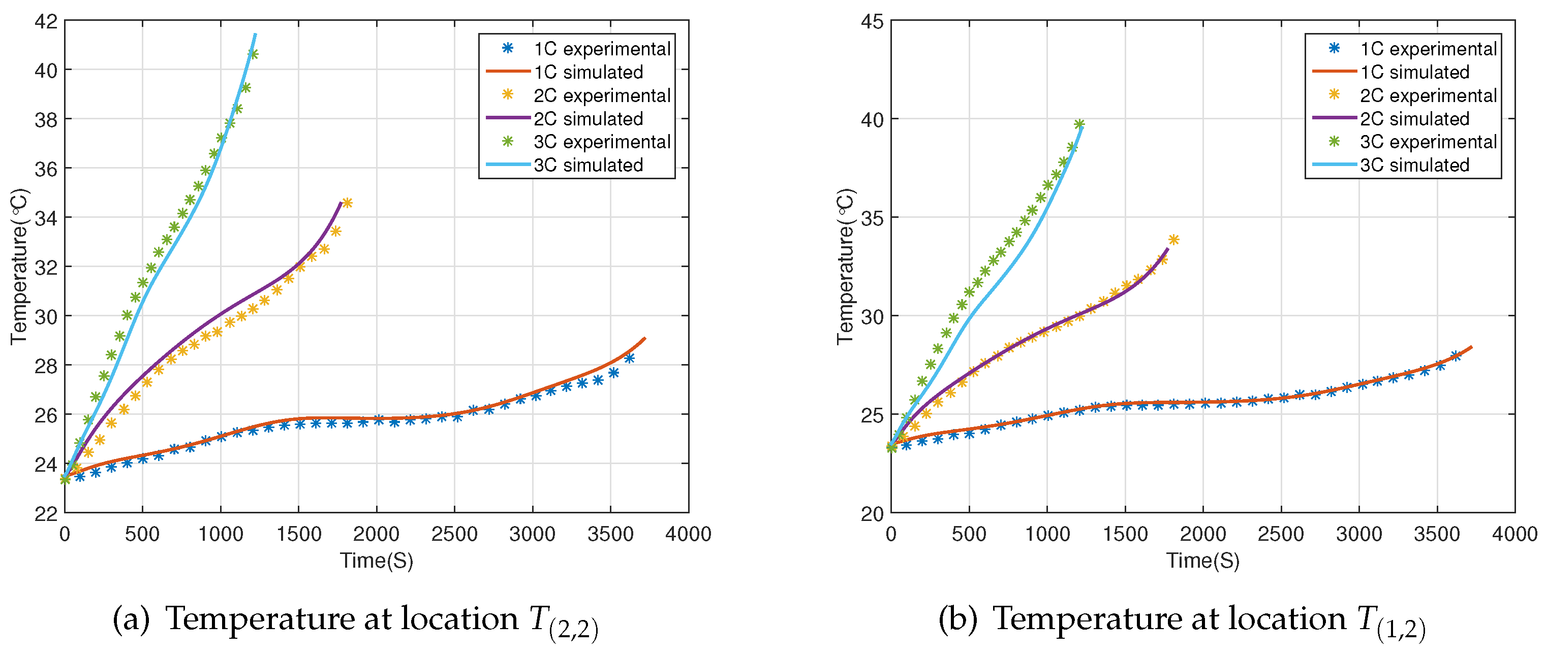
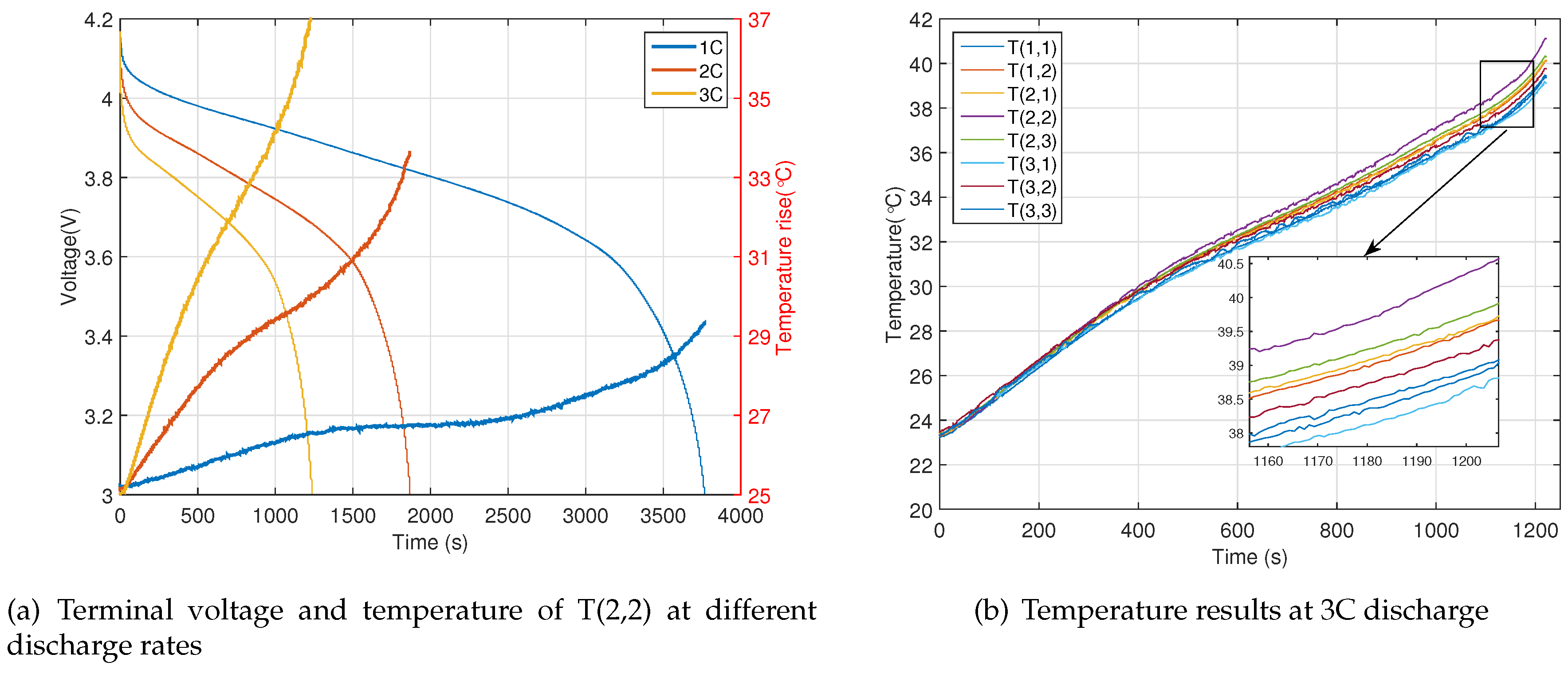
2.2. Validation Experiments

In order to analyze the voltage and temperature characteristics, constant current discharge at 1C, 2C and 3C rates was performed using Arbin BT-2000. The temperature was measured by an Agilent 34901A. The voltage and temperature during the discharge process with different rates are shown in Figure 8a. Figure 8b shows the temperature measured by the internal thermocouples. The thermocouples at T(1, 1) were broken, so the data are not shown here. At the end of discharge, temperature at the center of the cell (T(2, 2)) is the highest. The center temperature close to the positive tab (T(1, 2)) is higher than that close to the negative tab (T(3, 2)), which might be caused by the different properties of positive and negative tabs. Although the geometries of positive and negative tabs are the same, the positive aluminum tab has a smaller heat conductivity coefficient and larger electrical resistivity compared to the negative Copper tab. Therefore, more heat is accumulated around the positive tab, leading to a higher temperature around positive tab. The temperature values of T(2, 1) and T(2, 3) are almost the same, owning to the symmetric cell structure.

3. Modeling and Validation

The model is comprised of two parts. One is the electrical part, which is used to solve the electrical-related variables, such as the potential, current density and SOC. The other is the thermal part to solve the thermal-related variables, including heat generation, conduction and dissipation.

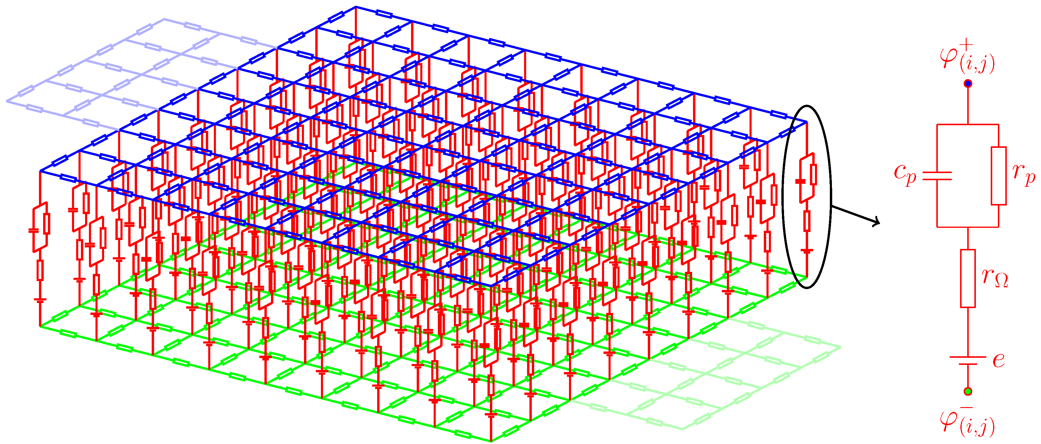
3.1. Electrical Model

The schematic of the electrical part in DPECM is shown in Figure 9. According to the layered structure and electrochemical principles of pouch batteries [36,37,38], the proposed model consists of five parts, including the positive and negative tabs, the positive and negative foils and the main material body. The current flow of positive and negative tabs only exists in the horizontal plate. The positive and negative foils not only have current flowing in the horizontal plate, but also have current pouring into or pumping out from the sub-models. The main material body, including the positive and negative materials, electrolyte and separator, etc., is divided into a group of sub-models. Each sub-model is represented by a first-order RC equivalent circuit. The first-order RC model is adopted in this paper, because Hu et al. [39] indicated that the first-order RC equivalent circuit model was the most suitable candidate for an NCM cell after comparing twelve battery models. One branch of the sub-models was magnified in the right side of Figure 9 to show the details of first-order RC model. It consists of a voltage source, a resistor and a parallel branch of the resistor and capacitor.

The current of the sub-model located at the i-th row and j-th column in Figure 9 could be calculated as Equation (2):

$$i_{(i,j)}=\frac{e_{(i,j)}-({\phi }_{(i,j)}^{+}-{\phi }_{(i,j)}^{+})-u_{p(i,j)}}{r_{\Omega (i,j)}}$$

(2)

where the subscript $(i,j)$ represents the node location; i is the current of the sub-model; e is the equilibrium potential of the sub-model; ${\phi }^{-}$ is the node potential on the negative foil connected with the sub-model; ${\phi }^{+}$ is the node potential on the positive foil connected with the sub-model; $r_{\Omega }$ is the ohmic resistance of the sub-model; $u_p$ is the polarization voltage of the sub-model, which could be calculated as:

$$c_p\frac{\mathrm{d}{u}_p}{\mathrm{d}t}=i-\frac{u_p}{r_p}$$

(3)

where $u_p$ is the initial polarization voltage; $r_p$ is the polarization resistance of the sub-model; $c_p$ is the polarization capacitor of the sub-model. The resistance value $r_p$ in the sub-model is calculated using the equivalent resistance of the lumped first-order RC model multiplied by sub-model numbers. The capacitance value $c_p$ in the sub-model is calculated using the equivalent capacitance of the lumped first-order RC model divided by sub-model numbers.

In this paper, $u_p$ is iteratively updated. Therefore, Equation (3) needs to be discretized. The discretized result of Equation (3) using the Euler method is:

$$u_{p,t+\Delta t}=u_{p,t}+\frac{i_t{r}_{p,t}-u_{p,t}}{r_{p,t}{c}_{p,t}}\Delta t$$

(4)

where $\Delta t$ is the step time; $u_{p,t}$ is the polarization voltage at instant t; $u_{p,t+\Delta t}$ is the polarization voltage at instant $t+\Delta t$; $r_{p,t}$, $c_{p,t}$ and $i_t$ are the polarization resistance, polarization capacitance and current of the sub-model at instant t, respectively.

Assume that there are N nodes in total on the positive foil and tab, as shown in Figure 9. According to Kirchhoff’s current law, the sum of currents flowing through each node is zero. Therefore, a typical node equation is:

$$\begin{array}{cc}{i}_{(i,j)}=\hfill & ({\phi }_{(i-1,j)}^{+}-{\phi }_{(i,j)}^{+})/r_{+(i-1,j)(i,j)}+({\phi }_{(i+1,j)}^{+}-{\phi }_{(i,j)}^{+})/r_{+(i+1,j)(i,j)}\hfill \\ & +({\phi }_{(i,j-1)}^{+}-{\phi }_{(i,j)}^{+})/r_{+(i,j-1)(i,j)}+({\phi }_{(i,j+1)}^{+}-{\phi }_{(i,j)}^{+})/r_{+(i,j)(i+1,j)}\hfill \end{array}$$

(5)

where the subscript $(i,j)$ represents the node location; ${\phi }_{(i,j)}^{+}$ is the potential of the node located at $(i,j)$; $r_{+(i-1,j)(i,j)}$, $r_{+(i+1,j)(i,j)}$, $r_{+(i,j-1)(i,j)}$ and $r_{+(i,j+1)(i,j)}$ are resistances between two adjacent nodes. As the locations of all nodes are even in this paper, all of the resistances between two adjacent nodes are equal on the positive foil. Therefore, Equation (5) could be simplified as:

$$-4{\phi }_{(i,j)}^{+}+{\phi }_{(i-1,j)}^{+}+{\phi }_{(i-1,j)}^{+}+{\phi }_{(i,j-1)}^{+}+{\phi }_{(i,j+1)}^{+}=r_{+}{i}_{(i,j)}$$

(6)

where $r_{+}$ represents the resistance between two adjacent nodes.

Define a connectivity function as:

$$f_c(a,b)=\left\{\begin{array}{cc}1& \left(\mathrm{when}\mathrm{node}a\mathrm{and}\mathrm{node}b\mathrm{are}\mathrm{connected}\right)\hfill \\ 0& \left(\mathrm{when}\mathrm{node}a\mathrm{and}\mathrm{node}b\mathrm{are}\mathrm{disconnected}\right)\hfill \end{array}a,b\in 1,2,...,N\mathrm{and}a\ne b\right.$$

(7)

The relationship between the current of all sub-models and the potential of all nodes located on the positive foil and tab is:

$$\left[\begin{array}{cccc}-{\displaystyle \sum _{i=1}^{N,i\ne 1}}{f}_c^{+}(1,i)& f_c^{+}(1,2)& \cdots & f_c^{+}(1,N)\\ f_c^{+}(2,1)& -{\displaystyle \sum _{i=1}^{N,i\ne 2}}{f}_c^{+}(1,i)& \cdots & f_c^{+}(2,N)\\ ⋮& ⋮& \ddots & ⋮\\ f_c^{+}(N,1)& f_c^{+}(N,2)& \cdots & -{\displaystyle \sum _{i=1}^{N,i\ne N}}{f}_c^{+}(N,i)\end{array}\right]\left[\begin{array}{c}{\phi }_1^{+}\\ {\phi }_2^{+}\\ ⋮\\ {\phi }_N^{+}\end{array}\right]=r_{+}\left[\begin{array}{c}{i}_1\\ i_2\\ ⋮\\ i_N\end{array}\right]$$

(8)

where $f_c^{+}(a,b)(a,b\in 1,2,...,N\mathrm{and}a\ne b)$ is the connectivity function of the positive foil and tab; ${\phi }_n^{+}(n\in 1,2,\cdots ,N)$ is the potential of the n-th node on the positive foil and tab; $i_n(n\in 1,2,\cdots ,N)$ is the current of the n-th sub-model.

Define:

$${\mathbf{A}}_{+}=\left[\begin{array}{cccc}-{\displaystyle \sum _{i=1}^{N,i\ne 1}}{f}_c^{+}(1,i)& f_c^{+}(1,2)& \cdots & f_c^{+}(1,N)\\ f_c^{+}(2,1)& -{\displaystyle \sum _{i=1}^{N,i\ne 2}}{f}_c^{+}(1,i)& \cdots & f_c^{+}(2,N)\\ ⋮& ⋮& \ddots & ⋮\\ f_c^{+}(N,1)& f_c^{+}(N,2)& \cdots & -{\displaystyle \sum _{i=1}^{N,i\ne N}}{f}_c^{+}(N,i)\end{array}\right]$$

${\Phi }_{+}={\left[\begin{array}{cccc}{\phi }_1^{+}& {\phi }_2^{+}& \cdots & {\phi }_N^{+}\end{array}\right]}^{\prime }$ and $\mathbf{I}={\left[\begin{array}{cccc}{i}_1& i_2& \cdots & i_N\end{array}\right]}^{\prime }$

Therefore, the node potential equations of the positive foil and tab could be written as:

$${\mathbf{A}}_{+}{\Phi }_{+}=r_{+}\mathbf{I}$$

(9)

where ${\mathbf{A}}_{+}$ is an $N\times N$ matrix representing the node connectivities of the positive foil and tab; ${\Phi }_{+}$ is an N-dimensional node potential vector of the positive foil and tab; $\mathbf{I}$ is an N-dimensional sub-model current vector. Those nodes on the positive tab do not have sub-models, so the currents of the sub-models in the corresponding places of $\mathbf{I}$ are set to zero.

Similarly, the node potential equations of the negative foil and tab could be deduced as:

$${\mathbf{A}}_{-}{\Phi }_{-}=-r_{-}\mathbf{I}$$

(10)

where ${\mathbf{A}}_{-}$ is an $N\times N$ matrix representing node connectivities of the negative foil and tab; ${\Phi }_{-}$ is an N-dimensional node potential vector of the negative foil and tab; $r_{-}$ is the resistance between two adjacent nodes on the negative foil. Those nodes on the negative tab do not have sub-models, so the currents of the sub-models in the corresponding places of $\mathbf{I}$ are set to zero.

The current of all sub-models could be organized as:

$${\mathbf{R}}_{\Omega }\mathbf{I}=\mathbf{E}-({\Phi }_{+}-{\Phi }_{-})-{\mathbf{V}}_P$$

(11)

where $\mathbf{E}$ is the N-dimensional equilibrium potential vector of sub-models; ${\mathbf{V}}_P$ is the polarization voltage vector of sub-models; ${\mathbf{R}}_{\mathbf{\Omega }}$ is an $N\times N$-dimensional diagonal matrix of sub-model ohmic resistances that:

$${\mathbf{R}}_{\mathbf{\Omega }}=diag(r_{\Omega 1},r_{\Omega 2},\cdots ,r_{\Omega N})$$

(12)

The resistance is set to be infinity for those nodes that do not have sub-models. Define:

$${\mathbf{G}}_{\mathbf{\Omega }}={{\mathbf{R}}_{\mathbf{\Omega }}}^{-1}$$

(13)

In order to solve the coupled sub-model currents and node potentials, combine Equations (9)–(11), and the following equation is obtained:

$$\left\{\begin{array}{ccc}{\mathbf{A}}_{+}{\Phi }_{+}/r_{+}& =& {\mathbf{G}}_{\Omega }(\mathbf{E}-{\Phi }_{+}+{\Phi }_{-}-{\mathbf{V}}_P)\\ {\mathbf{A}}_{-}{\Phi }_{-}/r_{-}& =& -{\mathbf{G}}_{\Omega }(\mathbf{E}-{\Phi }_{+}+{\Phi }_{-}-{\mathbf{V}}_P)\end{array}\right.$$

(14)

It could be simplified as:

$$\left[\begin{array}{cc}{\mathbf{A}}_{+}/r_{+}-{\mathbf{G}}_{\Omega }& {\mathbf{G}}_{\Omega }\\ {\mathbf{G}}_{\Omega }& {\mathbf{A}}_{-}/r_{-}-{\mathbf{G}}_{\Omega }\end{array}\right]\left[\begin{array}{c}{\Phi }_{+}\\ {\Phi }_{-}\end{array}\right]=\left[\begin{array}{c}{\mathbf{G}}_{\Omega }(\mathbf{E}-{\mathbf{V}}_p)\\ -{\mathbf{G}}_{\Omega }(\mathbf{E}-{\mathbf{V}}_p)\end{array}\right]$$

(15)

In order to solve Equation (15) to obtain ${\Phi }_{+}$ and ${\Phi }_{-}$, boundary conditions and initial values are needed. In this paper, the boundary conditions are: the node potentials at the edge of the negative tab are set to zero; the nodes at the edge of the positive tab share the external current evenly. The initial value of ${\mathbf{V}}_p$ is set to $\mathbf{0}$. The initial value of each element in $\mathbf{E}$ is equal to the equilibrium potential when SOC = 1. The initial values of $r_{\Omega }$, $r_p$ and $c_p$ are also set to be the corresponding values when SOC = 1. The currents of sub-models $\mathbf{I}$ could be obtained by substituting the ${\Phi }_{+}$ and ${\Phi }_{-}$ into Equation (11).

The current flow in the positive foil and tab could be calculated as:

$${\overrightarrow{\mathbf{J}}}_{+}=-{\gamma }_{+}\nabla {\Phi }_{+}$$

(16)

where ${\overrightarrow{\mathbf{J}}}_{+}$ is the current flow in the positive foil and tab; ${\gamma }_{+}$ is the electrical conductivity of the positive foil and tab.

Similarly, the current flow in the negative foil and tab could be calculated as:

$${\overrightarrow{\mathbf{J}}}_{-}=-{\gamma }_{-}\nabla {\Phi }_{-}$$

(17)

where ${\overrightarrow{\mathbf{J}}}_{-}$ is the current flow in the negative foil and tab; ${\gamma }_{-}$ is the electrical conductivity of the negative foil and tab.

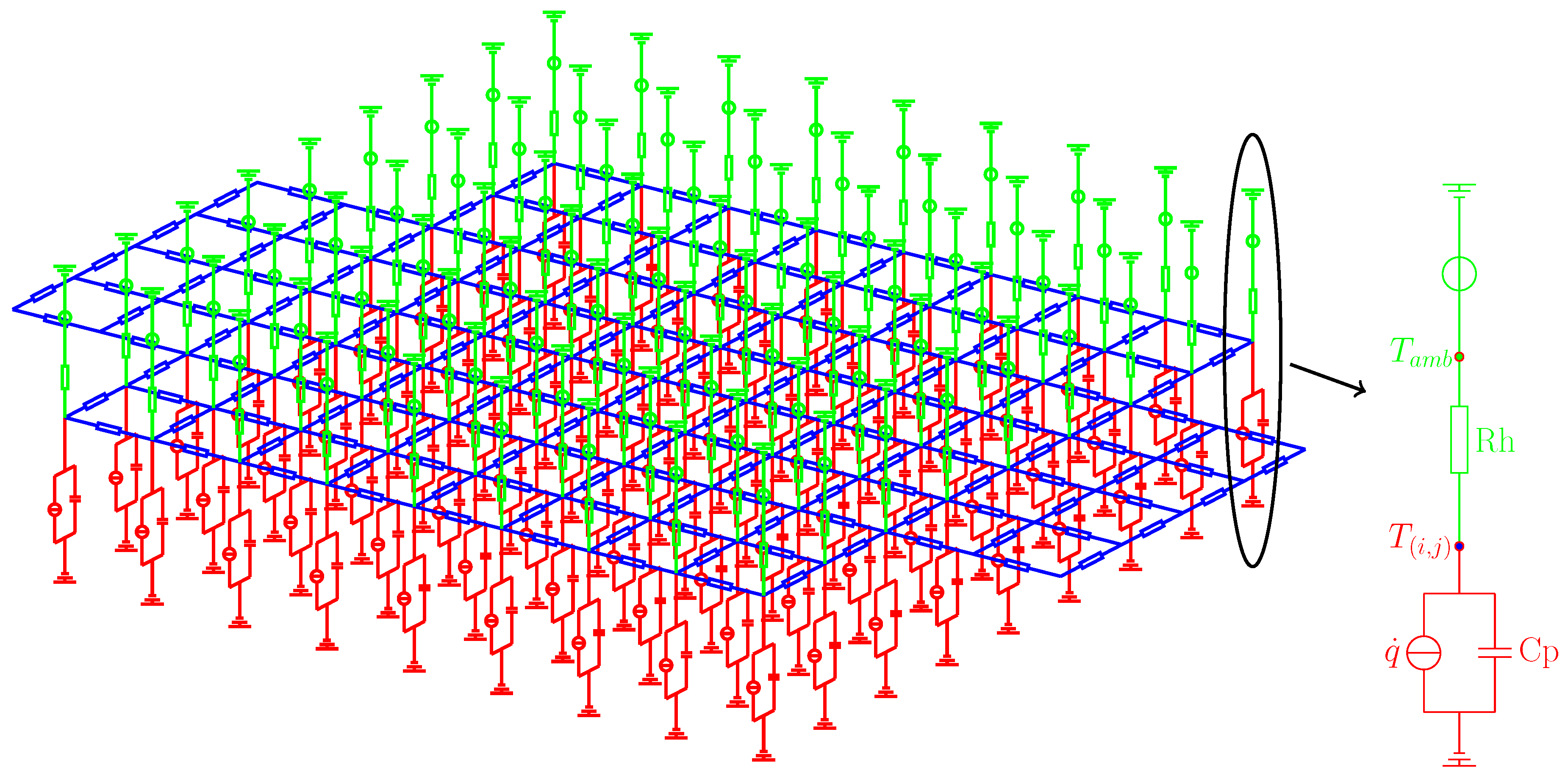
3.2. Thermal Model

The schematic of the thermal part in DPECM is shown in Figure 10. Each sub-model consists of a parallel branch of the current source and capacitor, a resistor and a voltage reference [28]. The current source represents the heat generation source. The capacitor represents the heat capacitance of the sub-model. The voltage reference provides the ambient temperature of the sub-model. The resistor represents the resistance of heat conduction and convention from the sub-model to the ambient environment. The heat conduction in the cell is modeled by the resistors between two adjacent nodes. The values of the resistors are calculated through the thermal properties of each layer using the method proposed by Chen et al. [40].

The heat generation of each sub-model is composed of irreversible and reversible heat as Equation (18):

$${\dot{q}}_{g,i}=i(e-({\phi }^{+}-{\phi }^{-}))+iT\frac{\partial e}{\partial T}$$

(18)

where ${\dot{q}}_{g,i}$ is the heat generation rate of the i-th sub-model; T is the temperature of the sub-model.

Assume that the number of thermal nodes in Figure 10 is M. As the positive and negative tabs do not have connected sub-models, where the generated heat of those nodes are set to zero, so the heat generation rate of all of the sub-models could be described as:

$$\dot{{\mathbf{Q}}_{\mathbf{g}}}={\left[\begin{array}{ccc}\underset{M-N}{\underbrace{\begin{array}{cccc}0& 0& \cdots & 0\end{array}}}& \underset{2N-M}{\underbrace{\begin{array}{cccc}{\dot{q}}_{g,1}& {\dot{q}}_{g,2}& \cdots & {\dot{q}}_{g,2N-M}\end{array}}}& \underset{M-N}{\underbrace{\begin{array}{cccc}0& 0& \cdots & 0\end{array}}}\end{array}\right]}^{\prime }$$

(19)

The heat conducted from other nodes could be calculated as:

$$\dot{{\mathbf{Q}}_{\mathbf{c}}}={\mathbf{A}}_t\mathbf{T}$$

(20)

where $\dot{{\mathbf{Q}}_{\mathbf{c}}}$ is an M-dimensional vector representing the conductive heat; $\mathbf{T}$ is an M-dimensional vector representing temperatures of all nodes; ${\mathbf{A}}_t$ is an $M\times M$ matrix representing the thermal connectivities of nodes in the thermal model, which is defined as:

$${\mathbf{A}}_T=\left[\begin{array}{cccc}-{\displaystyle \sum _{i=1}^{M,i\ne 1}}{f}_c^T(1,i)& f_c^T(1,2)& \cdots & f_c^T(1,M)\\ f_c^T(2,1)& -{\displaystyle \sum _{i=1}^{M,i\ne 2}}{f}_c^T(1,i)& \cdots & f_c^T(2,M)\\ ⋮& ⋮& \ddots & ⋮\\ f_c^T(M,1)& f_c^T(M,2)& \cdots & -{\displaystyle \sum _{i=1}^{M,i\ne M}}{f}_c^T(M,i)\end{array}\right]$$

where $f_c^T(a,b)(a,b\in 1,2,...,M\mathrm{and}a\ne b)$ is the connectivity function of the nodes in the thermal model.

The heat generation rate of the i-th node in the positive foil and tab is:

$${\dot{q}}_i^{+}=\sum _{j=1}^N{f}_c^{+}(i,j){({\phi }_i-{\phi }_j)}^2/\left(2r_{+}\right)$$

(21)

Therefore, the heat generation rate of all of the nodes on the positive foil and tab is:

$${\dot{\mathbf{Q}}}_{+}={\left[\begin{array}{cc}\underset{N}{\underbrace{\begin{array}{cccc}{\dot{q}}_1^{+}& {\dot{q}}_2^{+}& \cdots & {\dot{q}}_M^{+}\end{array}}}& \underset{M-N}{\underbrace{\begin{array}{cccc}0& 0& \cdots & 0\end{array}}}\end{array}\right]}^{\prime }$$

(22)

Similarly, the heat generation rate of all of the nodes on the negative foil and tab is:

$${\dot{\mathbf{Q}}}_{-}={\left[\begin{array}{cc}\underset{M-N}{\underbrace{\begin{array}{cccc}0& 0& \cdots & 0\end{array}}}& \underset{N}{\underbrace{\begin{array}{cccc}{\dot{q}}_1^{-}& {\dot{q}}_2^{-}& \cdots & {\dot{q}}_M^{-}\end{array}}}\end{array}\right]}^{\prime }$$

(23)

The temperatures of all of the nodes can be calculated as Equation (24):

$$\mathbf{T}={\mathbf{T}}_0+\Delta t(\dot{{\mathbf{Q}}_{+}}+\dot{{\mathbf{Q}}_{-}}+\dot{{\mathbf{Q}}_{\mathbf{c}}}+\dot{{\mathbf{Q}}_{\mathbf{g}}})/\left(mC\right)$$

(24)

where ${\mathbf{T}}_0$ is the initial temperature vector; $\Delta t$ is the step time; m is the equivalent mass of the battery block corresponding to the sub-model; C is the equivalent specific heat capacity of the battery.

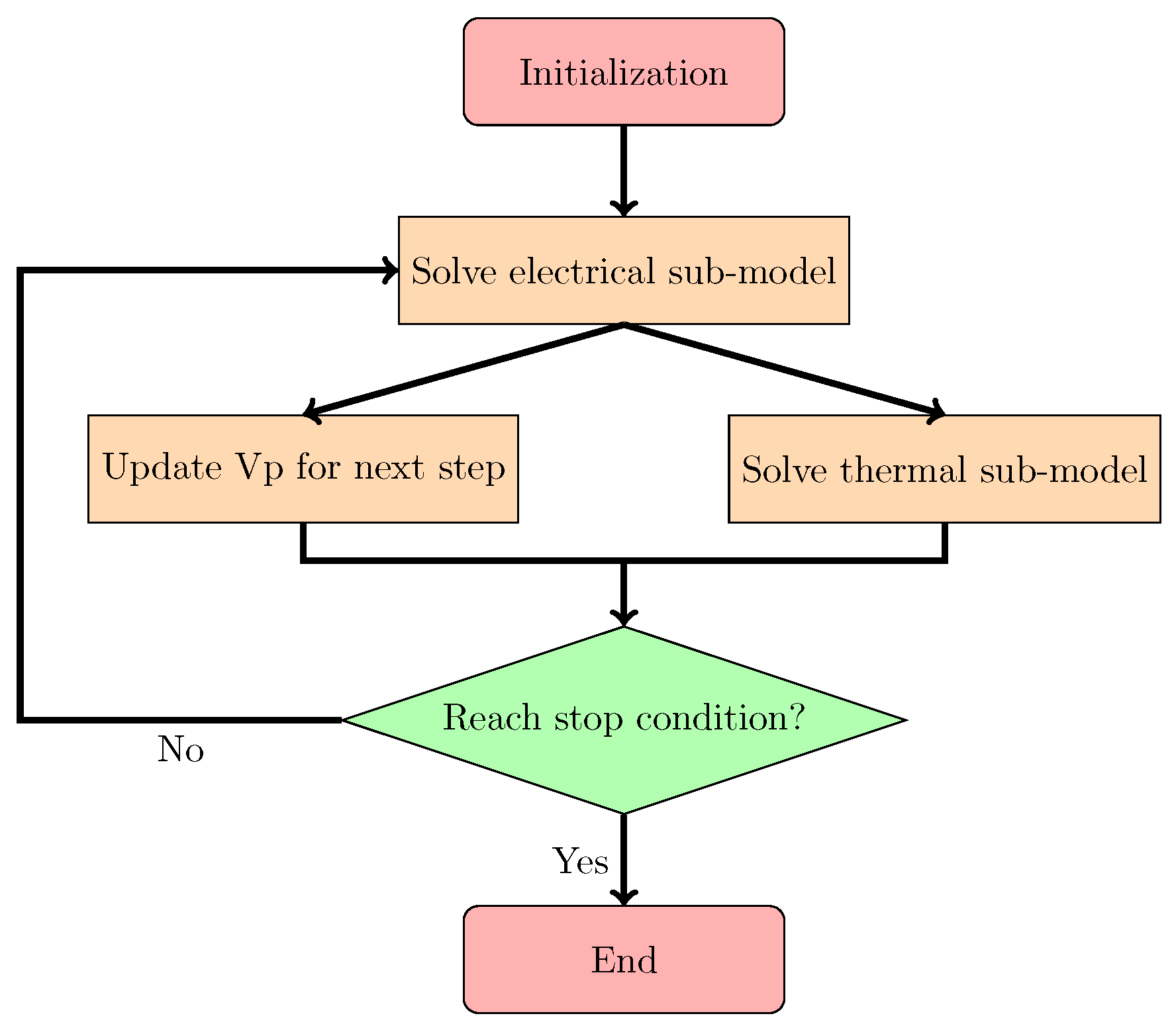
3.3. Solution

The above proposed model is built and solved using MATLAB language (M-code). The solution of the potential and current density of each sub-model can be obtained by Equations (11) and (15). The advantage of this method is that the variables in the electrical part are coupled directly. Then, the ${\mathbf{V}}_p$ of the next step is predicted. At the same time, the outputs of the electrical model are used to calculate the heat generation rate, so the thermal part of the model can be solved. The flow chart of the solving method is shown in Figure 11.

4. Results and Discussion

The simulated and experimental temperatures at the cell center ($T(2,2)$) and positive side center ($T(1,2)$) during 1C, 2C and 3C discharge are shown in Figure 12. The simulated temperature conforms with the experimental data very well, and the simulated temperature error is less than 1 °C. The accurate temperature results indicate that the proposed model has the capability of predicting internal situations in the cell.

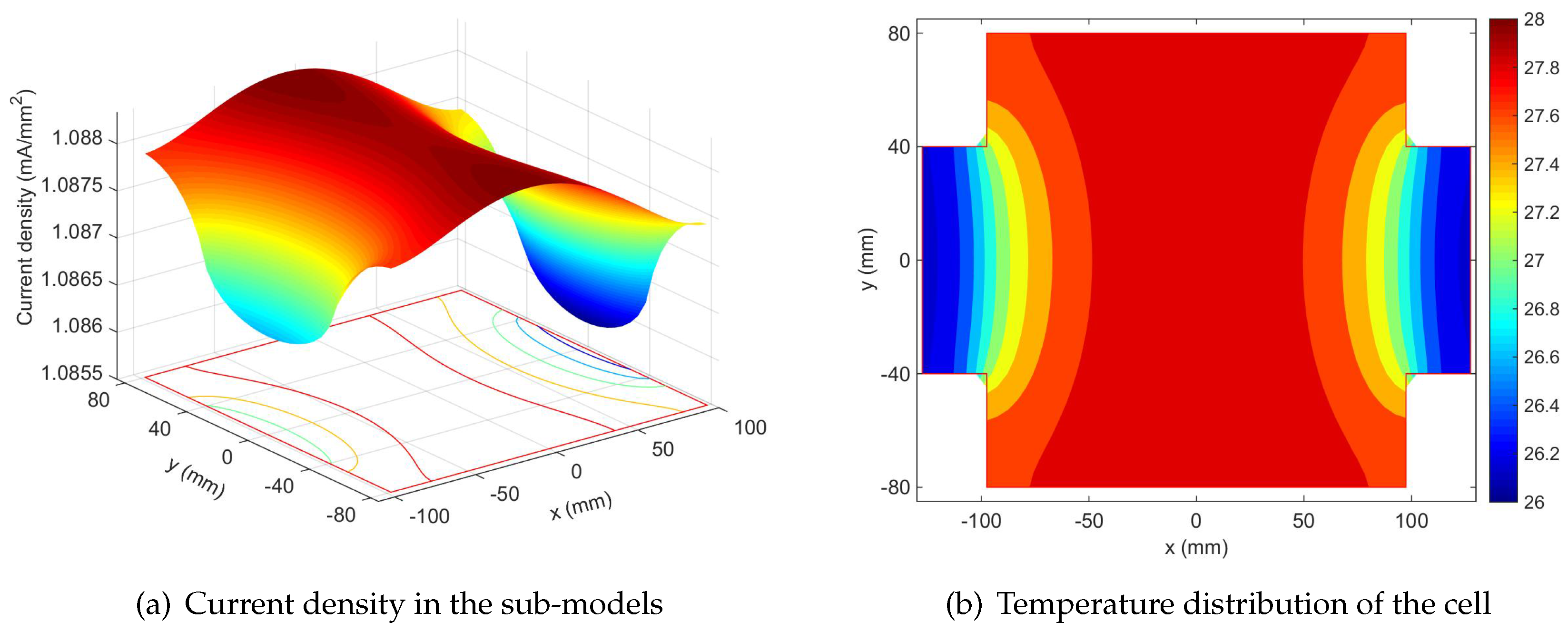
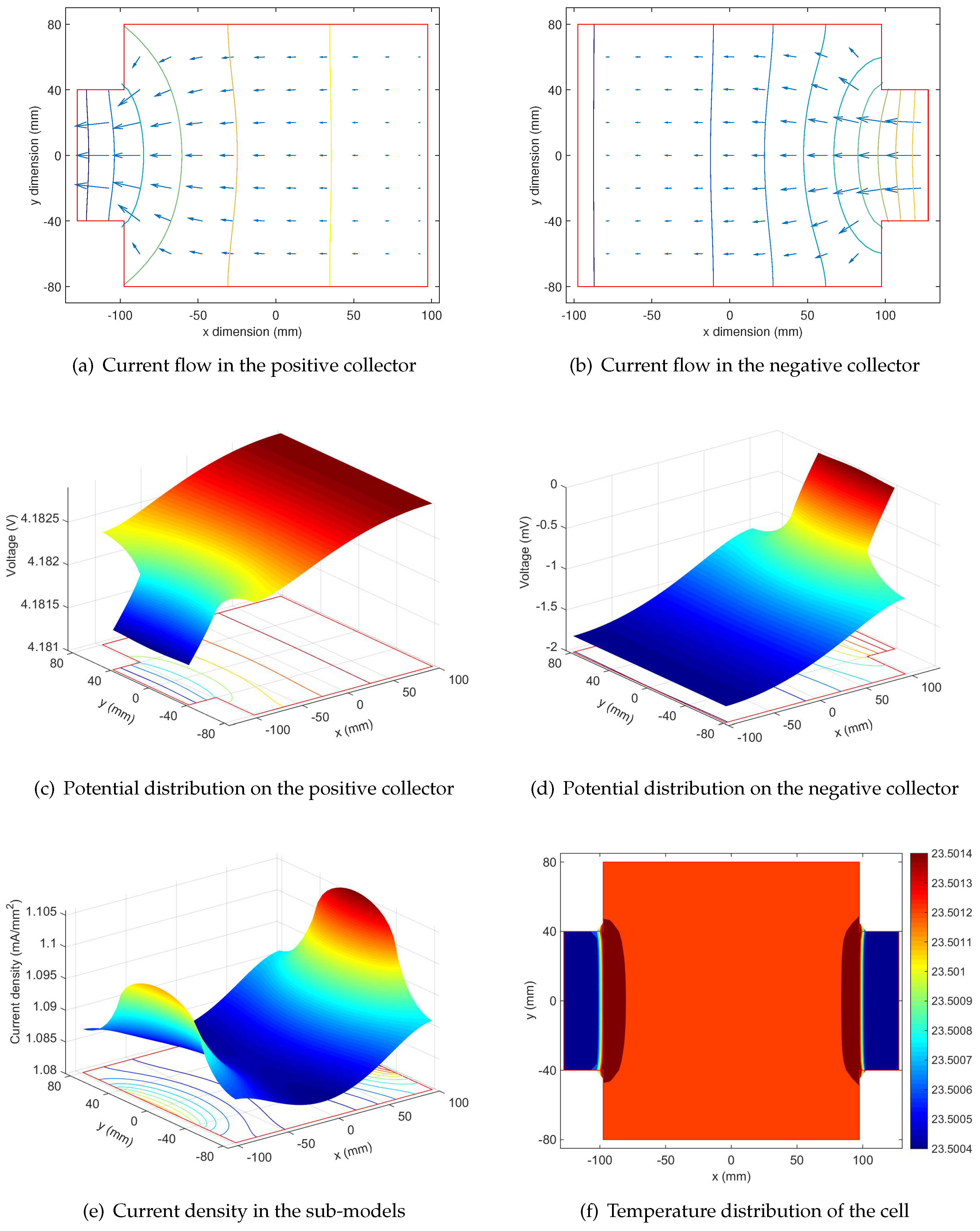
4.1. Non-Uniformity Distribution at the Initial State

During discharge, according to the structure shown in Figure 9, the current from sub-models flows through the positive foil and then is collected at the positive tab end. After the current passes the external circuit and comes back to the negative tab end, it is allocated to sub-models through the negative foil. At the beginning of battery charge/discharge, SOC and temperature are uniform in all sub-models since the battery is rested to steady state, but the current distribution becomes non-uniform when the current flows to relatively narrow tabs. Figure 13a,b shows the current density in the positive and negative current collectors, respectively. The direction of arrows represents the current direction, and the length of arrows represents the magnitude of the current flow. Therefore, the current close to tabs is larger than that in the opposite side. Figure 13c,d shows the potential of the positive and negative collectors, respectively. Since the thickness of each foil is uniform, large potential drops are produced close to tabs because of larger current flow in those areas. Figure 13e shows the current density in sub-models. The potential differences between two end nodes (${\phi }^{+}-{\phi }^{-}$) of sub-models close to tabs are smaller than that of the central part. At the same time, the polarization voltages of all of the sub-models are zero, and the equivalent potentials of all of the sub-models are equal at the beginning of the discharge. Therefore, the current flows through the sub-models, decided by Equation (2), close to tabs are higher at the beginning of the discharge process. The temperature close to tabs, shown in Figure 13f, is higher due to higher current density in foils and sub-models.

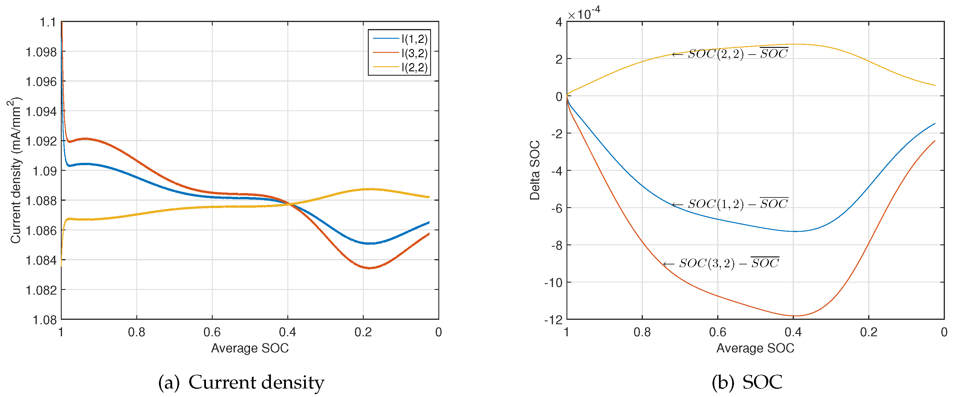
4.2. Non-Uniformity Evolution During Discharge

The non-uniformity becomes more complex after the initial state. It changes with the current profile and ambient temperature. The distribution of the current density and temperature in the sub-models could change dramatically, which sometimes even turns into an inverse distribution compared with the initial state.

The distributions of current flowing through sub-models and temperature at the end of the 1C discharge are displayed in Figure 14. Figure 14a indicates that the current density close to tabs becomes smaller than those at the cell center, which is inverse compared to the situation at the initial state, as shown in Figure 13e. This is associated with the non-uniform current accumulation and potential change in the sub-models. The current of the sub-model is calculated by $(e-({\phi }^{+}-{\phi }^{-})-u_p)/r_{\Omega }$, so the current is decided by both the potential (e) and the voltage difference between positive and negative foils (${\phi }^{+}-{\phi }^{-}$). The voltage difference between positive and negative foils close to tabs is always smaller than that at the cell center during discharge because of the existence of foil resistance and the current flow direction. While the accumulation of larger current in the sub-model causes lower local SOC during the discharge process, the local SOC of the sub-models close to tabs becomes lower than that at the cell center. Therefore, the potential difference of sub-models close to tabs and the cell center increases gradually. The influence of the potential difference becomes stronger along with the accumulation of non-uniform current distribution and finally dominates the current of the sub-models, which inverses the current density distribution. Figure 14b indicates that the temperature at the cell center becomes the highest, which is mainly due to the poor heat dissipation at the center.

To further illustrate the evolution of internal non-uniformity during discharge, three points (P(1,2), P(2,2) and P(3,2) in Figure 1) are selected to be analysis points. The current density and local SOC at those three points are calculated and presented in Figure 15. Figure 15a indicates that the difference of the local current density declines at the beginning of the discharge. The current at P(3,2) is the largest, and the current at P(2,2) is the smallest. The current becomes uniform at around SOC = 0.38. After the current crosses the point at SOC = 0.38, the current difference rises again, leading to the current at P(2,2) being the largest. The current difference decreases again after SOC around 0.2.

The current non-uniformity will cause a local SOC difference of each sub-model as shown in Figure 15b. The local SOC difference increases before the current cross point and decreases later, which can be explained by its definition. The SOC, defined as:

$$\mathrm{SOC}={\mathrm{SOC}}_0+\frac{\int idt}{3600C}$$

(25)

is decided by the initial state and current flow through the sub-model. The local SOC difference reaches the maximum value at the current cross point and then is eliminated by the inversed current density distribution. The appearance of the current cross point is caused by the relatively flat characteristics of $\mathrm{d}e/\mathrm{d}\mathrm{SOC}$ and $\mathrm{d}r/\mathrm{d}\mathrm{SOC}$ between $0.8>\mathrm{SOC}>0.2$, as shown in Figure 16. The effects of resistance in foils are counteracted by the parameter difference caused by the local SOC difference at the current cross point. After the current cross point in Figure 15a, the increase of the $\mathrm{d}e/\mathrm{d}\mathrm{SOC}$ difference becomes larger and dominates the current distribution, which enlarges the difference of the current density. It is worth noting that the direction of currents in sub-models remains the same, while the shape of the current density distribution changes from the bowl-shaped distribution to the peak-shaped distribution. The rapid increase in cell impedance after $\mathrm{SOC}<0.2$ makes the difference in current density decrease again.

4.3. Limitation of Technique

As mentioned in Section 1, the distributions of internal potential, current density or SOC can hardly be measured directly without changing the geometry and characteristics of the commercial lithium ion battery. Though the proposed model has the capability of predicting internal temperature, current density and potential, only the distributions of internal temperatures can be measured even using a customized battery. Therefore, only the internal temperatures predicted by the proposed model are validated at the present stage.

5. Conclusions

In this paper, a DPECM model consisting of a directly-coupled electrical model and a thermal model for a lithium ion battery is proposed. The model is simpler than the 3D electrical-chemical thermal model, and the parameters are easier to obtain, which is similar to the lumped ECM model. However, the proposed model has the capability of simulating the internal distribution of the current density, potential and temperature inside a cell. The model is validated by comparing the simulated temperature with measured results at test points in a customized cell that is embedded with nine T-type thermocouples. The simulated temperature error is less than 1 °C, indicating that the model can be applied to predict the internal characteristics of the battery. Summarizing the simulation results, the following conclusions can be obtained:

• The initial non-uniformity of current density inside a 35-Ah NCM pouch cell is caused by the electrode foil resistance and relatively narrow tab.
• The current flow through the sub-models close to tabs is higher than that at the center at the beginning of discharge, because the potential drops in positive and negative foils.
• A current cross point exists during the constant discharge process. The local SOC difference increases with the reduction of the average SOC until the average SOC arrives at that point and then decreases until the average SOC arrives at zero.
• The current flow through the sub-models close to tabs becomes lower than that at the center at the end of discharge due to the accumulation of the local SOC difference, rapid OCV drop and rapid resistance increase.

References

- Doyle, M.; Fuller, T.F.; Newman, J. Modeling of galvanostatic charge and discharge of the lithium/polymer/insertion cell. J. Electrochem. Soc. 1993, 140, 1526–1533. [Google Scholar] [CrossRef]
- Luo, W.; Lyu, C.; Wang, L.; Zhang, L. A new extension of physics-based single particle model for higher charge–discharge rates. J. Power Sources 2013, 241, 295–310. [Google Scholar] [CrossRef]
- Kim, G.H.; Smith, K.; Lee, K.J.; Santhanagopalan, S.; Pesaran, A. Multi-domain modeling of lithium-ion batteries encompassing multi-physics in varied length scales. J. Electrochem. Soc. 2011, 158, A955–A969. [Google Scholar] [CrossRef]
- Lee, K.J.; Smith, K.; Pesaran, A.; Kim, G.H. Three dimensional thermal-, electrical-, and electrochemical-coupled model for cylindrical wound large format lithium-ion batteries. J. Power Sources 2013, 241, 20–32. [Google Scholar] [CrossRef]
- Huo, W.; He, H.; Sun, F. Electrochemical–thermal modeling for a ternary lithium ion battery during discharging and driving cycle testing. RSC Adv. 2015, 5, 57599–57607. [Google Scholar] [CrossRef]
- Mazumder, S.; Lu, J. Faster-Than-Real-Time Simulation of Lithium Ion Batteries with Full Spatial and Temporal Resolution. Int. J. Electrochem. 2013, 2013. [Google Scholar] [CrossRef] [PubMed]
- Pals, C.R.; Newman, J. Thermal modeling of the lithium/polymer battery I. Discharge behavior of a single cell. J. Electrochem. Soc. 1995, 142, 3274–3281. [Google Scholar] [CrossRef]
- Anwar, S.; Zou, C.; Manzie, C. Distributed thermal-electrochemical modeling of a lithium-ion battery to study the effect of high charging rates. IFAC Proc. Vol. 2014, 47, 6258–6263. [Google Scholar] [CrossRef]
- Kwon, K.H.; Shin, C.B.; Kang, T.H.; Kim, C.S. A two-dimensional modeling of a lithium-polymer battery. J. Power Sources 2006, 163, 151–157. [Google Scholar] [CrossRef]
- Kim, U.S.; Shin, C.B.; Kim, C.S. Effect of electrode configuration on the thermal behavior of a lithium-polymer battery. J. Power Sources 2008, 180, 909–916. [Google Scholar] [CrossRef]
- Kim, U.S.; Shin, C.B.; Kim, C.S. Modeling for the scale-up of a lithium-ion polymer battery. J. Power Sources 2009, 189, 841–846. [Google Scholar] [CrossRef]
- Kohneh, M.M.M.; Samadani, E.; Farhad, S.; Fraser, R.; Fowler, M. Three-Dimensional Electrochemical Analysis of a Graphite/LiFePO4 Li-Ion Cell to Improve Its Durability; SAE International: Warrendale, PA, USA, April 2015. [Google Scholar]
- Liu, B.; Yin, S.; Xu, J. Integrated computation model of lithium-ion battery subject to nail penetration. Appl. Energy 2016, 183, 278–289. [Google Scholar] [CrossRef]
- Samba, A. Battery Electrical Vehicles-Analysis of Thermal Modelling and Thermal Management. Ph.D. Thesis, LUSAC (Laboratoire Universitaire des Sciences Appliquées de Cherbourg), Université de caen Basse Normandie; MOBI (the Mobility, Logistics and Automotive Technology Research Centre), Vrije Universiteit Brussel, Brussels, Belgium, 2015. [Google Scholar]
- Mastali, M.; Samadani, E.; Farhad, S.; Fraser, R.; Fowler, M. Three-dimensional Multi-Particle Electrochemical Model of LiFePO4 Cells based on a Resistor Network Methodology. Electrochim. Acta 2016, 190, 574–587. [Google Scholar] [CrossRef]
- Tong, S.; Klein, M.P.; Park, J.W. Comprehensive Battery Equivalent Circuit Based Model for Battery Management Application. In Proceedings of the ASME 2013 Dynamic Systems and Control Conference, American Society of Mechanical Engineers, Stanford, CA, USA, 21–23 October 2013. V001T05A005.
- Sun, F.; Xiong, R.; He, H. A systematic state-of-charge estimation framework for multi-cell battery pack in electric vehicles using bias correction technique. Appl. Energy 2016, 162, 1399–1409. [Google Scholar] [CrossRef]
- Yazdanpour, M.; Taheri, P.; Mansouri, A.; Schweitzer, B. A circuit-based approach for electro-thermal modeling of lithium-ion batteries. In Proceedings of the 2016 32nd Thermal Measurement, Modeling & Management Symposium (SEMI-THERM), San Jose, CA, USA, 14–17 March 2016.
- Knap, V.; Stroe, D.I.; Teodorescu, R.; Swierczynski, M.; Stanciu, T. Electrical circuit models for performance modeling of Lithium-Sulfur batteries. In Proceedings of the 2015 IEEE Energy Conversion Congress and Exposition (ECCE), Montreal, QC, Canada, 20–24 September 2015.
- Blanco, C.; Sanchez, L.; Gonzalez, M.; Anton, J.C.; Garcia, V.; Viera, J.C. An Equivalent Circuit Model with Variable Effective Capacity for Batteries. IEEE Trans. Veh. Technol. 2014, 63, 3592–3599. [Google Scholar] [CrossRef]
- Fok, C.W.E. Simulation of Lithium-Ion Batteries Based on Pulsed Current Characterization. Ph.D. Thesis, University of British Columbia, Vancouver, BC, Canada, 2016. [Google Scholar]
- Chen, X.K.; Sun, D. Modeling and state of charge estimation of lithium-ion battery. Adv. Manuf. 2015, 3, 202–211. [Google Scholar] [CrossRef]
- Xiong, R.; Sun, F.; Gong, X.; Gao, C. A data-driven based adaptive state of charge estimator of lithium-ion polymer battery used in electric vehicles. Appl. Energy 2014, 113, 1421–1433. [Google Scholar] [CrossRef]
- Zhang, S.; Xiong, R.; Cao, J. Battery durability and longevity based power management for plug-in hybrid electric vehicle with hybrid energy storage system. Appl. Energy 2016, 179, 316–328. [Google Scholar] [CrossRef]
- Xiong, R.; Sun, F.; Chen, Z.; He, H. A data-driven multi-scale extended Kalman filtering based parameter and state estimation approach of lithium-ion polymer battery in electric vehicles. Appl. Energy 2014, 113, 463–476. [Google Scholar] [CrossRef]
- Sun, F.; Xiong, R. A novel dual-scale cell state-of-charge estimation approach for series-connected battery pack used in electric vehicles. J. Power Sources 2015, 274, 582–594. [Google Scholar] [CrossRef]
- Lin, X.; Perez, H.E.; Siegel, J.B.; Stefanopoulou, A.G.; Li, Y.; Anderson, R.D.; Ding, Y.; Castanier, M.P. Online parameterization of lumped thermal dynamics in cylindrical lithium ion batteries for core temperature estimation and health monitoring. IEEE Trans. Control Syst. Technol. 2013, 21, 1745–1755. [Google Scholar]
- Forgez, C.; Do, D.V.; Friedrich, G.; Morcrette, M.; Delacourt, C. Thermal modeling of a cylindrical LiFePO4/graphite lithium-ion battery. J. Power Sources 2010, 195, 2961–2968. [Google Scholar] [CrossRef]
- Fleckenstein, M.; Bohlen, O.; Roscher, M.A.; Bäker, B. Current density and state of charge inhomogeneities in Li-ion battery cells with LiFePO4 as cathode material due to temperature gradients. J. Power Sources 2011, 196, 4769–4778. [Google Scholar] [CrossRef]
- Chen, D.; Jiang, J.; Wang, Z.; Duan, Y.; Zhang, Y.; Shi, W. Research on Distribution Parameters Equivalent-Circuit Model of Power Lithium-Ion Batteries. Trans. China Electrotechn. Soc. 2013, 7, 025. [Google Scholar]
- Zhang, G.; Shaffer, C.E.; Wang, C.Y.; Rahn, C.D. In-situ measurement of current distribution in a Li-Ion cell. J. Electrochem. Soc. 2013, 160, A610–A615. [Google Scholar] [CrossRef]
- Zhang, G.; Shaffer, C.E.; Wang, C.Y.; Rahn, C.D. Effects of non-uniform current distribution on energy density of Li-ion cells. J. Electrochem. Soc. 2013, 160, A2299–A2305. [Google Scholar] [CrossRef]
- Li, Z.; Zhang, J.; Wu, B.; Huang, J.; Nie, Z.; Sun, Y.; An, F.; Wu, N. Examining temporal and spatial variations of internal temperature in large-format laminated battery with embedded thermocouples. J. Power Sources 2013, 241, 536–553. [Google Scholar] [CrossRef]
- Huria, T.; Ceraolo, M.; Gazzarri, J.; Jackey, R. High fidelity electrical model with thermal dependence for characterization and simulation of high power lithium battery cells. In Proceedings of the 2012 IEEE International Electric Vehicle Conference (IEVC), Greenville, SC, USA, 4–8 March 2012.
- Ceraolo, M.; Lutzemberger, G.; Huria, T. Experimentally-determined Models for High-power Lithium Batteries; SAE International: Warrendale, PA, USA, April 2011. [Google Scholar]
- Xiao, M.; Choe, S.Y. Dynamic modeling and analysis of a pouch type LiMn2O4/Carbon high power Li-polymer battery based on electrochemical-thermal principles. J. Power Sources 2012, 218, 357–367. [Google Scholar] [CrossRef]
- Samba, A.; Omar, N.; Gualous, H.; Capron, O.; Van den Bossche, P.; Van Mierlo, J. Impact of Tab Location on Large Format Lithium-Ion Pouch Cell Based on Fully Coupled Tree-Dimensional Electrochemical-Thermal Modeling. Electrochim. Acta 2014, 147, 319–329. [Google Scholar] [CrossRef]
- Fu, R.; Xiao, M.; Choe, S.Y. Modeling, validation and analysis of mechanical stress generation and dimension changes of a pouch type high power Li-ion battery. J. Power Sources 2013, 224, 211–224. [Google Scholar] [CrossRef]
- Hu, X.; Li, S.; Peng, H. A comparative study of equivalent circuit models for Li-ion batteries. J. Power Sources 2012, 198, 359–367. [Google Scholar] [CrossRef]
- Chen, S.; Wan, C.; Wang, Y. Thermal analysis of lithium-ion batteries. J. Power Sources 2005, 140, 111–124. [Google Scholar] [CrossRef]