
Lumped Parameters Model of a Crescent Pump


Dipartimento Energia, Politecnico di Torino, 10129 Turin, Italy
*
Author to whom correspondence should be addressed.
Energies 2016, 9(11), 876; https://doi.org/10.3390/en9110876
Submission received: 16 August 2016
/
Revised: 27 September 2016
/
Accepted: 18 October 2016
/
Published: 26 October 2016
(This article belongs to the Special Issue Energy Efficiency and Controllability of Fluid Power Systems)
Abstract
:This paper presents the lumped parameters model of an internal gear crescent pump with relief valve, able to estimate the steady-state flow-pressure characteristic and the pressure ripple. The approach is based on the identification of three variable control volumes regardless of the number of gear teeth. The model has been implemented in the commercial environment LMS Amesim with the development of customized components. Specific attention has been paid to the leakage passageways, some of them affected by the deformation of the cover plate under the action of the delivery pressure. The paper reports the finite element method analysis of the cover for the evaluation of the deflection and the validation through a contactless displacement transducer. Another aspect described in this study is represented by the computational fluid dynamics analysis of the relief valve, whose results have been used for tuning the lumped parameters model. Finally, the validation of the entire model of the pump is presented in terms of steady-state flow rate and of pressure oscillations.
1. Introduction
Gear machines, despite their simple construction, are the most complex units to be studied from the kinematics point of view. These pumps/motors can be classified into two subcategories: external gear constituted by two external toothed rotors and internal gear where an externally toothed rotor drives an internally toothed driven gear. The latter category can be in turn divided in gerotor and crescent machines. External gear units are the most used type of fixed displacement pumps and consequently the most studied.
On the other hand, merits of the internal gear pumps are the compactness and the low flow pulsation, which leads to a reduction of the noise.
With reference to gerotor machines, based on the authors’ knowledge, about one hundred papers have been written in the last two decades covering all main aspects of this kind of machines. Among the others, studies on the hydraulic lumped parameters [1,2] and computational fluid dynamics (CFD) [3,4] models, on gear profiles optimization [5,6], contact between gear teeth [7] and friction [8] are just some examples.
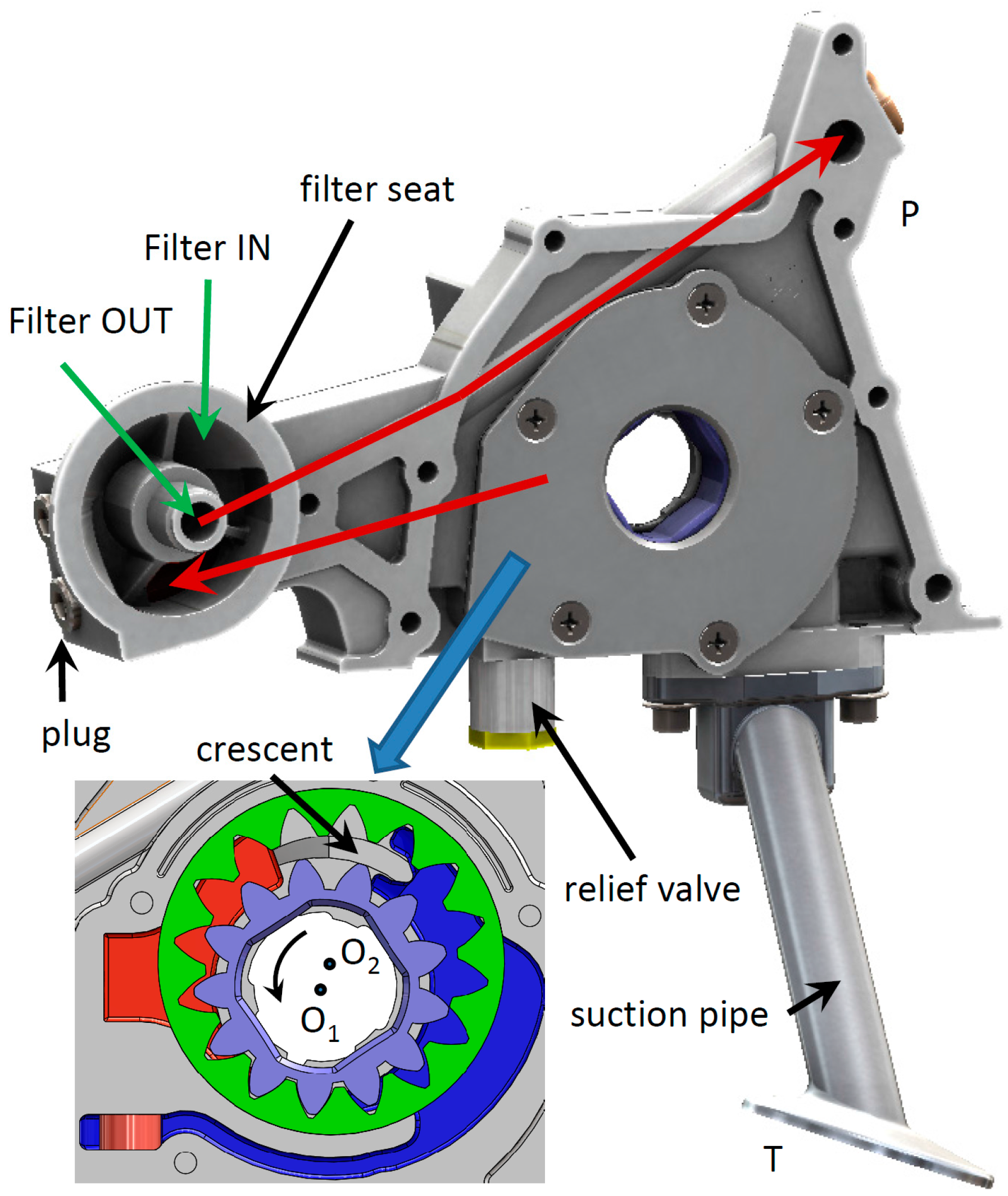
As far as the crescent machines are concerned, a view of the pump used for the present study is shown in Figure 1. The pump is used to feed the lubrication circuit of an internal combustion engine [9]. The internal gear, driven by the crankshaft, is provided with 13 teeth and rotates around the center O1. It drives the external gear with 16 teeth, which rotates around the center O2. The tooth profiles are of the involute type. Delivery and suction volumes are separated by a fixed element, called crescent. The port plate is machined directly on the housing, while on the opposite side the volumes are confined by a flat steel cover.
Due to the counterclockwise rotation of the gears, the fluid is transported along the inner and outer side of the crescent by the carry-over volumes of the driving and of the driven rotor. When the teeth mesh, the oil is delivered towards the P port. The pump is provided with an integrated pressure relief valve, whose cross section will be shown in a dedicated paragraph, which allows limiting the delivery pressure by discharging an excess flow to the suction side through a recirculation channel. The oil filter, not shown in Figure 1, is mounted directly on the pump between the gears and the outlet port P.
The studies available in the open literature on crescent pumps are quite limited and most of them are focused on kinematic aspects.
Mimmi and Pennacchi [10] compared the internal involute gear pumps and the gerotor pumps in terms of kinematic flow rate. Zhou and Song [11] determined the theoretical flow rate of a conjugated involute crescent pump under different design parameters of the gears. The same authors [12] optimized the floating plate for the axial clearance compensation of a water hydraulic internal gear pump by means of a finite element analysis. Moreover, in [13] the authors studied the conjugated straight-line profiles for internal gear pumps, with a specific focus on the non-interference condition.
Slodczyk and Stryczek [14] developed an algorithm for the design process of the main geometric parameters of the pump. The computer generation of the profiles for crescent pumps was also implemented by Fetvaci [15].
As far as the hydraulic model is concerned, in [16] Jiang et al. presented a 3D CFD of an oil pump developed in PumpLinx®. Instead Guo et al. [17] used ANSYS Fluent® for a 2D CFD model. It is out of discussion that a CFD model represents the most advanced technique for the study of a positive displacement machine. However, the huge difference in terms of computational time, some minutes or less of a lumped parameters model against several hours of a CFD code, makes the former still competitive for some types of studies.
In this paper, a lumped parameter model of a crescent pump with an integrated relief valve is presented. The main geometric features are calculated as function of the gears’ parameters. The study also includes a finite element method (FEM) for taking into account the variation of the clearances due to the deflection of the pump cover and a CFD analysis of the flow through the relief valve. The complete model has been demonstrated to be reliable to reproduce the main performance characteristics with minor tunings.
The aim of the study is the development of a quite detailed model able to predict the delivered flow rate and the pressure ripple. The former feature can be used to improve the volumetric efficiency in the design phase, in order to obtain the same flow rate with a smaller gear set, leading to a lower viscous friction and to a reduction of the absorbed power. The latter is necessary to optimize the pump in order to reduce the fluid-borne noise. Moreover, the use of the model is twofold: a tool for the optimization of the pump itself or a subcomponent to be used to analyze the interaction with a model of an entire fluid power system.
2. Mathematical Model
2.1. Control Volumes
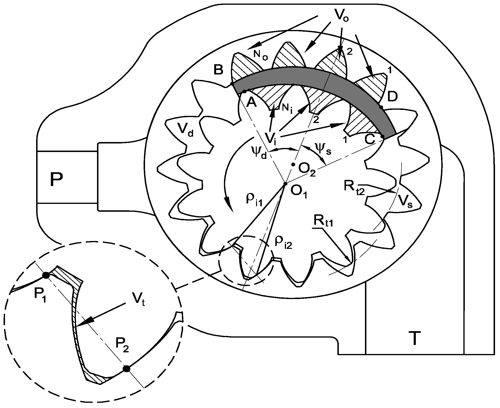
The pump is divided in control volumes (Figure 2). The approach used in the present study is to consider three variable hydraulic capacities associated with the delivery Vd, suction Vs and trapped Vt volumes, and a variable number of fixed capacities associated with the carry-over volumes of the inner Vi and of the outer Vo gear. With this method, all chambers connected to the outlet side between the points A, B and P1 are lumped together and with the delivery volume and are considered as a single entity identified by a unique value of pressure. In a similar way, the chambers connected to the inlet side between the points C, D and P2 form the suction volume. The third variable capacity, defined only for a limited angular range, is represented by the trapped volume between the points P1 and P2. In fact, for some shaft positions only one contact point between the gears separates the delivery and the suction volumes.
The number of carry-over volumes Vi and Vo is variable and ranges between Ni − 1 and Ni for the inner gear and between No − 1 and No for the outer gear. Hence, it is assumed that for each gear the volumes numbered between 1 and Ni − 1 (or No − 1) are always defined, while the last volume Ni (or No) exists only for a limited angular range. The maximum number of carry-over volumes for the driving gear Ni depends on the angular extension of the crescent:
being Δϕ the angular pitch of the inner gear. In a similar way, the number No for the driven gear is defined. To each volume, the mass conservation in isothermal conditions is applied:
being p the pressure, V the volume, Qin and Qout the ingoing and outgoing flow rates, ω and ϕ respectively the angular speed and position of the shaft and β the fluid bulk modulus.
For the evaluation of the angular derivatives of the volumes, the vector rays approach used by Mancò and Nervegna [18] for the external gear pumps and modified by Rundo [19] for internal gear machines has been implemented. The method is based on the knowledge of the length of the vector rays joining the contact points between the gears P1 and P2 with the center of rotation. These vector rays are indicated with ρi1 and ρi2 for the inner gear (see also Figure 2). In a similar way, ρo1 and ρo2 are defined for the outer gear, but in this case the center of rotation is O2 instead of O1. The expressions of the volume variations are:
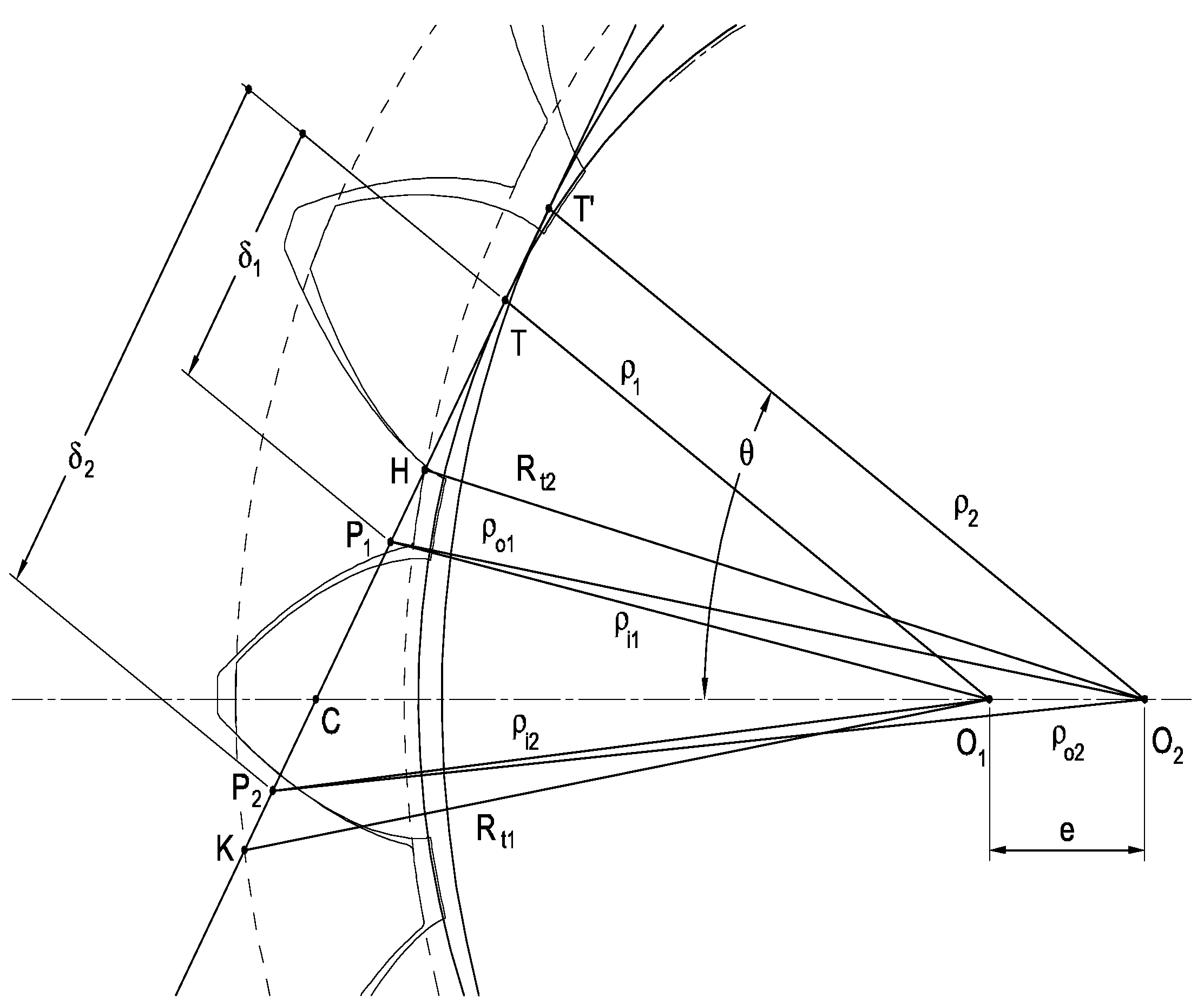
where Rt1 and Rt2 are the radii defining the tooth tips of the inner and of the outer gear respectively, τ is the transmission ratio and H the axial thickness. For the evaluation of the vectors length, an auxiliary coordinate relative to the first contact point P1, measured along the line of contact starting from the point T tangent to the base circle of the driving gear, can be defined (Figure 3).
In addition, a new angular variable νd ranging between 0 and Δϕ is defined, so that νd = 0 when the trapped volume starts to exist. The relationship between and νd is the following:
where ρ1 is the base circle of the driving gear and the constant ν01 is:
while the length of the segment can be expressed as function of the operating pressure angle θ as follows:
In a similar way, for the second contact point P2, an additional variable νs is defined, so that νs = 0 when the trapped volume ends to exist, therefore:
where:
moreover, the length of the segment is:
When the trapped volume exists, it is also possible to write:
With reference to the Figure 3 and according to the Equation (6) the square of the vector ray belonging to the driving gear relative to the contact point P1 is:
while for the driven gear the vector ray is:
If the contact point P2 is now considered, the vector rays are:
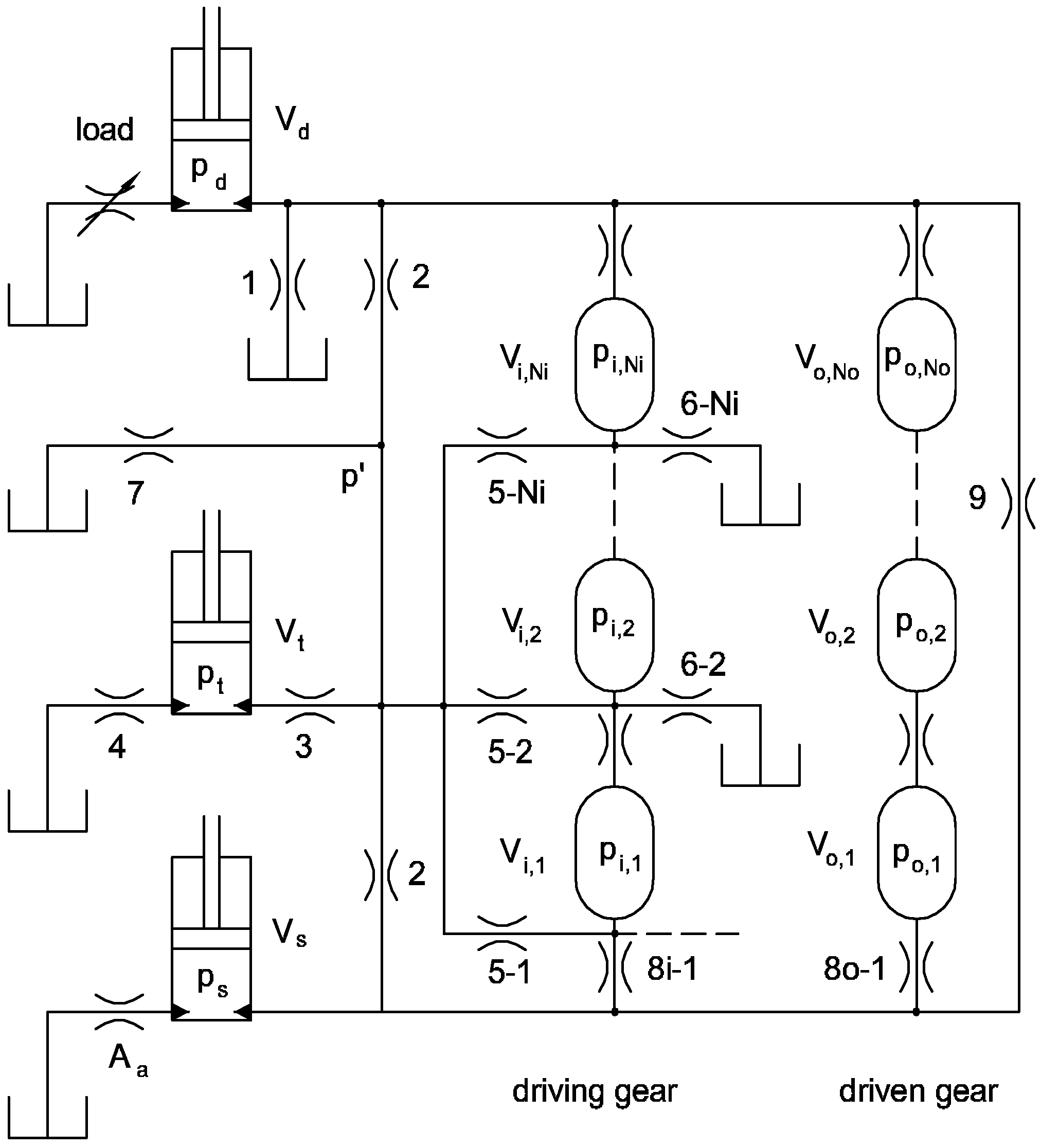
The complete hydraulic circuit of the pump is shown in Figure 4, where the variable volumes are represented, for ease of understanding, as linear actuators. These volumes, with pressure pd, pt and ps, are connected together and with the fixed carry-over capacities by gaps, represented by hydraulic orifices, and described more in details in the next paragraph.
For the fixed volumes from 1 to Ni − 1 (or No − 1) the pressure is calculated with the Equation (2) without the term due to the angular derivative. Moreover, the first volume is always connected with the suction volume. For the last capacity Ni or No and for the trapped volume the pressure is calculated with the Equation (2) only when the volume exists, otherwise the pressure is imposed to be equal to the delivery pressure. The delivery volume is connected with either the capacity Ni − 1 (No − 1) or Ni (No).
2.2. Leakages
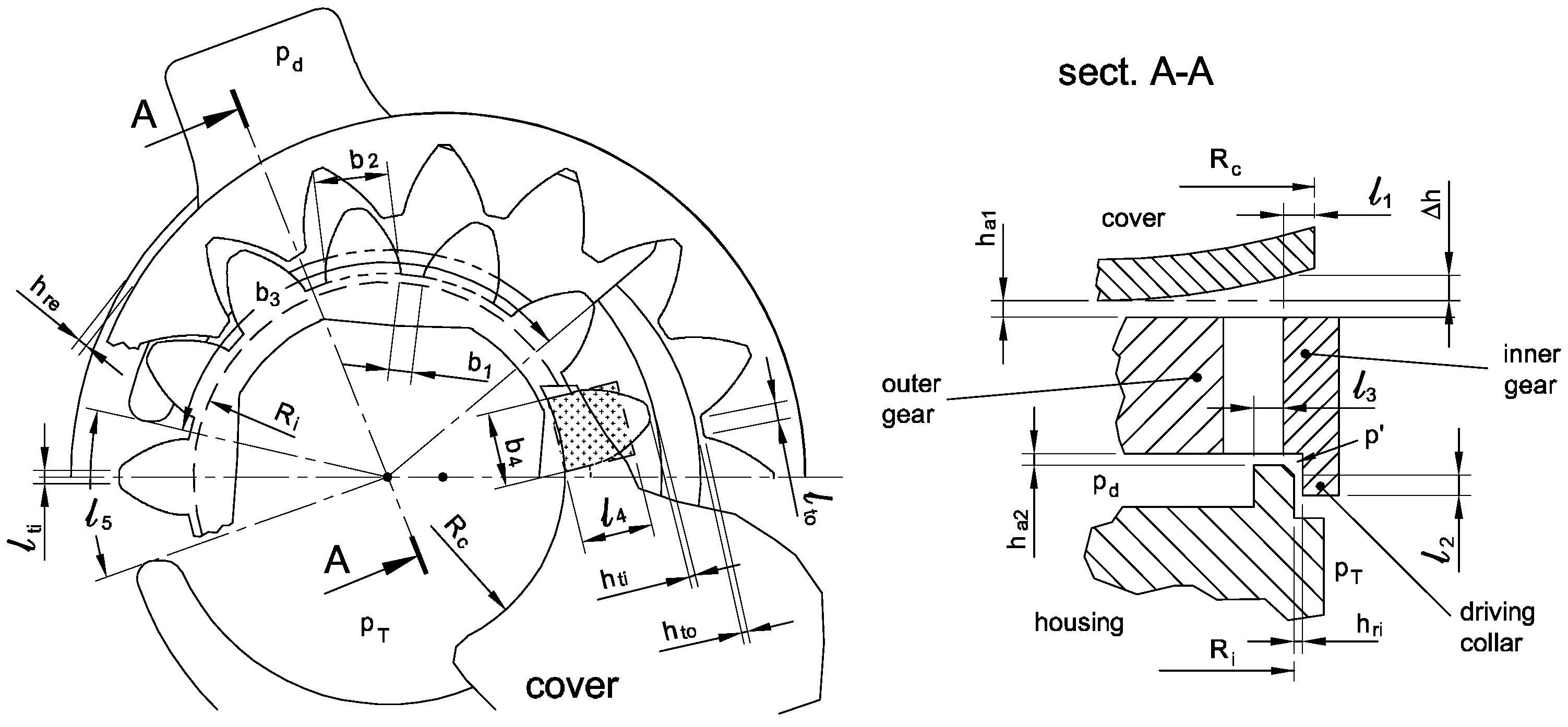
For the identification of the leakage passageways refer to Figure 5. While the formulation relative to the control volumes can be considered valid for any kind of crescent pump, some leakages depend on the specific geometry of the machine, hence the layout of the pump under study is presented. The leakages are simulated by means of fixed orifices numbered from 1 to 9 in Figure 4. The leakage due to the axial clearance between the inner gear and the casing on the cover side (orifice 1) is split into two terms. The first one is the flow Ql1a at the tooth roots through the gap formed by the overlap with length l1 and width b1 between the cover and the inner gear, while the term Ql1b due to the gap between the side of the teeth and the cover.
The first term is given by the Equation (17):
where nt is the mean number of teeth exposed to the delivery pressure, in this case five and μ is the dynamic viscosity. The axial clearance is incremented by the maximum cover deformation Δh that occurs in correspondence of the inner radius Rc, as demonstrated in the paragraph 3.
For the second term, an equivalent rectangular gap with width b4 and length l4 equal to 0.75 times the tooth height is considered. Moreover, the mean cover deformation is assumed 75% of the maximum value Δh. Hence, the flow rate is calculated with the expression (18):
Also for the axial clearance on the casing side (orifice 2), two different passageways in parallel are considered: the flow area at the tooth roots with width b1 and height ha2 and the rectangular gap between the teeth and the casing with length l3, width b2 and height ha2. The flow rates are respectively:
where p′ is the pressure in the chamfer volume, ρ the fluid density and Cd the discharge coefficient.
The same equations are used for the flow between the chamfer volume and the suction side, with the only difference that the pressure drop in this case is p′. Similar leakages also occur in the trapped volume and in the carry-over volumes. For the trapped volume, radial flow rates through the axial clearances (gaps 3 and 4 for casing and cover sides respectively) are calculated in a simplified way as follows:
For each carry-over volume of the inner gear (gaps 5 and 6), the same Equations (21) and (22) are used, with simply the pressure pi,j instead of pt, with i from 1 to Ni.
The oil leaking from the gaps 2, 3 and 5 flows through the clearance between the casing and the driving collar of the inner gear with length l2. The collar works as a journal bearing with eccentricity ratio ε and the flow rate is calculated with the Equation (23):
In order to evaluate a reasonable value for ε, an Ocvirk model was used. It is suitable to calculate the operating condition of a bearing where the ratio between the diameter and the axial length is greater than 2 (short bearing). The model is based on the hypothesis that it is possible to neglect, in the tangential direction, the flow rate due to the pressure gradient (Poiseuille flow) with respect to the flow rate due to the bearing rotation (Couette flow). In this way, it is possible to simplify the Reynolds equation for the pressure distribution in the bearing, which can be integrated analytically. For the pump under study, a value of ε around 0.95 is a good compromise for the entire speed range.
The carry-over volumes are connected one each other through the gaps hti and hto between the tooth tips and the crescent. Moreover, two additional passageways are originated by the axial clearances ha1 and ha2 on the two sides of the gears. However, these last contributions can be neglected, since the mean length of the gap b4 is quite higher than the length of the gaps on the tooth tips lti and lto.
The leakage flow between two consecutive carry-over volumes is calculated with the Equations (24) and (25) respectively for the inner and the outer gear:
where the second term represent the Couette flow due to the drag of the oil in the gap.
For the leakage due to the radial clearance between the outer gear and the casing, it was assumed that the gap is entirely recovered on one side. On the other hand, the influence of this leakage is marginal due to the high gap length; hence, a more complex formulation is not necessary. The leakage is calculated as follows:
3. FEM Model of the Cover
As already demonstrated in [20,21], for a crankshaft mounted lubricating pump the deformation of the cover plate has a significant influence. To take into account the variation of the axial gap between the gears and the housing, a finite element method (FEM) study was performed with the ANSYS package.
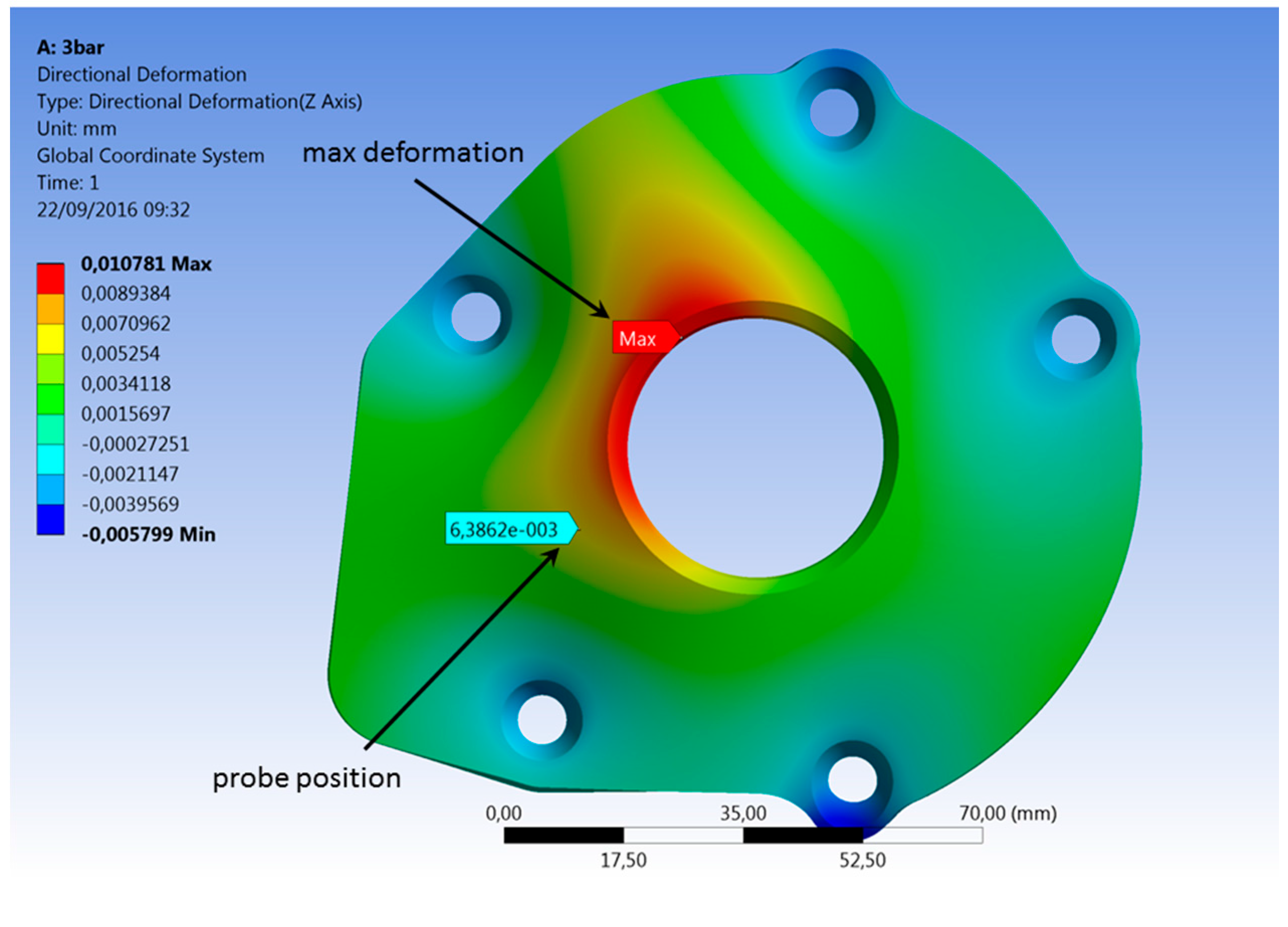
The cover was discretized with four-node shell type cells with a size of 0.7 mm, leading to about 1 million elements. The deformation of the screws was also taken into account. Two types of contacts were used in the model: a bonded type between the screws and the cover and between the screws and the casing, while a frictionless contact was applied between the cover and the casing. A uniform pressure was applied on the cover in correspondence of the region exposed to the delivery pressure. Figure 6 shows how the cover is distorted in the direction perpendicular to the frontal plane due to a delivery pressure of 3 bar. The region of maximum deformation (red) occurs in correspondence of the inner radius Rc of the cover.
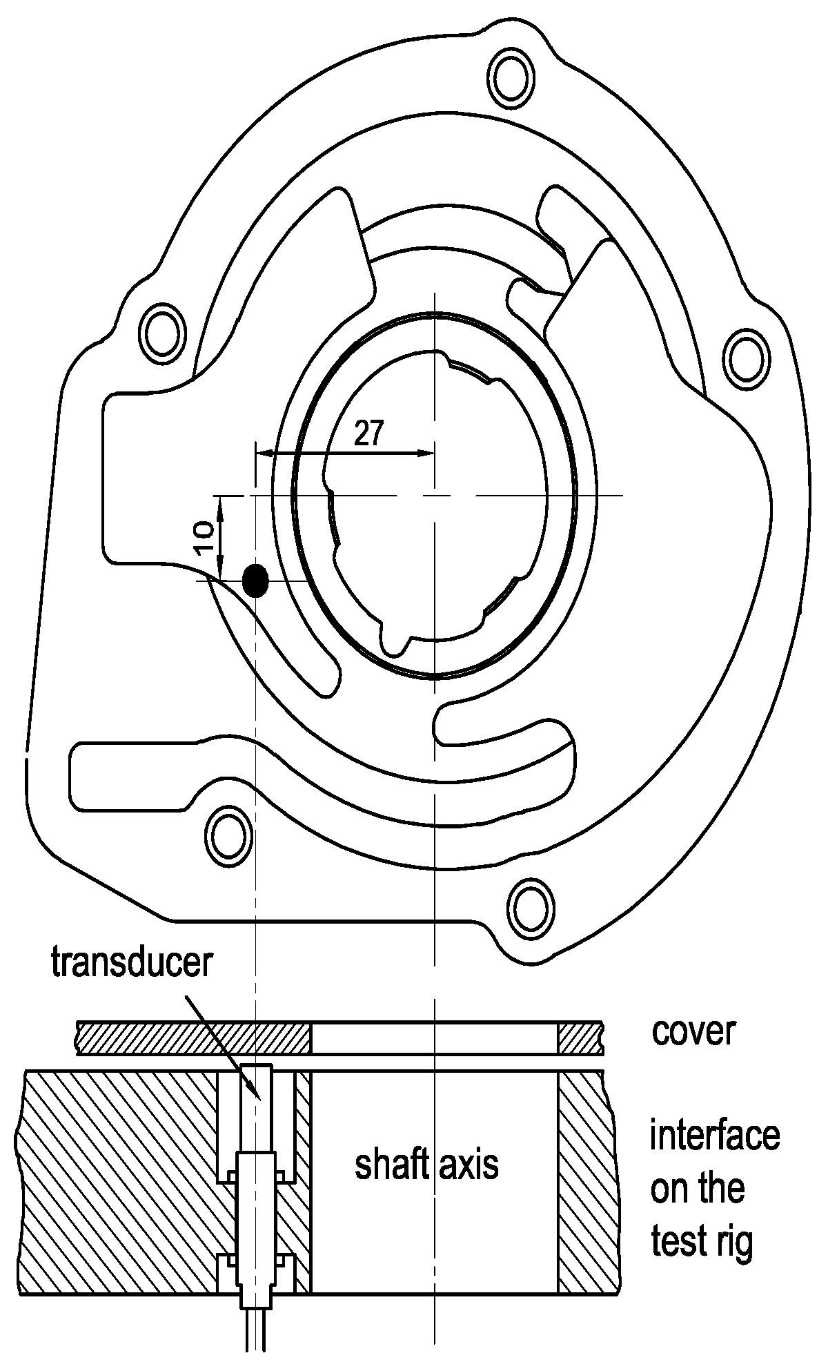
The experimental evaluation of the cover deformation was performed with a noncontact proximity transducer KAMAN KD2300-1SUM with measuring range 0–1.25 mm and resolution 0.1 μm mounted on the interface plate of the test rig as shown in Figure 7. The transducer sensed the distance from the cover in correspondence of the pump delivery volume.
Due to the high sensitivity to the temperature variation of the pump casing and of the interface block, the measurement of the absolute distance from the cover was demonstrated to be not reliable. On the other hand, a good repeatability was obtained by measuring the variation of the distance due to a fast increment of the pressure starting from a reference value (3 bar). In Table 1, the simulated variation of the cover deformation generated by a pressure increment up to 6 and 8 bar respectively is contrasted with the experimental values. In the last column the displacement of the cover in correspondence of the point of maximum deformation (see Figure 6) is also reported; these last values have been used for Δh in the Equation (17).
4. Model of the Relief Valve
4.1. Valve Description
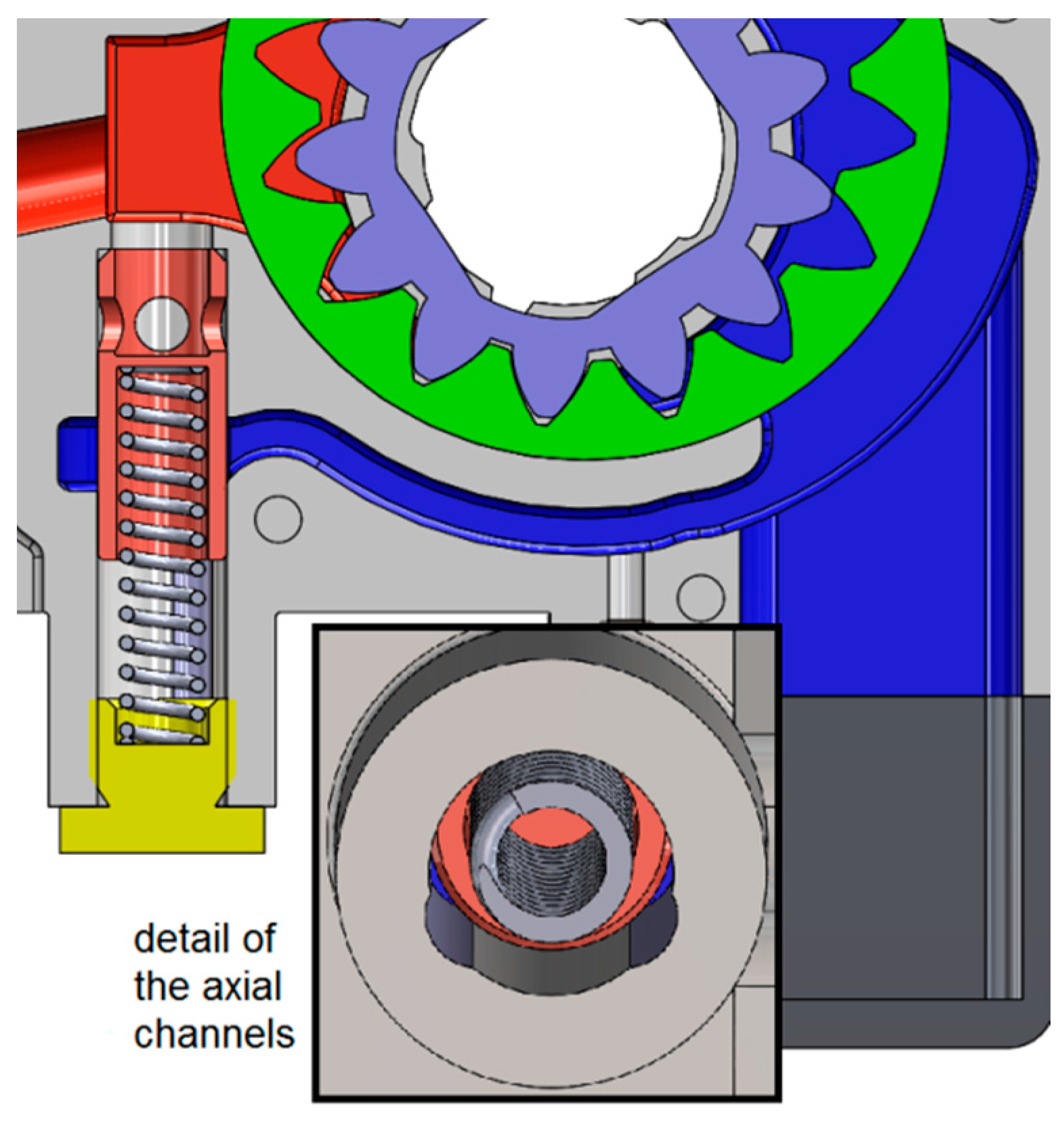
A cross section of the relief valve is shown in Figure 8. It is a normally closed valve made up of a spool with 4 holes at 90° and a spring. The delivery pressure acts on the head of the spool generating an opening force in opposition to the force exerted by the spring. When the holes are partially uncovered, the valve regulates and a flow rate recirculates from the delivery volume to the suction side.
The spring chamber is connected to the suction volume through two circular segment shaped axial channels, visible in the bottom view where the plug has been removed. In theory, these channels should impose the suction pressure in the spring chamber. However, in regulating conditions, the jet coming from the high-pressure side is able to pressurize slightly the chamber, with the generation of an additional closing force, which alters the equilibrium of the spool. This is also because the outlet of the valve is not symmetric; hence, only one of the four holes faces directly the recirculation channel. The oil, coming from the other holes, is forced to flow through a narrow passage around the spool; the consequence is the generation of a backpressure.
The effect is a modification of the steady-state flow-pressure characteristic of the valve, as also demonstrated experimentally in [1], where a similar component was tested with and without the venting of the spring chamber. Such pressurization was evaluated with the add-in FlowSimulation available in Solidworks®, moreover the CFD analysis was also used for tuning the discharge coefficient and the flow force in the lumped parameters model of the valve built in LMS Amesim with the Hydraulic Component Design (HCD) Library.
4.2. CFD Model
4.2.1. Numerical Solution Techniques
The CAD-Embedded tool FlowSimulation allows performing a flow analysis of an assembly created in Solidworks. Most of the aspects related to numerical issues are managed automatically by the software and cannot be modified by the user. However, it was verified in a previous study on fluid power valves [22] that, at least for simple geometries, good results can be obtained in the evaluation of the pressure drop, also in comparison to other CFD tools.
The governing equations are discretized using the finite volume technique. The mesh is constituted by rectangular parallelepipeds, with the exception of the boundary surfaces, where the cut cells method is applied and the mesh is polyhedral.
The spatial interpolation schemes are of the second-order, in particular upwind with limiters for the convective terms and central for the diffusive terms.
As far as the turbulence model is concerned, the Favre-averaged Navier-Stokes equations are used, with a low Reynolds k-ε Lam-Bremhorst model to close the system of equations.
A laminar/turbulent boundary layer model is used in near-wall regions. The model is based on the Two-Scale Wall Functions (2SWF) approach [23], which uses two different methods depending on the number of cells across the boundary layer. If it is greater than 5 the calculation of the laminar boundary layers is performed through the Navier-Stokes equations, while for the turbulent boundary layer by means of a modified wall function approach with the Van Driest’s velocity profile. On the contrary, if the number of cells is 5 or lower the Prandtl boundary layer equation is solved along the fluid streamlines covering the walls.
For the pressure-velocity coupling, a method based on the SIMPLE approach is implemented.
4.2.2. Model Settings
The basic mesh is constituted by cubic cells with side of 0.2 mm. In order to fill the computational domain about 1.3 million cells are required, but the minimum flow area is discretized with too few elements, leading to a poor accuracy. FlowSimulation allows defining regions where a local mesh refinement can be applied. Each refinement level consists in dividing by two the side of the original cells, hence with a 2nd level each basic element is split in 82 = 64 cells.
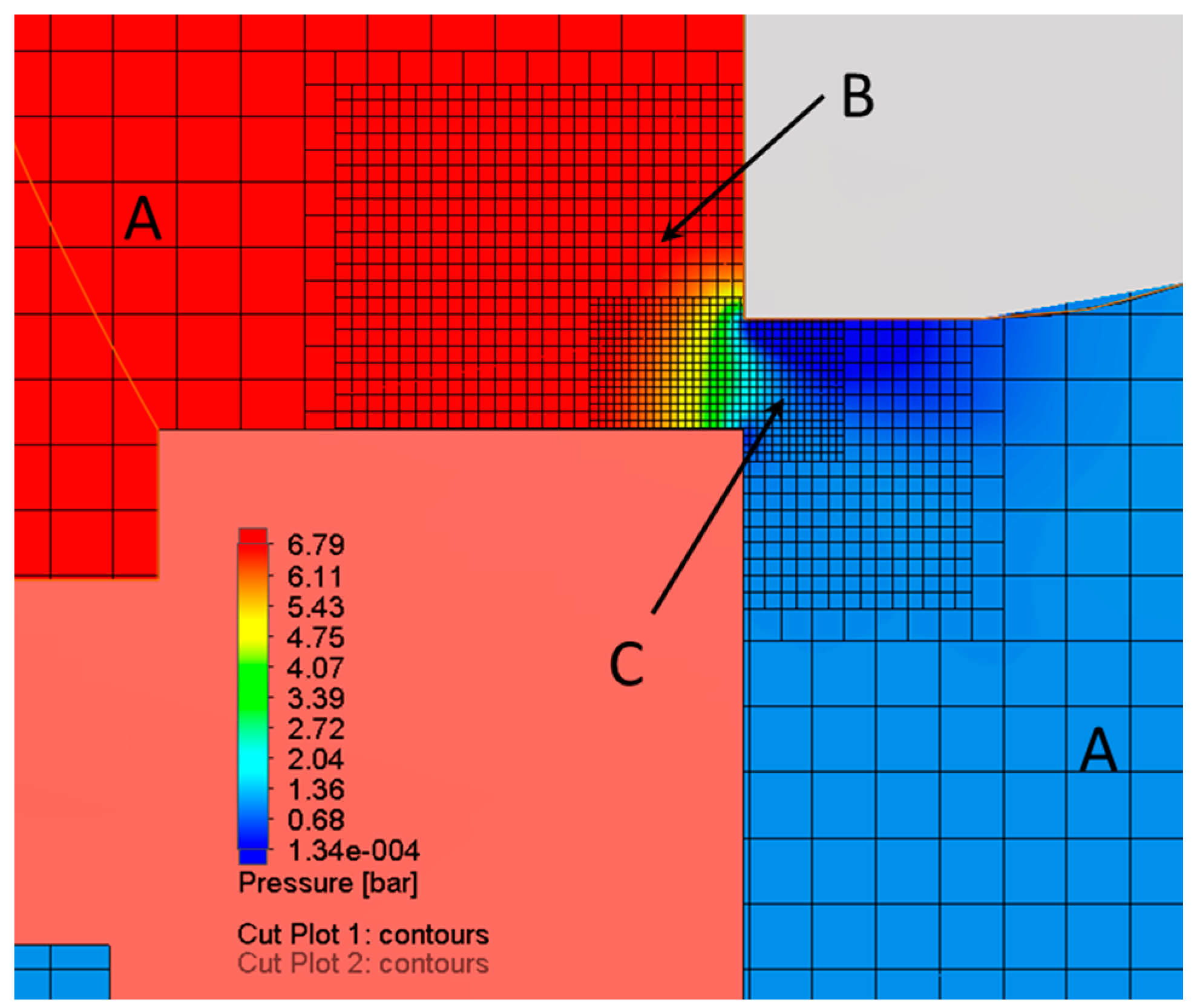
Since the pressure drop is located mainly in correspondence of the spool holes, a cell refinement was performed across the metering edges, where the pressure gradient is maximum. In Figure 9, the pressure field and the mesh refinement with a flow rate of 2 L/min and a valve underlap of 0.35 mm is shown.
Two concentric local regions B and C across the metering edge were meshed with a finer grid. In order to obtain mesh independent results, different refinement levels and combinations were analyzed for the opening of 0.35 mm. The list of the configurations is reported in Table 2, where the refinement level of the inner region C is with respect to the intermediate region B.
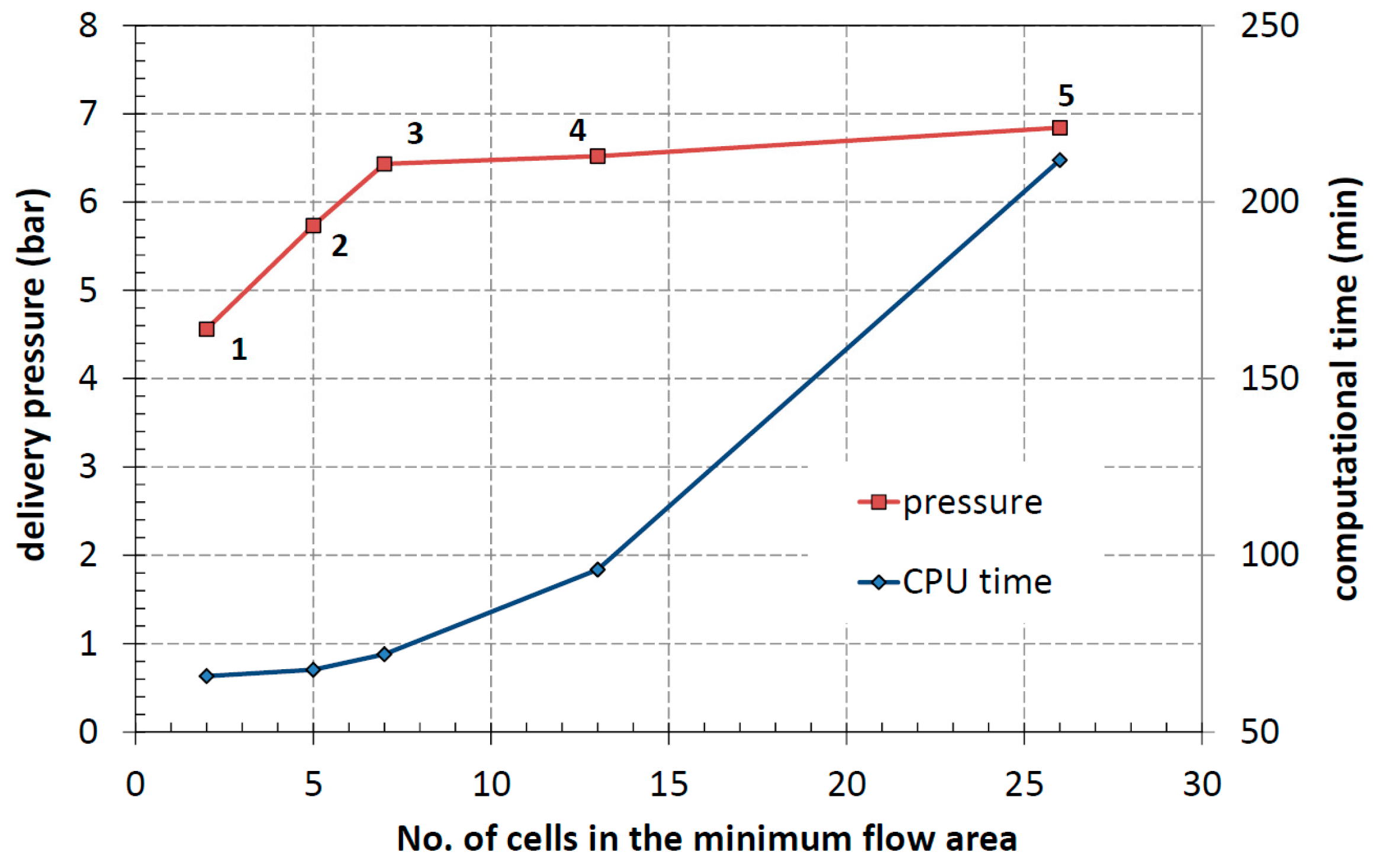
The delivery pressure simulated for different values of the number of cells (listed in Table 2 for the five configurations) into which the minimum flow area was divided are shown in Figure 10 along with the computational times on an eight-core Xeon processor at 3.4 GHz. It is also possible to notice that with about 10–15 cells a good compromise between accuracy and computational time is achieved.
Such cell density is necessary not only for a proper evaluation of the regulated pressure, but also for the correct calculation of the flow field downstream from the metering edge [24], which has an influence on the pressure in the spring chamber.
Nevertheless, it must not be excluded that a more aggressive optimization of the mesh could lead to similar results with a smaller number of cells in the regions far away from the spool or with a different extension of the regions B and C; however, such type of analysis goes beyond the aim of the present study.
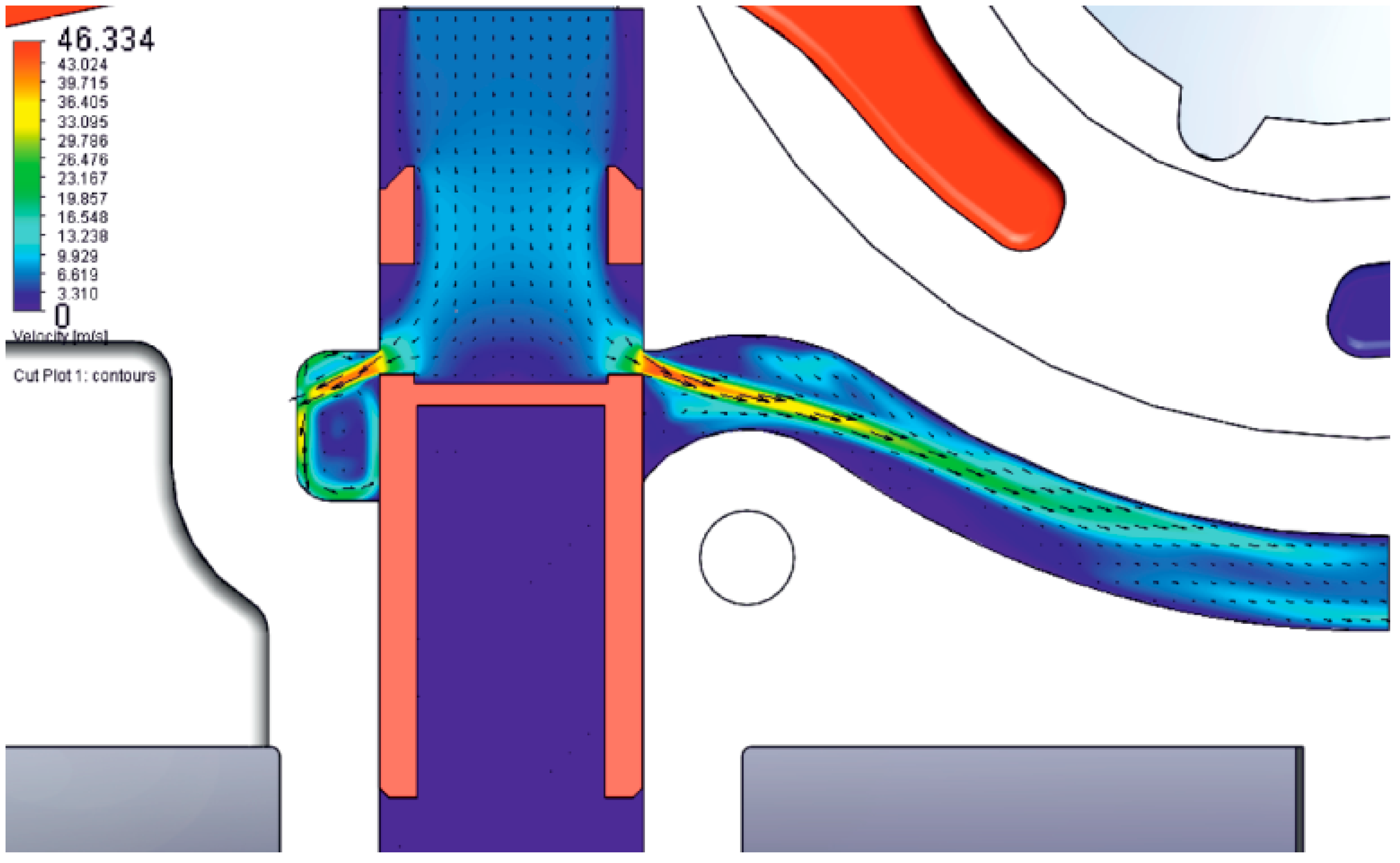
As boundary conditions, the flow rate was imposed at the inlet, while the atmospheric pressure was set at the end of the recirculation channel. Ten simulations were performed with different fixed positions of the spool, with the underlap of the holes ranging from 0.1 mm to 1.5 mm. For each position, a reasonable value of flow rate estimated with the lumped parameters model with default setting was imposed. A typical flow field in Figure 11 highlights the asymmetry of the fluid jet that cannot be reproduced by a lumped parameters model. In fact, the oil coming from the left hole is forced to flow through narrow passages before reaching the recirculation channel. The consequence is a pressure increase in the left pocked and in the spring chamber, being connected through the axial channels.
4.3. Tuning of Lumped Parameters Model
The model in LMS Amesim calculates the spool position as function of the forces due to the pressures and to the spring. Then the passage area and the flow rate are evaluated based on the position of the moveable element. With FlowSimulation for each value of the spool displacement, the following quantities were evaluated:
- the pressures at the valve inlet pd and in the spring chamber,
- the force acting on the frontal surface of the spool (opening force).
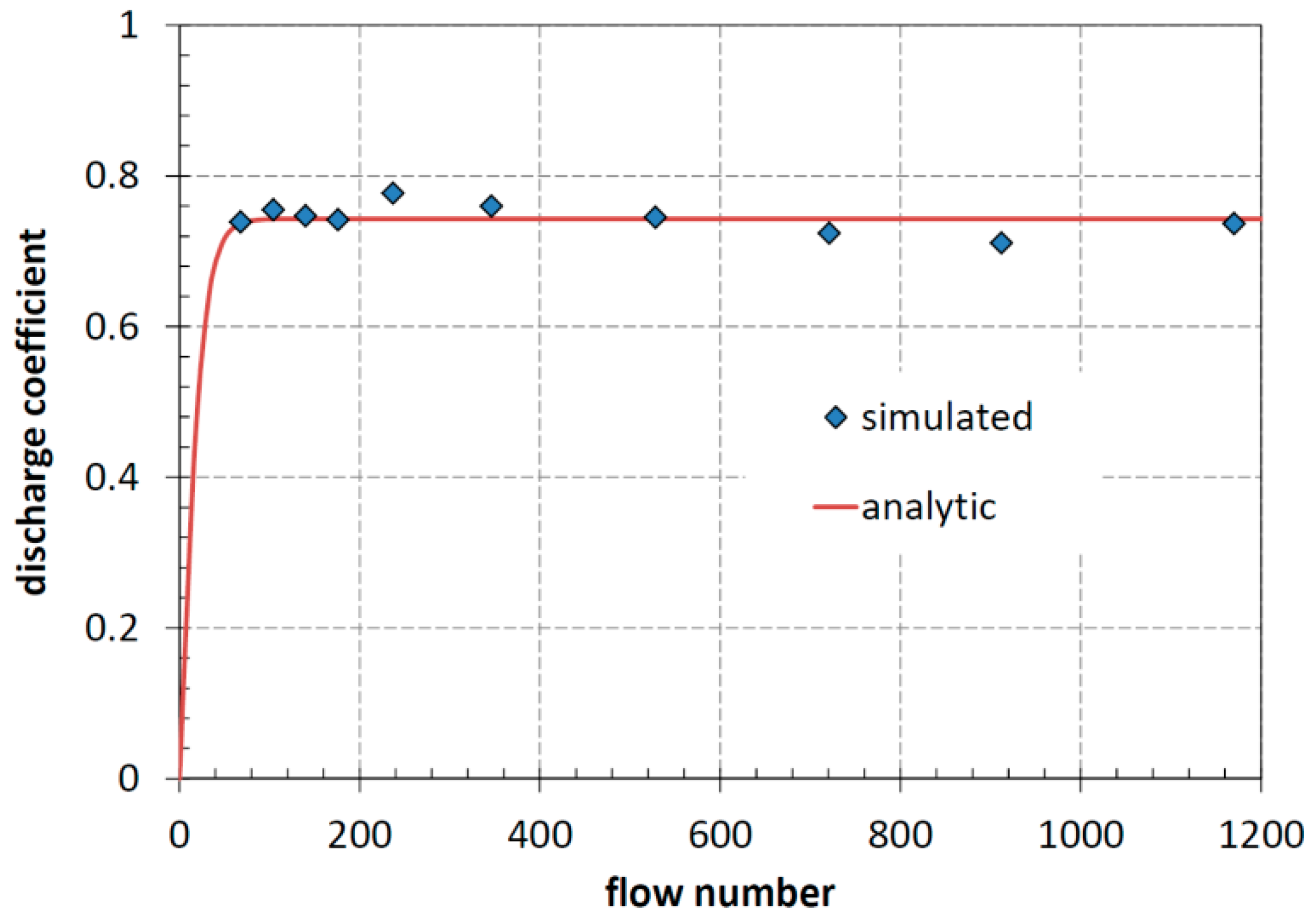
Hence, the discharge coefficient was calculated with the Equation (27):
where Qv is the flow rate through the valve imposed as boundary condition. The discharge coefficient is function of the flow number defined as:
being dh the hydraulic diameter and ν the kinematic viscosity. In LMS Amesim, the relationship between the discharge coefficient and the flow number is approximated by the Equation (29):
where λc is the critical flow number. In Figure 12 the values of the discharge coefficient simulated with the CFD code (dots) are reported. In the same graph the Equation (29) is plotted with Cd,max = 0.74 and λc = 50 in order to fit the calculated points. From the graph it is possible to notice that any value of λc lower than 50 could be acceptable, however it is worthless to investigate more in detail in that range, since the flow rate is extremely low.
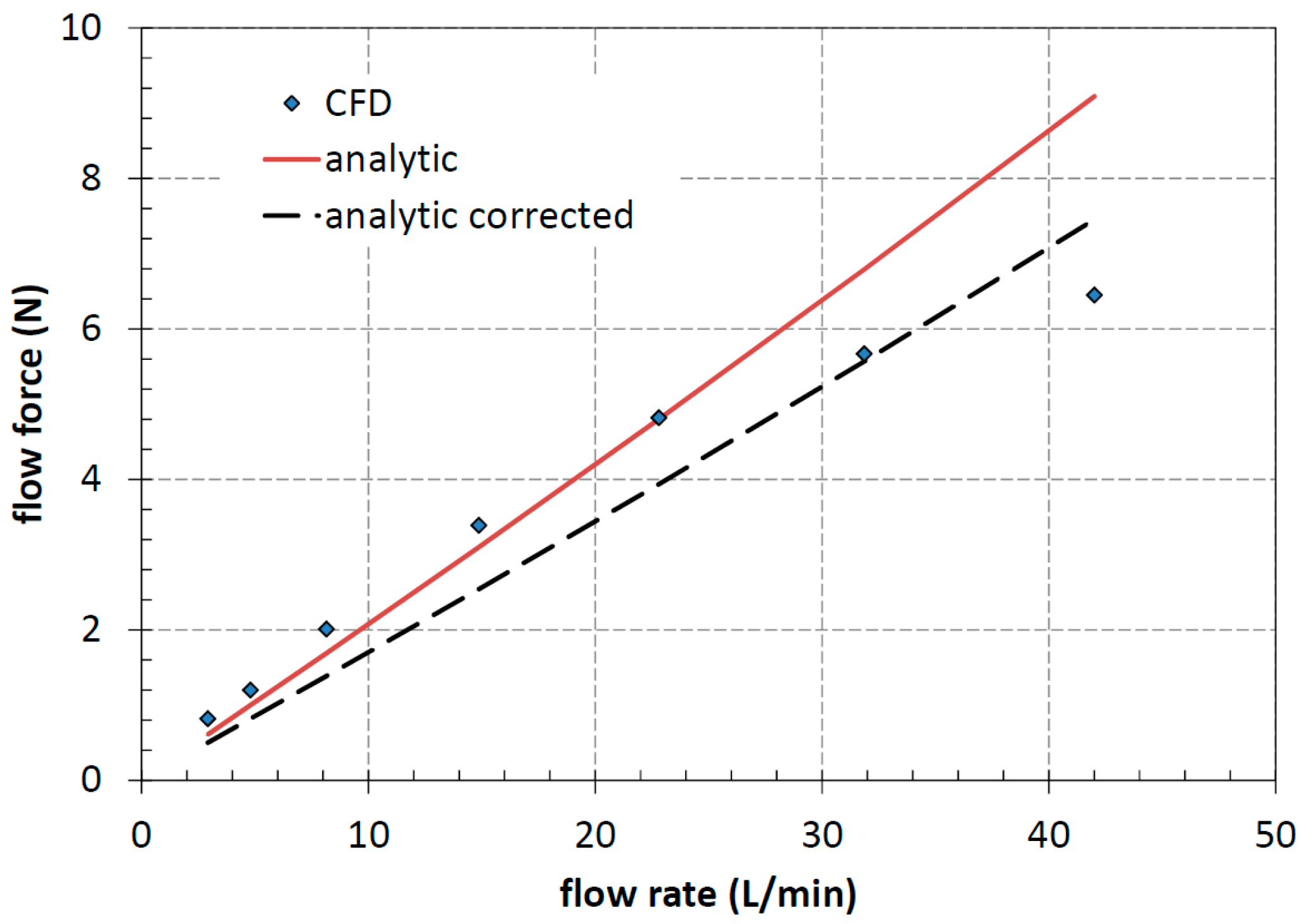
The flow force on the valve was evaluated as the difference between the theoretical opening force calculated assuming that a uniform pressure distribution exists on the spool surface, and the force FCFD calculated by the CFD code:
where ds is the spool diameter. The flow force is caused by the change of fluid momentum and the analytic expression is given by the Equation (31):
where υ is the flow velocity in the vena contracta, namely at the valve outlet, and ϑ the jet angle with respect to the spool axis. In Figure 13 the flow force calculated with the Equation (31), red curve, is contrasted with the values obtained by the Equation (30). It can be observed that up to 23 L/min the agreement is very good, while for higher flow rates the values calculated with the CFD code are lower. This predictable discrepancy is explained by the fact that the Equation (31) implemented in the Amesim model does not take into account the axial component of the fluid velocity at the valve inlet, since it assumes a radial entrance. On the contrary, in case of axial inlet as in the valve under study, an additional force partially compensates the closing force and this effect is higher as the flow rate increases [25].
To reproduce this behaviour it could be possible to improve the analytic model or to supply the flow force as a look-up table, but since in this case the difference is just a few Newton, it was decided to use the Equation (31) with a correction factor 0.82. In this way, it was possible to use the standard model available in the HCD Library.
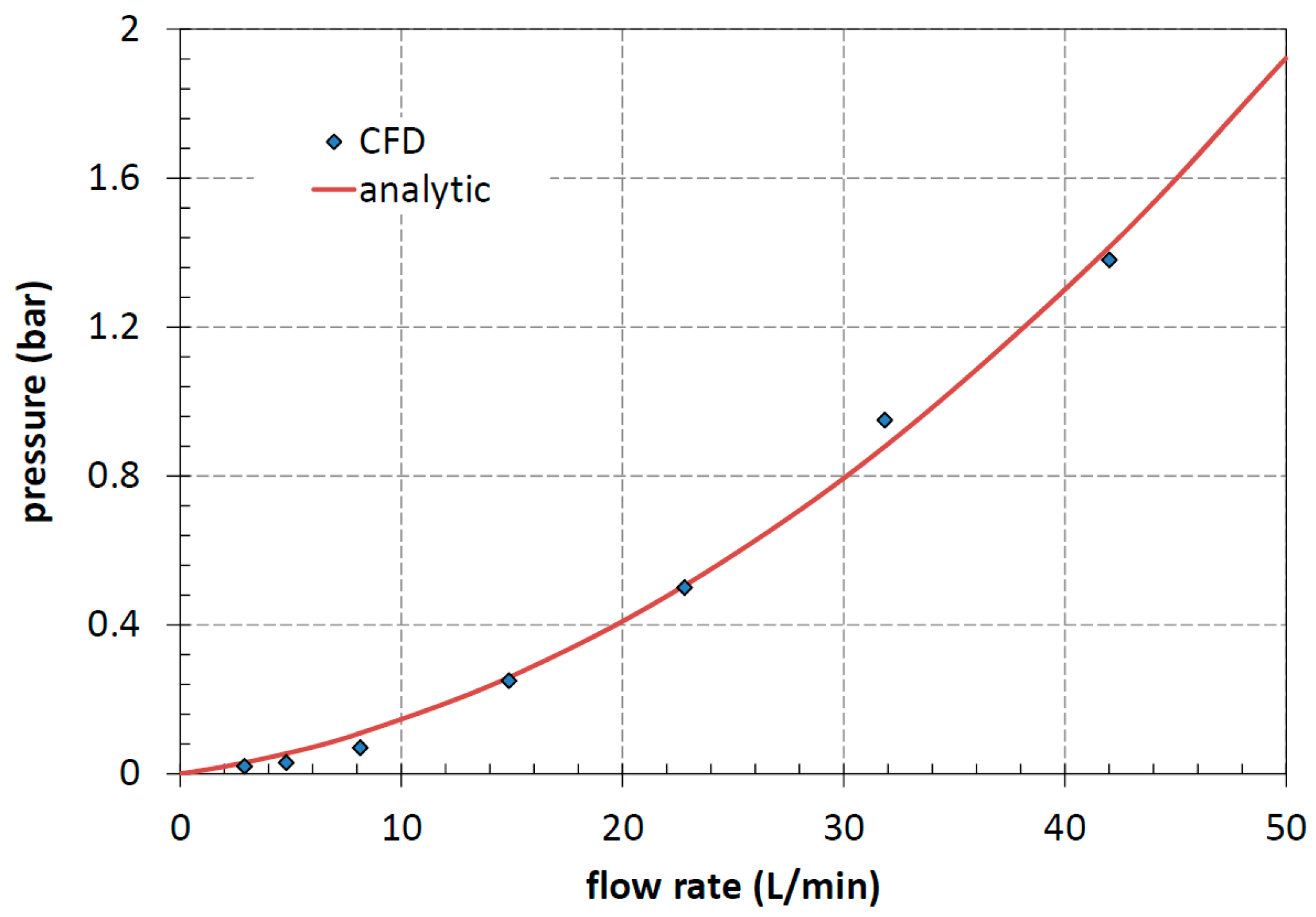
Finally, the most important aspect involves the evaluation of the pressure in the spring chamber, which can reach significant values compared to the pressure setting of the valve (6.5 bar). In Figure 14, the points simulated with FlowSimulation are plotted as function of the flow rate. In the lumped parameters model a 2nd order polynomial curve was used to interpolate the points.
5. Test Rig
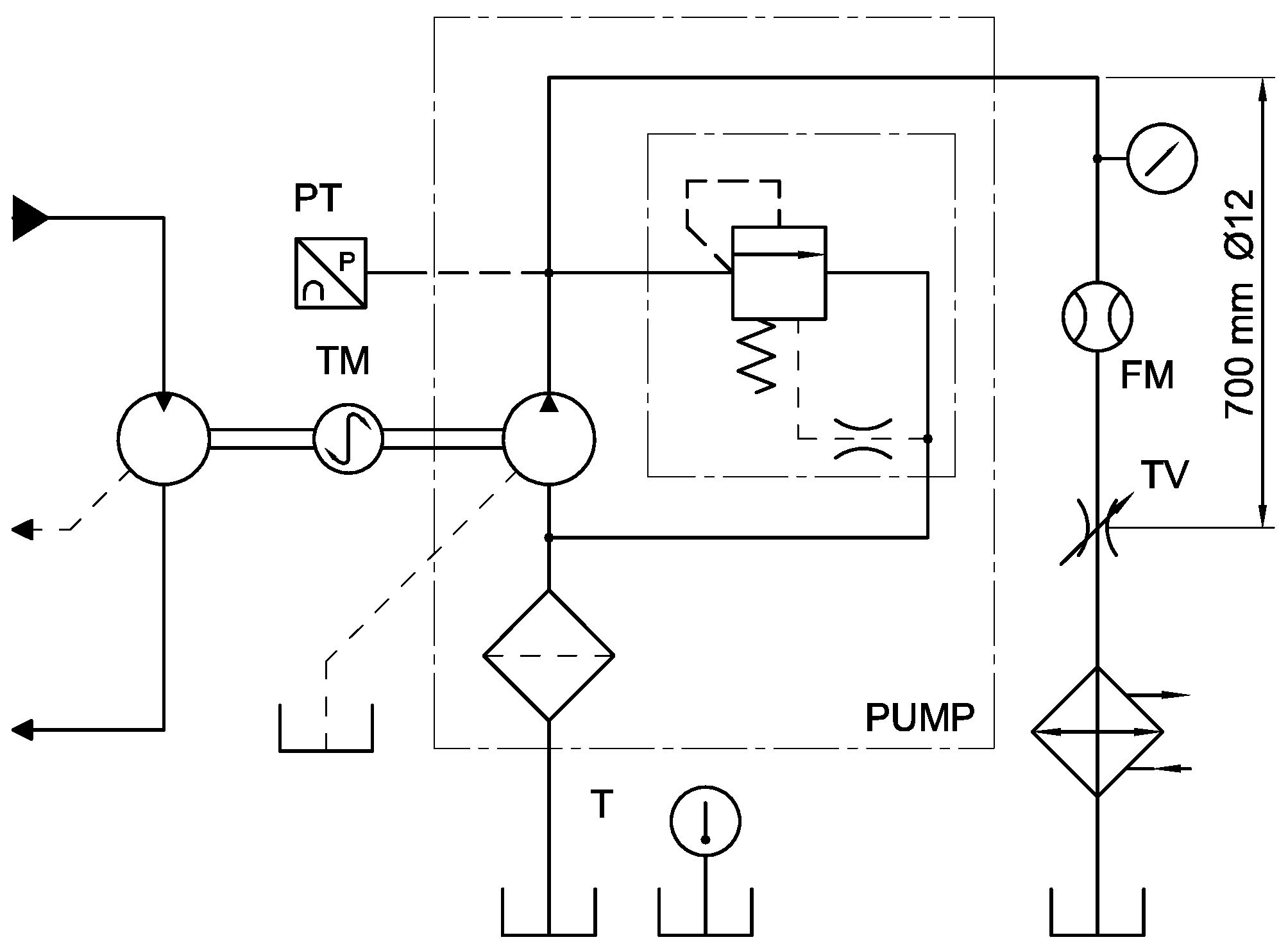
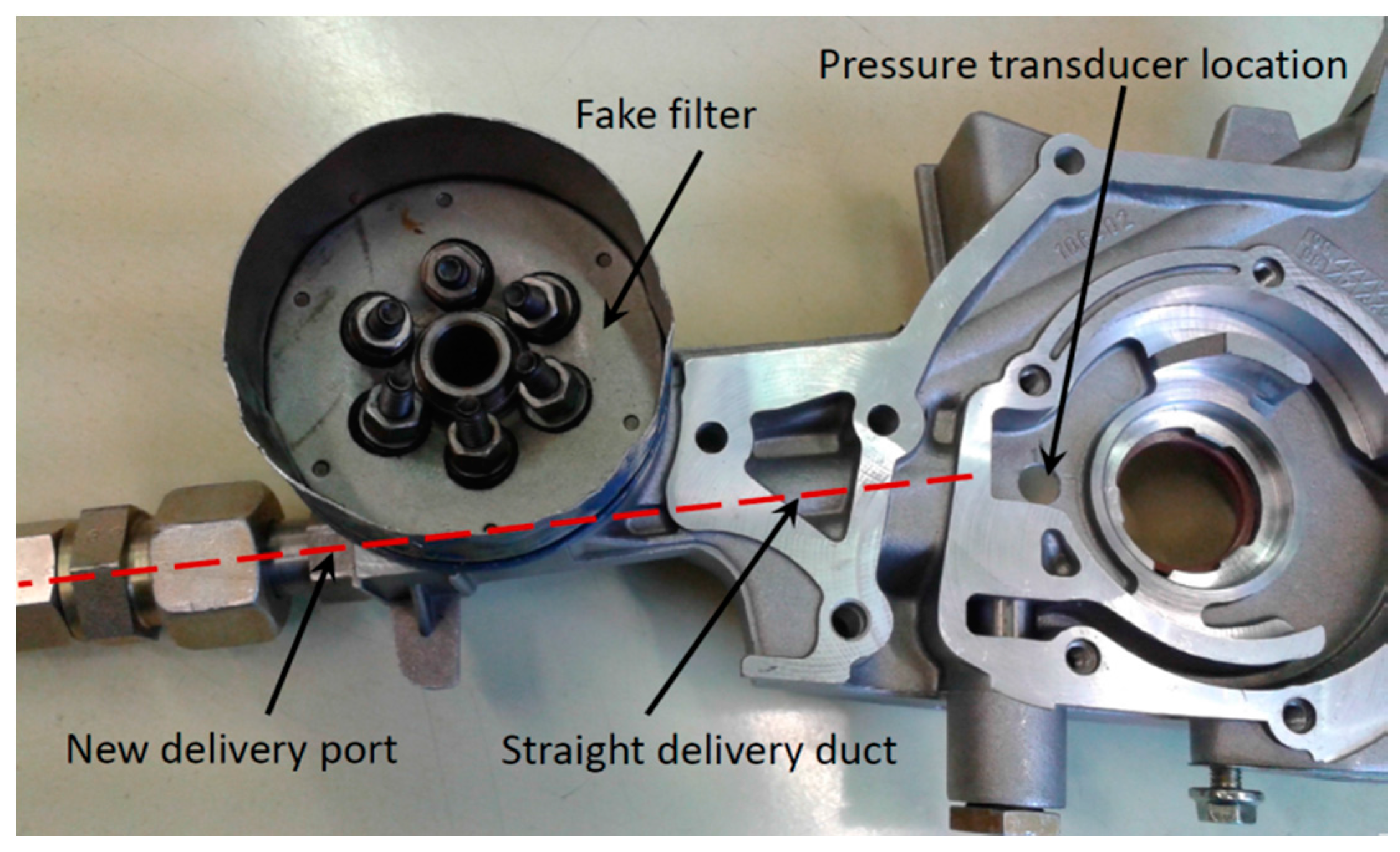
The pump was tested in order to determine the steady-state flow-pressure characteristic and the pressure ripple. The layout of the test rig is reported in Figure 15. The pump under test was driven by a fixed displacement bent-axis motor, which was fed by a variable flow hydraulic power unit. The speed and the torque on the driveline were measured by a torque meter VIBROMETER TG1 BP. The delivery pressure was measured by a strain-gauge transducer ENTRAN EPI M4 15 with measuring range 0–15 bar, mounted directly on the pump casing in the point indicated in Figure 16.
The flow rate was measured by a turbine flowmeter KEM KÜPPERS HM11 with measuring range 6–60 L/min. The load was simulated by a manual throttle valve. A water-oil heat exchanger was mounted on the return line and the temperature in the 5 L reservoir was measured by a PT100 resistance temperature detector. The tests were performed at the temperature of 65 °C and the oil was heated simply by dissipation in the throttle valve.
The working fluid was a 15W40 SAE grade lubricating oil with a viscosity of 35 cSt at 65 °C (measured with an Engler viscometer) and a density of 860 kg/m3. As shown in Figure 16, to simplify the delivery line, the filter was removed and substituted by a cover obtained by the casing of a filter with the inlet holes closed by bolts and O-rings. A new outlet line was created by removing the plug, indicated in Figure 1, at the end of the straight internal channel.
6. Complete Model and Validation
6.1. Model Description
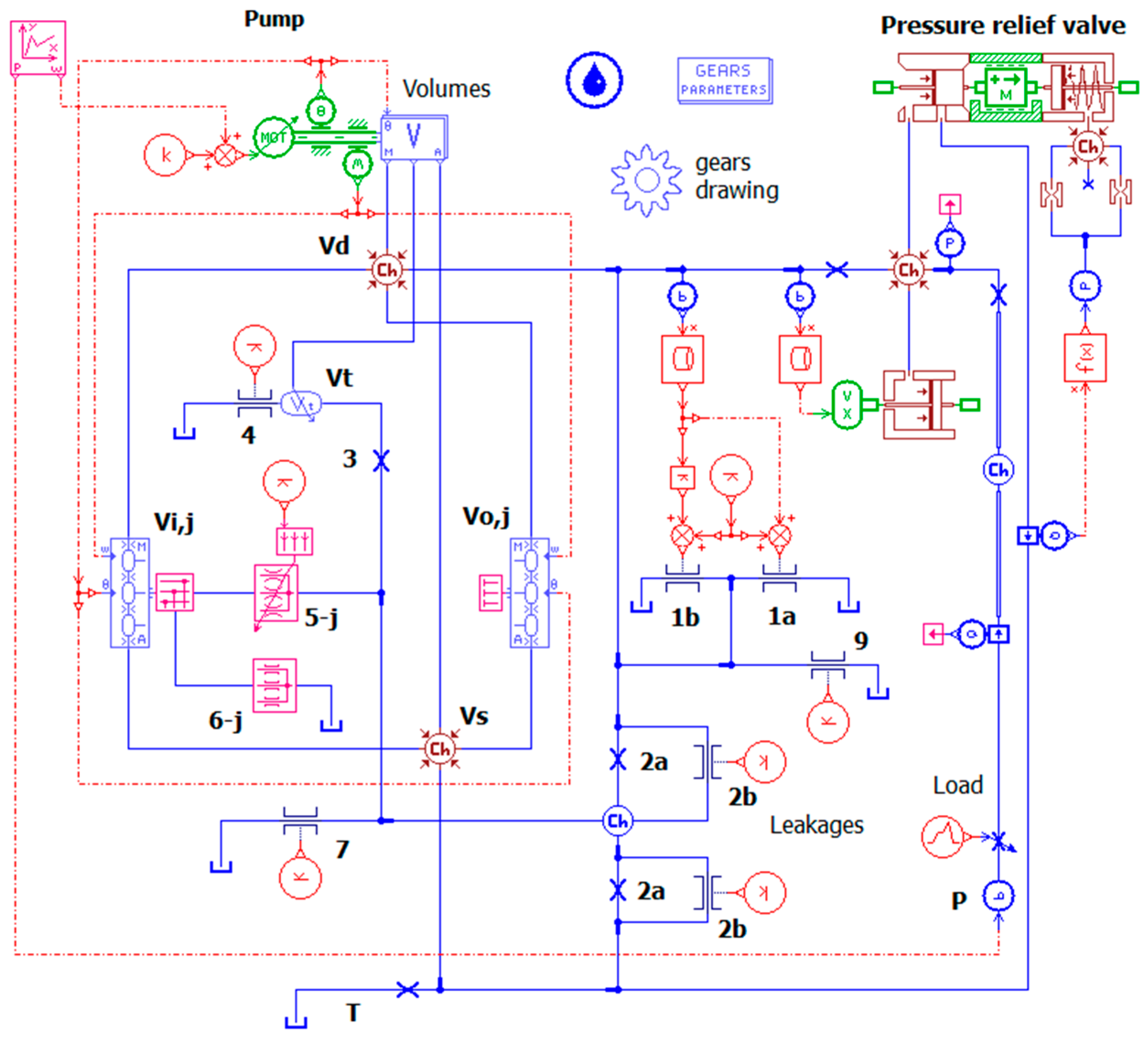
The model of the pump with the relief valve has been implemented in the LMS Amesim environment, making use of components belonging to the standard libraries as well as of new submodels in C code created with the Ameset tool. In Figure 17 a view of the entire model is shown. The delivery (Vd) and suction (Vs) volumes are simulated by a standard variable hydraulic capacity. They receive the volume derivative by a geometric component in which the Equations (3)–(5) are implemented. In turn, such component takes the main geometric parameters supplied by a specific icon.
The trapped volume is simulated by a customized component, which is able to manage the discontinuity in the differential equations when the volume is not defined. The main geometric parameters of the gears are listed in Table 3.
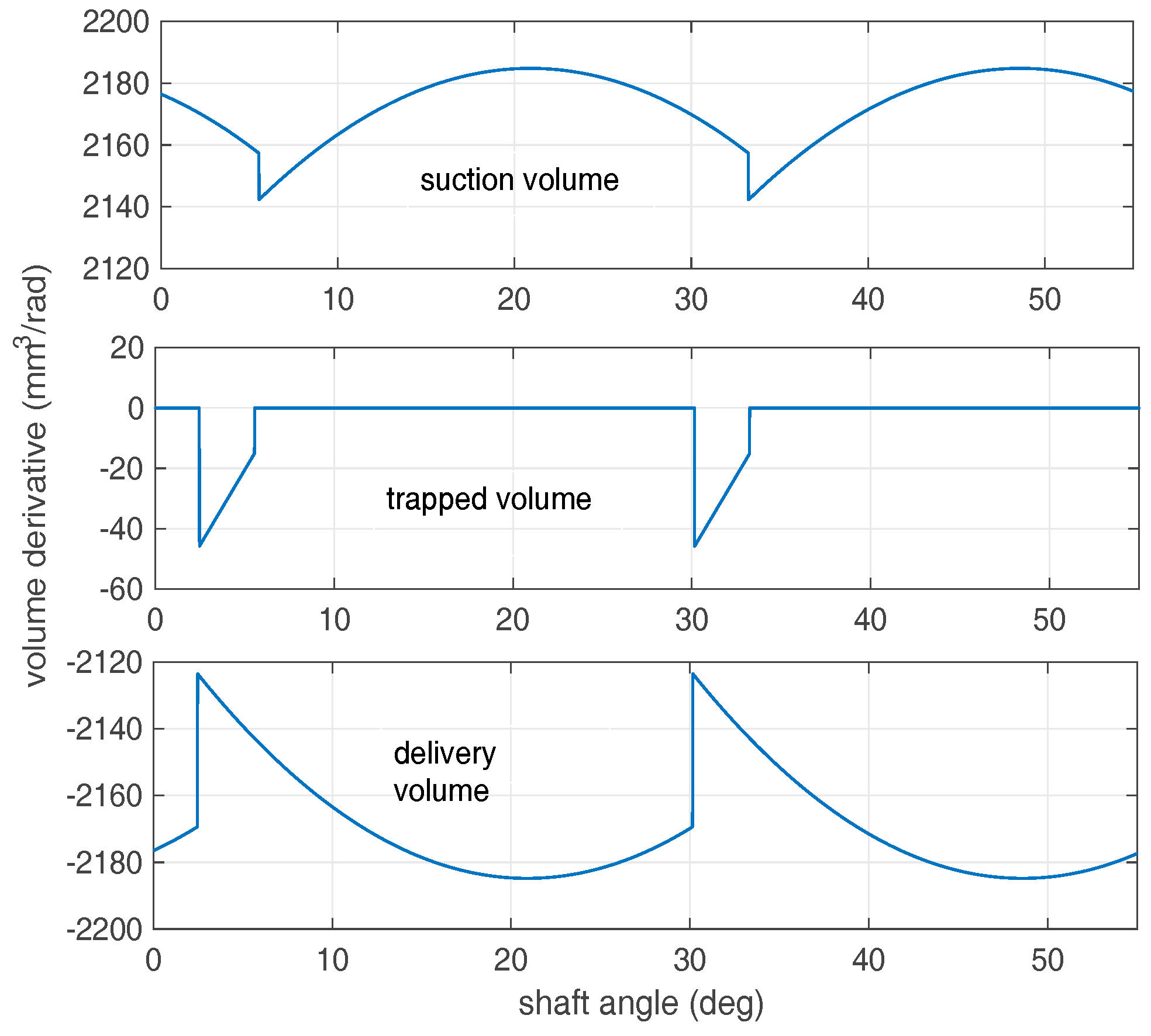
The volume derivatives for the pump under study as function of the shaft angle are reported in Figure 18. Since in this case the number of teeth of the inner gear is 13, the geometric functions are periodic of . By definition, the delivery volume derivative is always negative, while the suction is always positive. The discontinuities in the functions are related to the existence of the trapped volume. In particular, the discontinuity on the delivery volume is because a new contact point is generated and a fraction of the volume is now accounted in the trapped volume, which starts to exist. On the contrary, the discontinuity in the suction function indicates the detachment of a couple of teeth, hence the trapped capacity ends existing and its volume is aggregated to the inlet volume. For the volumes V to be used in the denominator of the Equation (2), the corresponding derivatives have been integrated analytically and the proper constants relative to the aggregation or separation of the carry-over volumes have been added or subtracted. However, it was found that the use of the mean volume instead of its instantaneous value leads to the same result.
A customized component is used for the simulation of all carry-over volumes of each gear. It also includes the leakages on the tooth tips. In these components, the number of volumes, function on the number of teeth and of the port plate geometry, is a parameter. Such approach allows simulating pumps with different numbers of chambers without modifying the circuit. In fact, also the components simulating the laminar orifices for the leakages 5 and 6 in Figure 4 use the number of teeth as parameter.
All other leakages are simulated with laminar or turbulent orifices. The cover deformation as function of the delivery pressure is supplied as a data file and is used to correct the height of the gaps 1 based on the Equations (17) and (18) and also to generate an additional variation of the delivery volume. The pressure relief valve is simulated with the HCD library and the spring chamber pressure is supplied as a function (see also Figure 14) of the flow rate. The filter seat is simulated by a 70 cc fixed volume, while the upstream internal delivery duct is simulated by an IRC (resistive, capacitive and inertia effects) model with diameter 11 mm and length 130 mm. The straight pipe of the test rig is simulated by a CFD 1D Lax Wendroff model with 9 internal nodes; this number was automatically calculated by the code based on the geometry of the pipe, in order to have a ratio between the length and the diameter of the cells equal to 6.
6.2. Steady State Validation
The validation of the model consisted in the comparison of the flow rate supplied by the pump as function of the pressure imposed by the throttle valve at constant oil temperature. The test was performed at 4 different pump speeds by progressively reducing the flow area of the throttle valve from the maximum opening up to the complete closing. For each position of the valve, the mean values of the flow rate and the pressure sensed by the transducer in the delivery volume were recorded. The obtained flow-pressure curves allow the validation of the total leakage flows and of the pressure value regulated by the relief valve.
However, for the first aspect, a tuning of the relative position of the gears within the geometric tolerances was necessary. In fact, even if generally the real clearances between the gears and the casing are known, how the total axial clearance is split between the two sides of the gears cannot be determined a priori. A similar uncertainty occurs for the position of the gears axes due to the radial clearances. Moreover, being in this case the gears not axially balanced, since the cover plate is flat, the usual assumption that the clearance is the same on the two sides could be not realistic. It is more likely that, since on the casing side the teeth of the inner gear are exposed entirely to the delivery pressure, the gear could be pushed against the cover. Based on this assumption, the value of the clearance ha2 used in the Equations from (19) to (21) was set equal to the total axial clearance (considering also the thermal expansion), while for the Equations (17) and (18) only the additional clearance due to the cover deformation was used for the gap. As far as the tip clearances hti and hto between the teeth and the crescent, their values has been set to about 75% of the maximum clearance in order to best fit the experimental data.
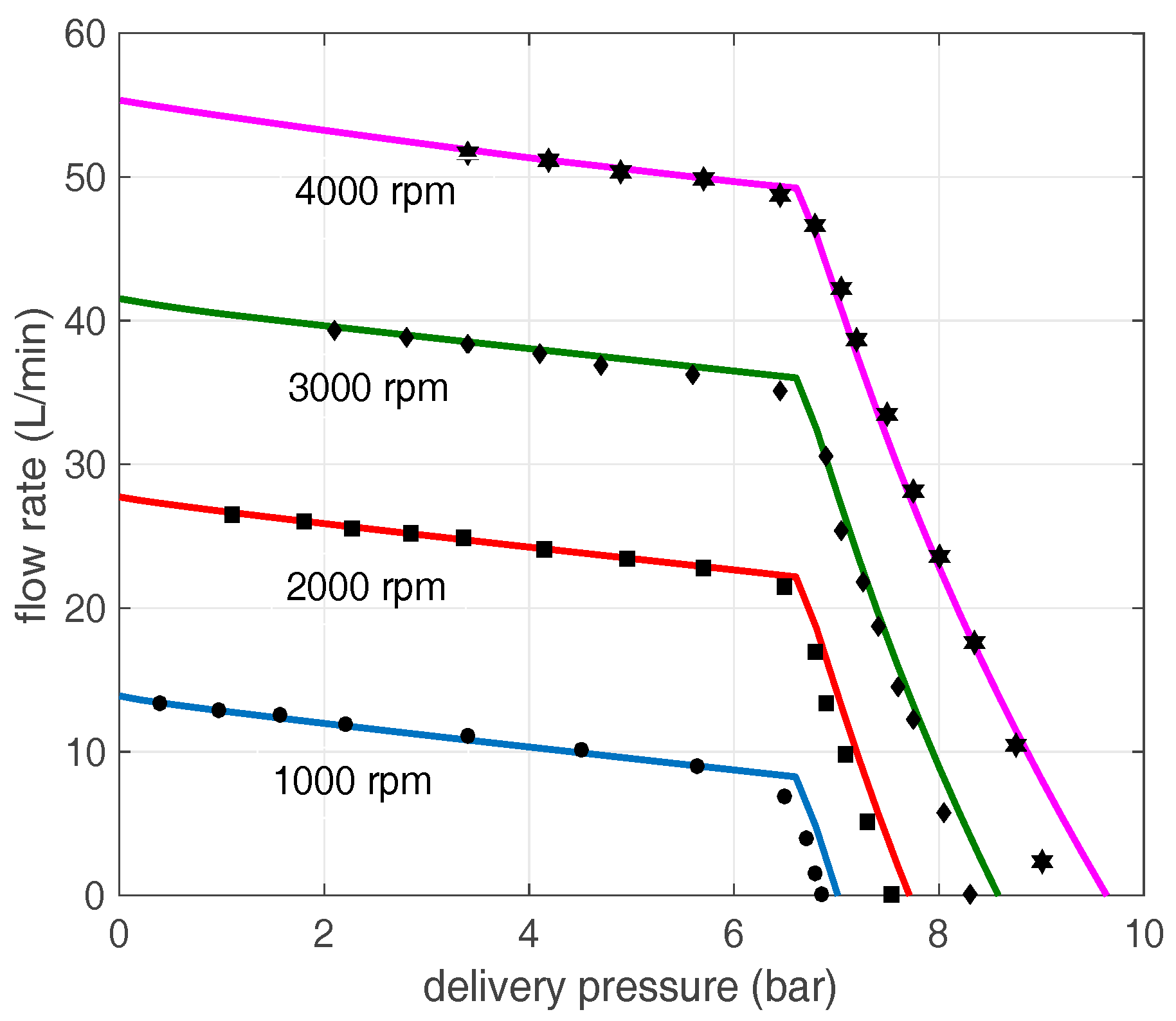
The comparison between the experimental (dots) and simulated (continuous lines) flow-pressure characteristics are shown in Figure 19.
It was not possible to impose inside the pump a low pressure at high speed due to the pressure drops in the delivery pipe. Below about 6.5 bar the pressure relief valve remains closed, hence the reduction of the flow rate is only due to the leakages.
When the pressure relief valve regulates, the pressure continues to increase, up to 9 bar at 4000 rpm, due to the increment of the spring force, of the flow forces and of the pressure in the spring chamber. A significant error in the evaluation of the regulated pressure is evident in the last part of the curves, in particular at 4000 rpm. However, it must be considered that in this condition most of the flow rate generated by the pump was recirculated internally, without flowing through the heat exchanger. In this way it was not possible to get under control the oil temperature, therefore it is likely that the last experimental points are not reliable, being obtained with a higher temperature.
The model allowed estimating that roughly 1/3 of the leakages are due to the axial clearances and 2/3 to the radial gaps. It is evident that the axial leakages give a significant contribution that cannot be neglected. Overall, the most important contribution to the leakages is due to the clearance between the tooth tips and the crescent, being about 50% of the total. This loss can be reduced, at equal values of clearances, by increasing the length of the crescent, in order to increment the number of teeth in contact with it, namely the number of carry-over volumes. In Table 4, the results of a sensitivity analysis on the percent reduction of the tooth tip leakage are shown. The angular extension of the crescent was used as variable parameter, with a consequence on the mean number of contact points over an angular pitch.
6.3. Dynamic Validation
The model is able to reproduce the instantaneous flow rate, which interacts with the resistance induced by the circuit and generates a pressure ripple. It is well known that the dynamic behaviour of a hydraulic line is highly influenced by the fluid bulk modulus, which in turn is very sensitive to the amount of undissolved air. It is likewise acknowledged that the determination of the amount of air and of the values of the time constants for the separation and dissolution of the air in the oil is still an open issue. Therefore, in this study the oil bulk modulus was determined in order to have the best agreement with the experimental pressure oscillations. The model of fluid implemented in LMS Amesim calculates the bulk modulus of the mixture air-oil as function of the current pressure and the equilibrium conditions given by the Henry’s law; moreover, the dissolution and separation of the air is considered instantaneous.
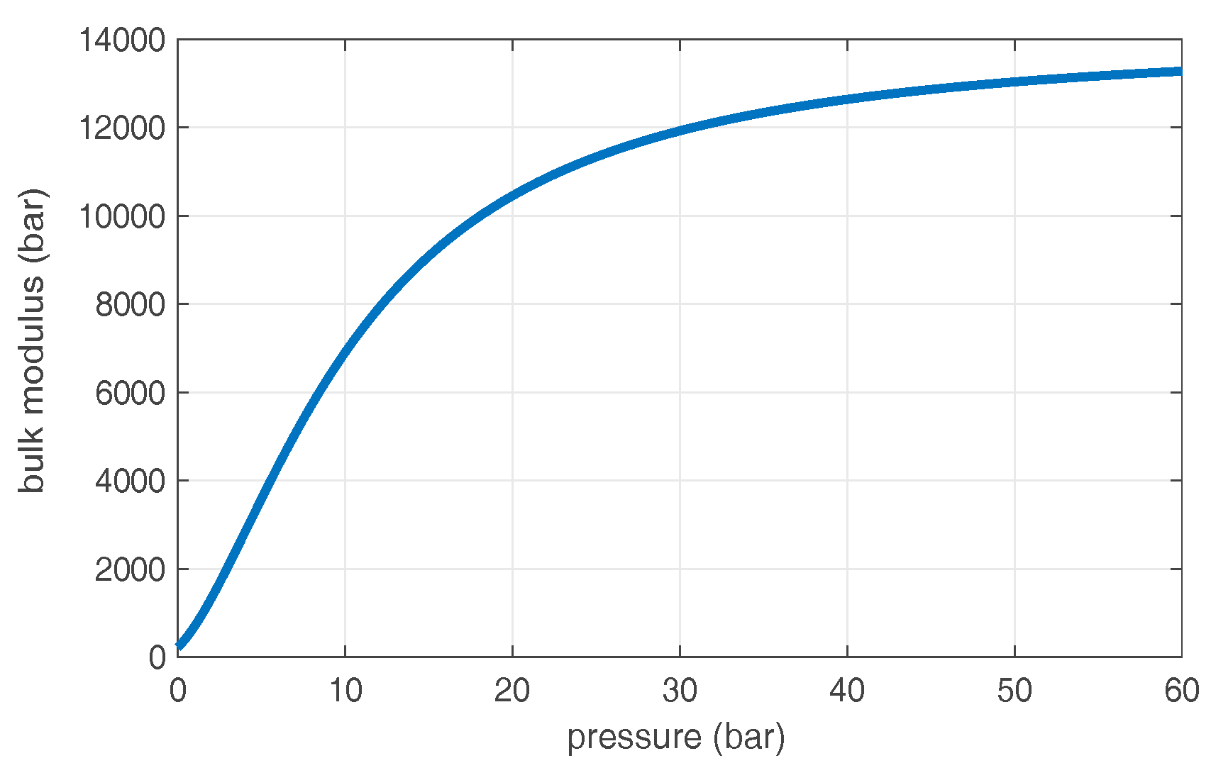
Since it is not realistic to consider only pure oil in the circuit, in order to take into account the presence of air bubbles in the delivery line, the fluid parameters were set in order to obtain the relationship between the bulk modulus and the pressure shown in Figure 20.
In particular, depending on the dynamics of the system under study, it is advised [26] to set the pressure at which all gas is dissolved (saturation pressure) to a very high value, up to 5000 bar for very fast acting systems and an amount of air in volume ranging from 0.1% to 1%. In this case, a saturation pressure of 1000 bar and an air percentage of 0.5% were used.
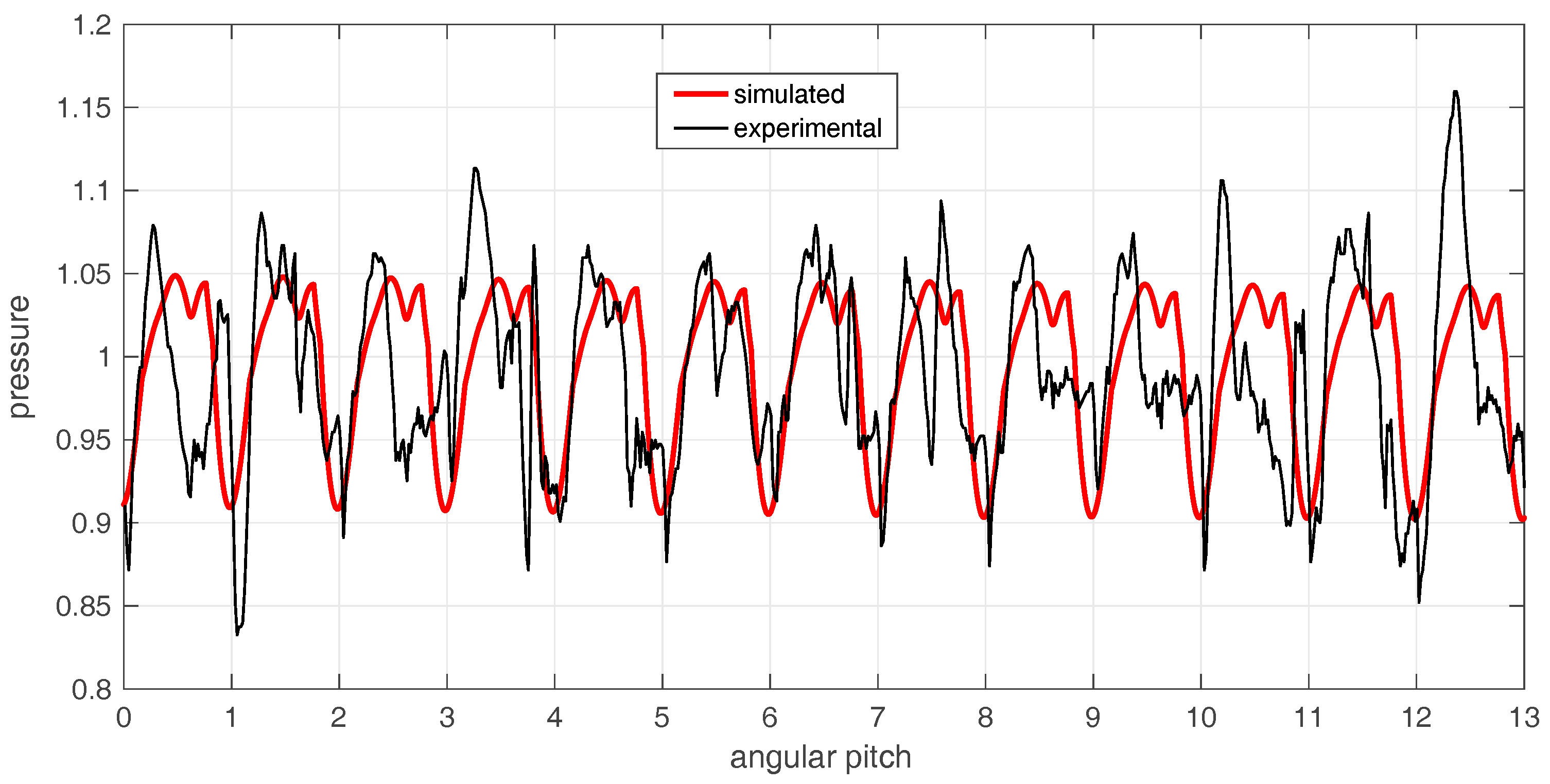
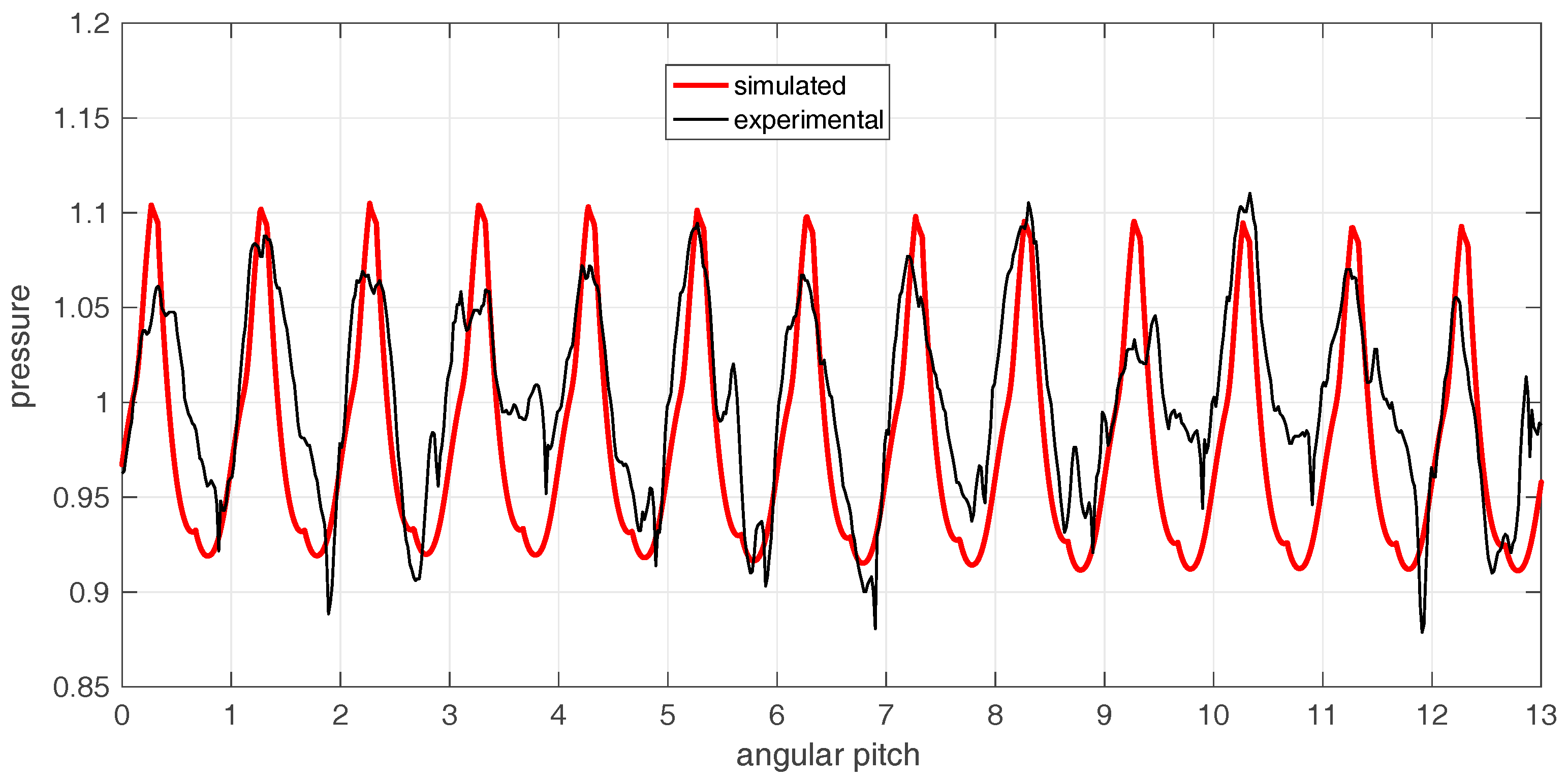
In this way for the pressure range of the pump under test, the bulk modulus varies between 3000 and 6000 bar, against the value of 14,000 bar of the pure oil. In Figure 21 the comparison between the simulated and the measured pressure ripple is shown for an entire shaft revolution, corresponding to 13 angular pitches of the driving gear, at 2000 rpm and with a mean delivery pressure of 3 bar. In Figure 22 the same comparison is shown at 4000 rpm and 6 bar. The graphs are normalized with respect to the mean value.
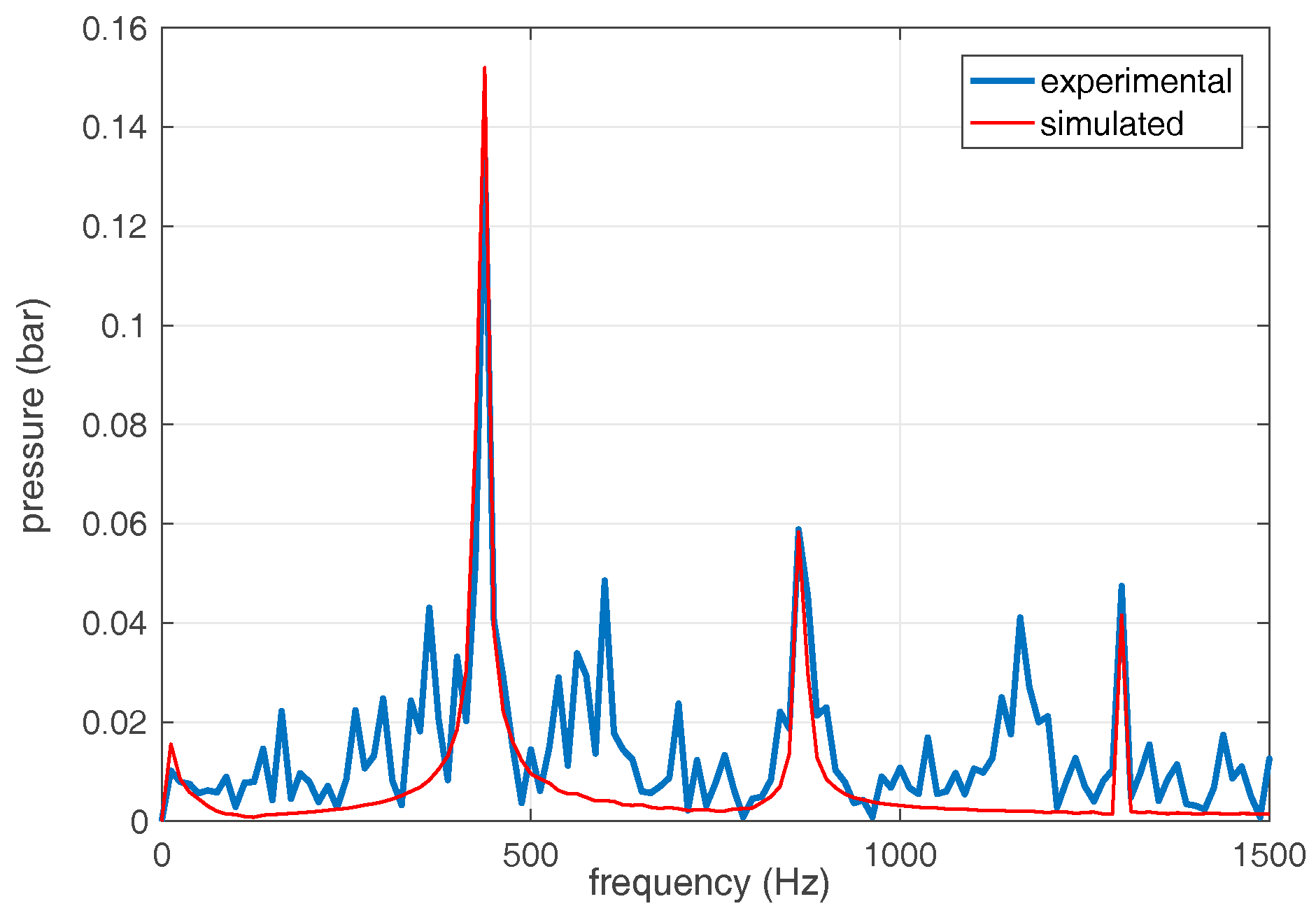
At low speed, the amplitude of the pressure oscillations is quite small and the shape of each wave is rather random, therefore this measurement could not be suitable to validate the model. However if the frequency domain is considered (Figure 23), it can be noticed that the three main frequencies are reproduced correctly by the model.
The dominant frequency is calculated with the Equation (32):
which at 2000 rpm gives 433.3 Hz. The other two frequencies are the 2nd and the 3rd harmonic, respectively 866.7 Hz and 1300 Hz. Some other frequencies, present in the experimental data, are not reproduced by the model. It is straightforward that the shape of the oscillations is highly influenced by the value of the bulk modulus.
7. Conclusions
The lumped parameters model of a crescent pump developed in the LMS Amesim environment has been presented. The approach used for the construction of the model consists in the identification of only three variable control volumes regardless of the number of teeth of the gears. The volume derivatives are calculated as function of the equation of the line of contact. The volumes isolated by the crescent are simulated by a customized component able to manage multiple hydraulic capacities is series.
It is possible to simulate pumps with different number of chambers without modifying the layout of the model, since the number of teeth is supplied as a parameter.
Particular attention has been paid for the simulation of the leakages, because the pump used as reference is not gap-compensated. For the axial gaps between the gears and the housing two critical issues emerged. The first aspect is the deformation of the cover plate, which generates an increment of the gap height of the same order of magnitude of the manufacturing tolerances. To solve this first problem the gap height has been considered variable with the delivery pressure based on the validated outcomes from a FEM analysis. The second issue is the uncertainty of the position of the gears with respect to the casing, since the rotors are not axially balanced. In this case, a reasonable assumption has been made. The same uncertainty is due to the radial position of the gears with a consequence on the operating tooth tip clearance. This value was tuned on the experimental data in order to fit the reduction of the delivered flow rate as function of the pressure. This aspect could be a topic of further studies, for instance using a multi domain approach, which could involve the dynamics of the gears under the action of the pressure forces and the tooth contact analysis.
As far as the integrated pressure relief valve is concerned, a critical aspect is the pressurization of the spring chamber. In fact, the additional closing force can alter significantly the steady-state characteristic of the valve for high values of discharged flow rates. Good results have been obtained with some CFD simulations with a fixed position of the spool.
The authors are aware of some intrinsic limitations of the approach used for modelling the pump. Because the control volumes are not connected one to each other through flow areas, but they evolve independently, it is not possible to simulate the incomplete filling of the pump at high rotational speed. Moreover, a possible pressure peak in the meshing zone cannot be reproduced. Nevertheless, the merit of the model is a very fast computational time and a good reliability in non-extreme operating conditions. It can be useful when it is necessary to simulate the pump as a source of flow ripple in a quite complex circuit.
Acknowledgments
This research did not receive any specific grant from funding agencies in the public, commercial, or not-for-profit sectors.
Author Contributions
Massimo Rundo developed the mathematical model of the pump and performed the experiments; Alessandro Corvaglia developed the FEM and CFD models; both implemented the model of the pump in Amesim; Massimo Rundo wrote the paper.
Conflicts of Interest
The authors declare no conflict of interest.
Abbreviations
The following abbreviations are used in this manuscript:
| Av | flow area of the relief valve |
| b1 | distance between two consecutive teeth of the inner gear |
| b2 | root thickness of the teeth of the inner gear |
| b3 | extension of the inner rim of the casing exposed to the delivery pressure |
| b4 | width of the equivalent rectangular gap for the leakage on the tooth face of the inner gear |
| Cd | discharge coefficient |
| Cd,max | maximum value of the discharge coefficient |
| ds | valve spool diameter |
| dh | hydraulic diameter of the valve flow area |
| e | eccentricity between the gears |
| f | dominant frequency of the pressure signal |
| FCFD | force on the frontal surface of the spool calculated by the CFD model |
| Fjet | flow force |
| l1 | length of the leakage passage between delivery volume and sump, cover side |
| l2 | length of the leakage passage between annular volume and sump |
| l3 | length of the leakage passage between delivery volume and annular volume |
| l4 | length of the leakage passage between delivery volume and sump, tooth face, cover side |
| l5 | length of the leakage passage between the outer gear and the casing |
| lti, lto | thickness of the tooth tip of the inner/outer gear respectively |
| ha1, ha2 | axial clearance on the cover/housing side respectively |
| hri | radial clearance of the driving collar of the inner gear |
| hre | radial clearance between the outer gear and the casing |
| hti, hto | clearance between the tooth tip and the crescent for the inner/outer gear respectively |
| H | gears thickness |
| nt | mean number of teeth of the inner gear exposed to the delivery pressure |
| Ni, No | maximum number of carry-over volumes belonging to the inner/outer gear respectively |
| p′ | pressure in the annular volume between the delivery volume and the sump |
| pd | delivery pressure |
| pt | trapped volume pressure |
| pT | sump pressure (atmospheric) |
| Qin, Qout | ingoing/outgoing flow rate in a control volume respectively |
| Qv | flow rate discharged by the relief valve |
| Rc | internal radius of the cover |
| Ri | radius of the driving collar of the inner gear |
| Rt1, Rt2 | tooth tip radius of the inner/outer gear respectively |
| Vd | delivery volume |
| Vi, Vo | carry-over volume belonging to the inner/outer gear respectively |
| Vs | suction volume |
| Vt | trapped volume |
| β | fluid bulk modulus |
| ε | eccentricity ratio of the outer gear with respect to the casing |
| δ1, δ2 | coordinate respectively of the first and second contact point along the line of contact |
| Δh | maximum deformation of the cover |
| Δφ | angular pitch of the inner gear |
| λ | flow number |
| λc | critical flow number |
| µ | fluid dynamic viscosity |
| φ | angular position of the shaft |
| θ | operating pressure angle |
| jet angle with respect to the spool axis | |
| Ψd, Ψs | angles identifying the extension of the crescent |
| ρ | fluid density |
| ρ1, ρ2 | radius of the pitch circle of the inner/outer gear respectively |
| ρi1, ρi2 | vector ray of the inner gear for the contact points 1 and 2 respectively |
| ρo1, ρo2 | vector ray of the outer gear for the contact points 1 and 2 respectively |
| ν | kinematic viscosity |
| νd, νs | normalized angular position relative to the delivery/suction volume respectively |
| ν01, ν02 | constants for νd and νs respectively |
| τ | transmission ratio |
| ω | angular speed of the shaft |
References
- Mancò, S.; Nervegna, N.; Rundo, M.; Armenio, G.; Pachetti, C.; Trichilo, R. Gerotor Lubricating Oil Pump for IC Engines. SAE Trans. J. Engines 1998, 107, 2267–2284. [Google Scholar]
- Schweiger, W.; Vacca, A. Gerotor Pumps for Automotive Drivetrain Applications: A Multi Domain Simulation Approach. SAE Int. J. Passeng. Cars 2011, 4, 1358–1376. [Google Scholar] [CrossRef]
- Garcia-Vilchez, M.; Gamez-Montero, P.; Codina, E.; Castilla, R.; Raush, G.; Freire, J.; Rio, C. Computational Fluid Dynamics and Particle Image Velocimetry Assisted Design Tools for a New Generation of Trochoidal Gear Pumps. Adv. Mech. Eng. 2015, 7, 1–14. [Google Scholar] [CrossRef] [Green Version]
- Altare, G.; Rundo, M. Computational Fluid Dynamics Analysis of Gerotor Lubricating Pumps at High Speed: Geometric Features Influencing the Filling Capability. J. Fluids Eng. 2016, 138, 111101. [Google Scholar] [CrossRef]
- Demenego, A.; Vecchiato, D.; Litvin, F.; Nervegna, N.; Mancò, S. Design and Simulation of Meshing of a Cycloidal Pump. Mech. Mach. Theory 2002, 37, 311–332. [Google Scholar] [CrossRef]
- Bonandrini, G.; Mimmi, G.; Rottenbacher, C. Theoretical Analysis of Internal Epitrochoidal and Hypotrochoidal Machines. J. Mech. Eng. Sci. 2009, 223, 1469–1480. [Google Scholar] [CrossRef]
- Gamez-Montero, P.; Castilla, R.; Khamashta, M.; Codina, E. Contact Problems of a Trochoidal-Gear Pump. Int. J. Mech. Sci. 2006, 48, 1471–1480. [Google Scholar] [CrossRef]
- Inaguma, Y. Friction Torque Characteristics of an Internal Gear Pump. J. Mech. Eng. Sci. 2011, 225, 1523–1534. [Google Scholar] [CrossRef]
- Rundo, M.; Nervegna, N. Lubrication Pumps for Internal Combustion Engines: A Review. Int. J. Fluid Power 2015, 16, 59–74. [Google Scholar] [CrossRef]
- Mimmi, G.; Pennacchi, P. Involute Gear Pumps versus Lobe Pumps: A Comparison. J. Mech. Des. 1997, 119, 458–465. [Google Scholar] [CrossRef]
- Zhou, H.; Song, W. Theoretical Flowrate Characteristics of the Conjugated Involute Internal Gear Pump. J. Mech. Eng. Sci. 2013, 227, 730–743. [Google Scholar] [CrossRef]
- Zhou, H.; Song, W. Optimization of Floating Plate of Water Hydraulic Internal Gear Pump. In Proceedings of the 8th JFPS International Symposium on Fluid Power, Okinawa, Japan, 25–28 October 2011.
- Song, W.; Zhou, H.; Zhao, Y. Design of the Conjugated Straight-Line Internal Gear Pairs for Fluid Power Gear Machines. J. Mech. Eng. Sci. 2013, 227, 1776–1790. [Google Scholar] [CrossRef]
- Slodczyk, D.; Stryczek, J. Fundamentals of Designing the Internal Involute Gearing Pumps. In Proceedings of the 7th FPNI Ph.D. Symposium on Fluid Power, Reggio Emilia, Italy, 27–30 June 2012.
- Fetvaci, C. Computerised Tooth Profile Generation of Conjugated Involute Internal Gears. Key Eng. Mater. 2014, 572, 355–358. [Google Scholar] [CrossRef]
- Jiang, Y.; Furmanczyk, M.; Lowry, S.; Zhang, D.; Perng, C. A Three-Dimensional Design Tool for Crescent Oil Pumps; SAE Technical paper 2008-01-0003; Society of Automotive Engineers: Warrendale, PA, USA, 2008. [Google Scholar]
- Guo, J.; Liu, L.; Chen, P.; Zhao, Q. Flow Field Numerical Simulation of Straight Line Conjugate Internal Meshing Gear Pump. Appl. Mech. Mater. 2013, 433–435, 40–43. [Google Scholar] [CrossRef]
- Mancò, S.; Nervegna, N. Simulation of an External Gear Pump and Experimental Verification. In Proceedings of the JFPS International Symposium on Fluid Power, Tokyo, Japan, 13–16 March 1989.
- Rundo, M. Theoretical Flow Rate in Crescent Pumps. Simul. Model. Pract. Theory 2016, in press. [Google Scholar]
- Rundo, M. Energy Consumption in ICE Lubricating Gear Pumps; SAE Technical Paper 2010-01-2146; Society of Automotive Engineers: Warrendale, PA, USA, 2010. [Google Scholar]
- Kini, S.; Mapara, N.; Thoms, R.; Chang, P. Numerical Simulation of Cover Plate Deflection in Gerotor Pump; SAE Technical Paper 2005-01-1917; Society of Automotive Engineers: Warrendale, PA, USA, 2005. [Google Scholar]
- Nanè, P. CFD Codes Comparison for Flow Simulation Problems on Fluid Power Components. Master’s Thesis, Politecnico di Torino, Turin, Italy, March 2016. [Google Scholar]
- Sobachkin, A.; Dumnov, G. Numerical Basis of CAD-Embedded CFD. In Proceedings of the NAFEMS World Congress, Salzburg, Austria, 9 June 2013.
- Altare, G.; Rundo, M. 3D Dynamic Simulation of a Flow Force Compensated Pressure Relief Valve. In Proceedings of the ASME 2016 International Mechanical Engineering Congress and Exposition, Phoenix, AZ, USA, 11–17 November 2016.
- Finesso, R.; Rundo, M. Numerical and Experimental Investigation on a Conical Poppet Relief Valve with Flow Force Compensation. Int. J. Fluid Power 2016, in press. [Google Scholar]
- Siemens Industry Software NV. LMS Imagine.Lab Amesim—Hydraulic Library User’s Guide; Siemens Industry Software NV: Leuven, Belgium, 2016. [Google Scholar]
Figure 1.
3D drawing of the crescent pump under study with the indication of flow path (red lines).

Figure 2.
Definition of the control volumes.

Figure 3.
Line of contact, vector rays and auxiliary variables δ.

Figure 4.
Hydraulic scheme of the pump with the indication of all possible flow paths.

Figure 5.
Definition of the geometric parameters for the modelling of the leakages.

Figure 6.
Deformation field of the cover at 3 bar with the indication of the transducer location.

Figure 7.
Mounting of the proximity transducer on the test rig and position with respect to the pump. Figure unit = mm.
Figure 7.
Mounting of the proximity transducer on the test rig and position with respect to the pump. Figure unit = mm.

Figure 8.
Cross section of the relief valve with a detail of the bottom view.

Figure 9.
Pressure field with cell refinement across a hole with 2 L/min and lift of 0.35 mm.

Figure 10.
Regulated pressure at 2 L/min and lift 0.35 mm vs. number of cell in the minimum area.

Figure 11.
Velocity field at 1.25 mm and 30 L/min.

Figure 12.
Discharge coefficient vs. flow number: tuning of analytic model on CFD results.

Figure 13.
Flow force vs. flow rate: tuning of the analytic expression on CFD simulations.

Figure 14.
Spring chamber pressure vs. flow rate: fitting of CFD values with 2nd order polynomial.

Figure 15.
Hydraulic scheme of the test rig.

Figure 16.
Photo of the pump with the connection of the delivery line.

Figure 17.
Complete pump model in LMS Amesim.

Figure 18.
Derivatives of delivery, suction and trapped volumes vs. shaft angle.

Figure 19.
Simulated and measured steady state characteristics at 65 °C and four speed values.

Figure 20.
Bulk modulus as function of the pressure.

Figure 21.
Simulated and experimental instantaneous delivery pressure at 2000 rpm, 3 bar and 65 °C.

Figure 22.
Simulated and experimental instantaneous pressure at 4000 rpm, 6 bar and 65 °C.

Figure 23.
FFT of the pressure signal at 2000 rpm.


| Pressure (bar) | Measured (mm) | Simulated (mm) | Simulated Max (mm) |
|---|---|---|---|
| From 3 to 6 | 0.010 | 0.009 | 0.016 |
| From 3 to 8 | 0.017 | 0.018 | 0.028 |
| Configuration | Refinement B | Refinement C | No. Cells in the Minimum Area | No. Fluid Cells (1000×) |
|---|---|---|---|---|
| 1 | 0 | 0 | 2 | 1307 |
| 2 | 1 | 0 | 5 | 1326 |
| 3 | 1 | 1 | 7 | 1377 |
| 4 (Figure 9) | 2 | 1 | 13 | 1750 |
| 5 | 2 | 2 | 26 | 3102 |
| Parameter | Value |
|---|---|
| Number of teeth | 13/16 |
| Teeth normal module m0 (mm) | 4 |
| Normal pressure angle θ0 (deg) | 32 |
| Eccentricity e (mm) | 6 |
| Tooth tip radius of the driving gear Rt1 (mm) | 29.1 |
| Tooth tip radius of the driven gear Rt2 (mm) | 28.6 |
| Root radius of the driving gear Rf1 (mm) | 21.95 |
| Root radius of the driven gear Rf2 (mm) | 35.6 |
| Gears axial thickness H (mm) | 13 |
| Pump displacement (cc/rev) | 13.65 |
| Crescent Extension | No. Contact Points Driver Gear | No. Contact Points Driven Gear | Leakage Reduction (%) |
|---|---|---|---|
| 34° (current) | 1.22 | 1.85 | 0 |
| 40° | 1.44 | 2.18 | 20% |
| 46° | 1.65 | 2.51 | 34% |
| 52° | 1.87 | 2.84 | 50% |
© 2016 by the authors; licensee MDPI, Basel, Switzerland. This article is an open access article distributed under the terms and conditions of the Creative Commons Attribution (CC-BY) license (http://creativecommons.org/licenses/by/4.0/).
Share and Cite
MDPI and ACS Style
Rundo, M.; Corvaglia, A. Lumped Parameters Model of a Crescent Pump. Energies 2016, 9, 876. https://doi.org/10.3390/en9110876
AMA Style
Rundo M, Corvaglia A. Lumped Parameters Model of a Crescent Pump. Energies. 2016; 9(11):876. https://doi.org/10.3390/en9110876
Chicago/Turabian StyleRundo, Massimo, and Alessandro Corvaglia. 2016. "Lumped Parameters Model of a Crescent Pump" Energies 9, no. 11: 876. https://doi.org/10.3390/en9110876
Note that from the first issue of 2016, this journal uses article numbers instead of page numbers. See further details here.