Forecasting Crude Oil Price Using EEMD and RVM with Adaptive PSO-Based Kernels

Abstract

Crude oil, as one of the most important energy sources in the world, plays a crucial role in global economic events. An accurate prediction for crude oil price is an interesting and challenging task for enterprises, governments, investors, and researchers. To cope with this issue, in this paper, we proposed a method integrating ensemble empirical mode decomposition (EEMD), adaptive particle swarm optimization (APSO), and relevance vector machine (RVM)—namely, EEMD-APSO-RVM—to predict crude oil price based on the “decomposition and ensemble” framework. Specifically, the raw time series of crude oil price were firstly decomposed into several intrinsic mode functions (IMFs) and one residue by EEMD. Then, RVM with combined kernels was applied to predict target value for the residue and each IMF individually. To improve the prediction performance of each component, an extended particle swarm optimization (PSO) was utilized to simultaneously optimize the weights and parameters of single kernels for the combined kernel of RVM. Finally, simple addition was used to aggregate all the predicted results of components into an ensemble result as the final result. Extensive experiments were conducted on the crude oil spot price of the West Texas Intermediate (WTI) to illustrate and evaluate the proposed method. The experimental results are superior to those by several state-of-the-art benchmark methods in terms of root mean squared error (RMSE), mean absolute percent error (MAPE), and directional statistic (Dstat), showing that the proposed EEMD-APSO-RVM is promising for forecasting crude oil price.

1. Introduction

It was reported by British Petroleum (BP) that fossil fuels accounted for 86% of primary energy demand in 2014 and remain the dominant source of energy powering the global economy, with almost 80% of total energy supply in 2035. Among fossil fuels, crude oil is and will be the most important energy source, accounting for almost 29% of total energy supply in 2035 [1], and plays a vital role in all economies. In light of the importance of crude oil for the global economy, many enterprises, governments, investors, and researchers have devoted great efforts to building models to predict its price and volatility. However, due to its complexity, the price of oil can be easily affected by many factors, such as supply and demand, speculation activities, competition from providers, technique development, geopolitical conflicts, and wars [2,3,4]. All of these factors make the crude oil price nonlinear, nonstationary, and fluctuate with high volatility. For example, the West Texas Intermediate (WTI) crude oil price reached the peak of 145.31 USD per barrel in July 2008. However, the price drastically dropped to 30.28 USD per barrel, with about an 80% decrease from the peak at the end of 2008 because of the financial crisis. With economic recovery, the price rose above 113 USD per barrel in April 2011, and then sharply declined below 27 USD per barrel in February 2016 for changes of supply and demand, and for some political reasons.

A wide variety of models have emerged to predict crude oil price over the past decades, which could be roughly classified into two categories: (1) statistical and econometric models; (2) artificial intelligence (AI) models. Typically, statistical and econometric models include random walk model (RWM), error correction models (ECM), grey model (GM), vector autoregressive (VAR) models, autoregressive integrated moving average (ARIMA), and generalized autoregressive conditional heteroskedasticity (GARCH) family models. For instance, Hooper et al. [5] and Murat et al. [6] studied the performance of RWM in predicting crude oil price. The study of Baumeister and Kilin showed that a VAR model outperformed some compared methods in terms of accuracy when applied to forecasting crude oil price [7]. Xiang and Zhang analyzed and predicted monthly Brent crude oil price by ARIMA, and showed that model ARIMA(1,1,1) achieved good results [8]. As one of the most popular time series methods, ARIMA has been widely used as a benchmark in forecasting crude oil price by many scholars [4,9,10,11]. GARCH is another widely used method for forecasting crude oil price. Morana exploited the GARCH properties of the Brent crude oil price volatility and developed a semiparametric model based on the bootstrap approach to predict crude oil price [12]. Arouri applied an extended GARCH model to forecast the conditional volatility of crude oil price with structural breaks [13]. Mohammadi and Su applied ARIMA and GARCH to forecast the conditional mean and volatility of weekly crude oil price in several markets [14]. Since these statistical and econometric models are built on the assumption that crude oil price is linear and stationary, it is hard for them to predict nonlinear and nonstationary crude oil price with high performance.

As far as AI methods, artificial neural network (ANN) and support vector machine (SVM) have been widely used for predicting crude oil price. Shambora and Rossiter used an ANN model with moving average crossover inputs to forecast the future price of crude oil, and the results showed the superiority of ANN when compared with RWMs [15]. Mirmirani and Li compared VAR and ANN with genetic algorithm (GA) in forecasting crude oil price; the experimental results indicated that ANN with GA noticeably outperformed VAR [16]. Azadeh et al. compared ANN with fuzzy regression (FR) in forecasting long-term oil price in noisy, uncertain, and complex environments, and they concluded that ANN considerably outperformed FR in terms of mean absolute percentage error (MAPE) [17]. Tang and Zhang put forward a multiple wavelet recurrent neural network (MW-RNN) model for forecasting crude oil price, where wavelet and ANN were applied to capture multiscale data characteristics and to predict crude oil price at different scales, respectively. The proposed model could achieve high prediction accuracy [18]. Haidar et al. utilized a three-layer feedforward neural network to forecast short-term crude oil price [19]. SVM, first proposed by Vapnik [20], is a very popular supervised learning algorithm that can be applied to both classification and regression. The SVM for regression is also know as support vector regression (SVR). Xie et al. proposed an SVM-based method for crude oil price forecasting, and the results indicated that SVM outperformed ARIMA and back propagation neural network (BPNN) [21]. Li and Ge presented a novel model integrating ϵ-SVR and dynamic correction factor for forecasting crude oil price [11]. Some scholars studied the optimization of kernel types and/or kernel parameters in SVM for oil price forecasting [22,23]. Least squares support vector machine (LSSVM) [24]—an extension of SVM with less training time—has also been used in crude oil price forecasting [25]. Generally speaking, since the above-mentioned AI models can capture the nonlinear and nonstationary characteristics of crude oil price, these models are superior to the statistical and econometric models.

Owing to its highly complex characteristics of nonlinearity and nonstationarity, achieving satisfactory predictive accuracy on the raw crude oil price series is still a challenging task, although many attempts have been made. In recent years, a novel “decomposition and ensemble” framework has demonstrated its superiority in forecasting time series, which decomposes a complex times series into a few simple components, predicts each component individually, and finally ensembles all predicted values as final result [4,9,26,27,28,29]. The simple components can effectively preserve some features of complex raw data from different perspectives, and each of them can be independently handled with relatively simple methods. The challenging task of forecasting crude oil price from the complex raw data is divided into several relatively easy subtasks of forecasting each component. Therefore, this framework is effective for forecasting crude oil price. For example, Yu et al. proposed a model based on empirical mode decomposition (EMD) and ANN to predict WTI and Brent crude oil price, and the results demonstrated the attractiveness of the proposed model [9]. Yu et al. also proposed a novel model based on ensemble EMD (EEMD) and extended extreme learning machine (EELM) to predict the crude oil price of WTI [4,30]. Zhang et al. put forward a novel hybrid model with EEMD, LSSVM, particle swarm optimization (PSO), and GARCH to predict crude oil price, where LSSVM with parameters optimized by PSO and GARCH were used to forecast nonlinear and time-varying components by EEMD, respectively [26]. Tang et al. integrated complementary EEMD (CEEMD) and EELM to forecast crude oil price [27]. In addition, Fan et al. used independent component analysis (ICA) to decompose the crude oil price time series into three independent components, and then constructed three SVR models to predict the components respectively, and finally used SVR again to integrate the results by the former three SVRs as final price [31].

Relevance vector machine (RVM) [32]—a kernel-trick machine learning method that uses Bayesian inference—has attracted much attention from researchers in both classification and regression in recent years [33,34,35,36,37,38,39]. The main advantages of RVM over SVM are the absence of a regularizing parameter, and the ability to use non-Mercer kernels, probabilistic output, and sparsity formulation. The kernel types and kernel parameters are still crucial in RVM. For example, Fei et al. and Wang et al. studied the performance of wavelet kernel in RVM [40,41]. The authors used composite kernels to identify nonlinear systems [42]. Psorakis et al. investigated the sparsity and accuracy of multi-class multi-kernel RVMs [43]. To improve the performance of RVM, some evolutionary algorithms were applied to optimize the weight of single kernel or kernel parameters. Fei and He used an extended PSO to optimize the weight and parameters in a combined kernel by a radial basic function (RBF) kernel and a polynomial kernel for state prediction of bearing [44], and Zhang et al. used a similar method to predict the capacity of Lithium-Ion Batteries [45]. GA, artificial bee colony algorithm (ABC), and ant colony optimization algorithms (ACO) were also applied to optimize kernel parameters in RVM [46,47,48]. Regarding time series analysis, RVM has been successful in detecting seizure in electroencephalogram (EEG) signals [49] and forecasting stock index [50], exchange rate [51], nonlinear hydrological time series [52], wind speed [47,53], and the price of electricity [54]. These applications show the superiority of RVM in time series forecasting. According to the existing literature, there was little research on crude oil price forecasting by RVM.

As a popular decomposition method, EEMD has advantages over other methods : (1) it can be used to decompose nonlinear and nonstationary signals into several IMFs and one residue; (2) the IMFs by EEMD are obtained adaptively and represent local features of the signal; (3) unlike Fourier and wavelet transforms, EEMD does not need a basis function for decomposition; and (4) it needs only two parameters (the number of ensemble and the standard deviation of Gaussian white noise). Therefore, it can be seen that the incorporation of EEMD as the decomposition method, RVM as the prediction method, and addition as the ensemble method might achieve good accuracy of crude oil price forecasting, following the “decomposition and ensemble” framework. Based on the framework, the original difficult task of forecasting crude oil price is divided into several relatively easy subtasks of forecasting each component individually. Since EEMD decomposes the raw crude oil price into a set of components and the raw price equals the sum of all the components, simple addition might be a good choice to ensemble all predicted results from components as the final result. Although EEMD and kernel methods have succeeded in forecasting time series, most of the existing studies used a fixed type of kernel to predict every component by EEMD, ignoring the characteristics of the data. In fact, each component has its own characteristics. For example, the residue reflects the trend of original signal, while the first intrinsic mode function (IMF) reflects the highest frequency [30]. It is more appropriate to adaptively select kernel types and kernel parameters for each component by its own characteristics [55]. To cope with this issue, this research aims to propose a novel method integrating EEMD, adaptive PSO (APSO), and RVM—namely, EEMD-APSO-RVM—to predict crude oil price following the “decomposition and ensemble” framework. Specifically, the raw price was decomposed into several components. Then, for each component, RVM with a combined kernel where weights and parameters of single kernels were optimized by an extended PSO was applied to predict its target value. Finally, the predicted values of all components were aggregated as final predicted crude oil price. Compared to the basic “decomposition and ensemble” framework, the proposed EEMD-APSO-RVM improves the accuracy of crude oil price forecasting in three aspects: (1) it uses EEMD instead of some other decomposition methods to decompose the raw time series into several components that can better represent the characteristics of the data; (2) it applies RVM to forecast each component because of its good predictive capabilities; and (3) it proposes APSO to adaptively optimize the weights and parameters of the single kernels in the combined kernel of RVM. The main contributions of this work are three-fold: (1) we proposed an EEMD-APSO-RVM to predict crude oil price. To the best of our knowledge, it is the first time that RVM has been applied to forecasting crude oil price; (2) an extended PSO was employed to simultaneously optimize kernel types and kernel parameters for RVM, resulting in an optimal kernel for the specified component by EEMD; (3) extensive experiments were conducted on WTI crude oil price, and the results demonstrated that the proposed EEMD-APSO-RVM method is promising for forecasting crude oil price. Accordingly, the novelty of this paper can be described as : (1) it introduces RVM to forecasting crude oil price for the first time; and (2) an adaptive PSO is proposed to optimize the weights and parameters of kernels in RVM to improve the accuracy of crude oil price forecasting.

The remainder of this paper is organized as follows. Section 2 describes the formulation process of the proposed EEMD-APSO-RVM method in detail. Experimental results are reported and analyzed in Section 3. Finally, Section 4 concludes this paper.

2. Methodology

The decomposition and ensemble framework has three steps; i.e., decomposition, individual prediction, and ensemble prediction. In this section, the overall formulation process of EEMD-APSO-RVM is presented. Firstly, the related EEMD, PSO, and RVM are briefly introduced individually in Section 2.1, Section 2.2 and Section 2.3. Secondly, the adaptive PSO for parameters optimization in RVM is described in Section 2.4. Finally, the EEMD-APSO-RVM algorithm is formulated, and the corresponding steps are described in detail in Section 2.5.

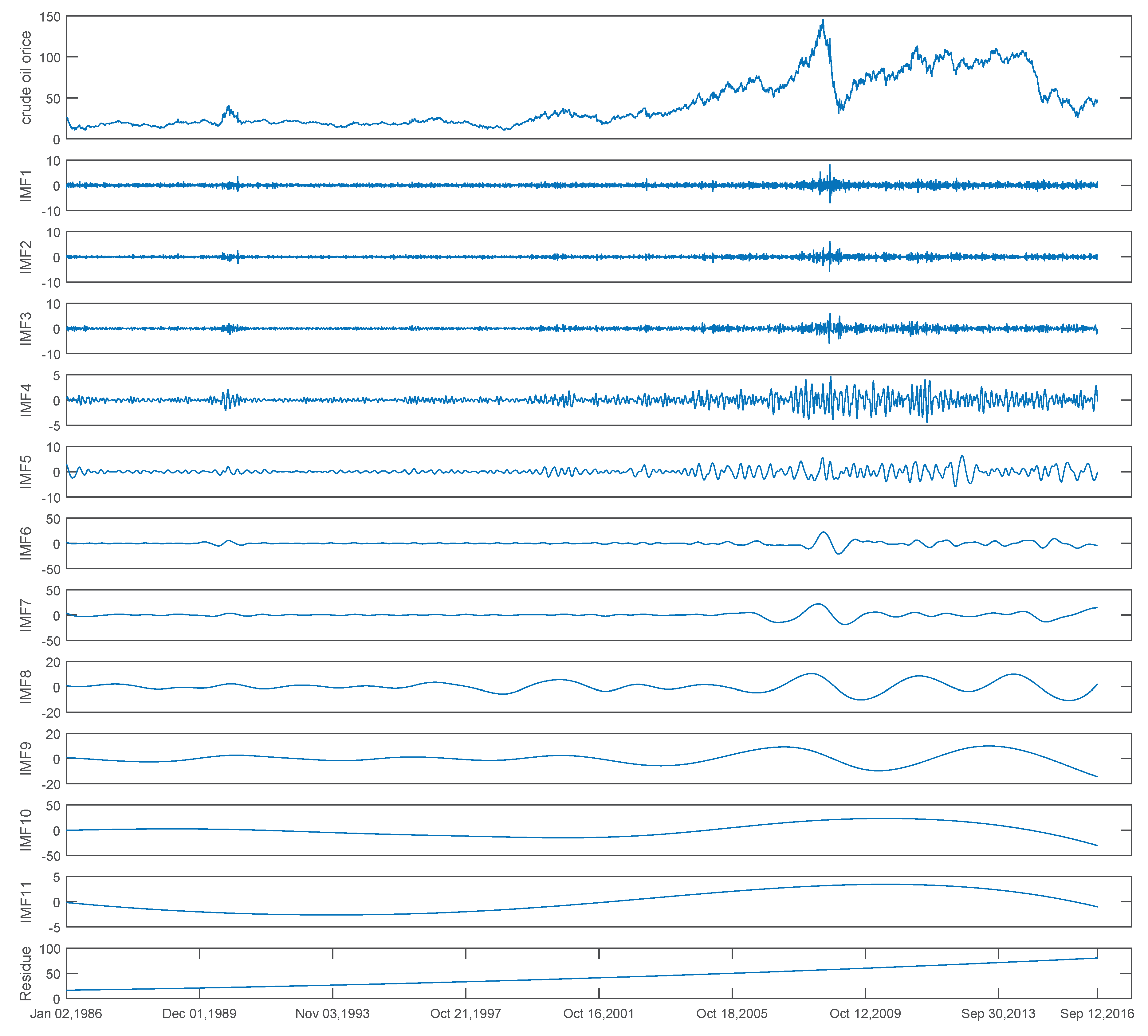
2.1. Ensemble Empirical Mode Decomposition

Ensemble empirical mode decomposition (EEMD) is an extended version of empirical mode decomposition (EMD) developed to overcome the drawback of the so-called “mode mixing” problem in the latter [30,56]. Contrary to traditional decomposition methodologies, EEMD is an empirical, direct, intuitive, and self-adaptive methodology that can decompose nonlinear and nonstationary time series into components (several IMFs and one residue), with each component having a length equal to the original signal. Since it was proposed, it has been widely applied to complex system analysis, showing its superiority in forecasting time series.

The main idea of EEMD is to perform EMD many times on the time series, given a number of Gaussian white noises to obtain a set of IMFs, and then the ensemble average of corresponding IMFs is treated as the final decomposed results. The main steps of EEMD are as follows:

Step 1:

Specify the number of ensemble M and the standard deviation of Gaussian white noises σ, with $i=0$;

Step 2:

$i=i+1$; Add a Gaussian white noise $n_i\left(t\right)$∼$N(0,{\sigma }^2)$ to crude oil price series $X\left(t\right)$ to construct a new series $X_i\left(t\right)$, as follows:

$$X_i\left(t\right)=X\left(t\right)+n_i\left(t\right).$$

(1)

Step 3:

Decompose $X_i\left(t\right)$ into m IMFs $c_{ij}\left(t\right)(j=1,\dots ,J)$ and a residue $r_i\left(t\right)$, as follows:

$$X_i\left(t\right)=\sum _{j=1}^m{c}_{ij}\left(t\right)+r_i\left(t\right),$$

(2)

where $c_{ij}$ is the j-th IMF in the i-th trial, and J is the number of IMFs, determined by the size of crude oil price series N with $J=\lfloor lo{g}_{2}N\rfloor -1$ [30].

Step 4:

If $i<M$, go to Step 2 to perform EMD again; otherwise, go to Step 5;

Step 5:

Calculate the average of corresponding IMFs of M trials as final IMFs:

$$c_j\left(t\right)=\frac{1}{M}\sum _{i=1}^M{c}_{ij}\left(t\right),i=1,\dots ,M;j=1,\dots ,J.$$

(3)

Once the EEMD completes, the original time series can be expressed as the sum of J IMFs and a residue, as follows:

$$X\left(t\right)=\sum _{j=1}^J{c}_j\left(t\right)+r_{J,t},$$

(4)

where $r_{J,t}$ is the final residue. Now, the issue of forecasting original time series becomes the new issue of forecasting each component decomposed by EEMD.

2.2. Particle Swarm Optimization

Particle swarm optimization (PSO)—firstly proposed by Eberhart and Kennedy—is an evolutionary computation algorithm that uses the velocity-displacement model through iteration to simulate swarm intelligence [57]. The algorithm initializes with a group of random particles in space of D dimensions, and each particle—representing a potential solution—is assigned a randomized velocity to change its position, searching for the optimal solution. In each iteration, the particles keep track of the local best solution $p_l$ and the global best solution $p_g$ to decide the flight speed and distance accordingly.

The ith particle has a position vector and a velocity vector in D dimensional space, described as $p_i=(p_{i1},p_{i2},\dots ,p_{iD})$ and $v_i=(v_{i1},v_{i2},\dots ,v_{iD})$, and the optimum locations achieved by the ith particle and population are also described as $p_{li}=(p_{li1},p_{li2},\dots ,p_{liD})$ and $p_g=(p_{g1},p_{g2},\dots ,p_{gD})$, respectively. The formulas to update the speed and position of the dth dimension of the ith particle are as follows, respectively:

$$v_{id}(t+1)=w{v}_{id}\left(t\right)+c_1{r}_1(p_{lid}-p_{id}\left(t\right))+c_2{r}_2(p_{gd}-p_{id}\left(t\right))$$

(5)

$$p_{id}(t+1)=p_{id}\left(t\right)+v_{id}(t+1))$$

(6)

where t is the current number of iteration, w is inertia weight, $c_1$ and $c_2$ are nonnegative accelerate constants, and $r_1$ and $r_2$ are random in the range of [0, 1].

PSO is good at real optimization. Therefore, in this research, we use PSO to optimize the weight and parameters in each single kernel for the combined kernel in RVM.

2.3. Relevance Vector Machine

Relevance vector machine (RVM)—put forward by Tipping [32]—can be applied to both regression and classification. Since forecasting crude oil price is related to regression, here we give a brief review of RVM for regression only. Readers can refer to [32] for more details on RVM.

Given a set of samples $\{x_i,t_i{\}}_{i=1}^N$, where $x_i\in R^d$ are d-dimensional vectors as inputs and $t_i\in R$ are real values as targets, and assuming that $t_i=y(x_i;w)+{ϵ}_i$ with ${ϵ}_i\sim N(0,{\sigma }^2)$, the RVM model for regression can be formulated as:

$$t=y(x;w)=\sum _{i=1}^N{w}_{i}K(x,x_i)+w_0,$$

(7)

where $K(x,x_i)$ is a kernel function on x and $x_i$, and $w_i$ is the weight of the kernel. Then, for a sample i, the conditional probability of the target is as follows:

$$p(t_i|x_i)=N(t_i|y(x_i;w),{\sigma }^2).$$

(8)

Assuming that the samples $\{x_i,t_i{\}}_{i=1}^N$ are independently generated, the likelihood of all the samples can be defined as follows:

$$\begin{array}{cc}p(t|w,{\sigma }^2)\hfill & =\prod _{i=1}^{N}N(t_i|y(x_i;w),{\sigma }^2)\hfill \\ & ={\left(2\pi {\sigma }^2\right)}^{-\frac{N}{2}}exp(-\frac{||t-{\mathsf{\Phi }w||}^2}{2{\sigma }^2}),\hfill \end{array}$$

(9)

where Φ is a design matrix having the size $N\times (N+1)$ with $\mathsf{\Phi }={[\varphi (x_1),\varphi (x_2),\dots ,\varphi (x_N)]}^T$, wherein each component is the vector of the response of kernel function associated with the sample $x_n$ as $\varphi \left(x_n\right)={[1,K(x_n,x_1),K(x_n,x_2),\dots ,K(x_n,x_N)]}^T$. It may cause over-fitting if we implement maximum-likelihood estimation for w and ${\sigma }^2$ directly, because the size of training samples is almost the same as the size of parameters. To overcome this, Tipping imposed a constraint on weights w from a Bayesian perspective, as follows [32]:

$$p(w|\alpha )=\prod _{i=0}^{N}N(w_i|0,{\alpha }_i^{-1}),$$

(10)

where α is an $N+1$ vector named hyperparameters. With the prior on weights, for all unknown samples, the posterior can be computed from the proceeds of Bayes inference as:

$$p(w,\alpha ,{\sigma }^2|t)=\frac{p(t|w,\alpha ,{\sigma }^2)\times p(w,\alpha ,{\sigma }^2)}{p\left(t\right)}.$$

(11)

For a given input point $x_{*}$, the predictive distribution of the corresponding target $t_{\ast }$ can be written as:

$$p(t_{\ast }|t)=\int p(t_{\ast }|w,\alpha ,{\sigma }^2)p(w,\alpha ,{\sigma }^2|t)dwd\alpha d{\sigma }^2.$$

(12)

It is difficult to directly compute the posterior $p(w,\alpha ,{\sigma }^2|t)$ in Equation (11). Instead, Tipping further decomposes it as follows:

$$p(w,\alpha ,{\sigma }^2|t)=p(w|t,\alpha ,{\sigma }^2)p(\alpha ,{\sigma }^2|t).$$

(13)

The computation of $p(w,\alpha ,{\sigma }^2|t)$ is now becoming the computation of two items: $p(w|t,\alpha ,{\sigma }^2)$ and $p(\alpha ,{\sigma }^2|t)$. The posterior distribution over weights can be written from Bayes’s rule:

$$\begin{array}{cc}p(w|t,\alpha ,{\sigma }^2)\hfill & =\frac{p(t|w,{\sigma }^2)p(w|\alpha )}{p(t|\alpha ,{\sigma }^2)}\hfill \\ & ={(2\pi {\sigma }^2)}^{-\frac{N+1}{2}}{|\sum |}^{-\frac{1}{2}}exp(-\frac{{(w-\mu )}^T{\sum }^{-1}(w-\mu )}{2}),\hfill \end{array}$$

(14)

where the posterior covariance and mean are as follows, respectively,

$$\sum ={(\beta {\mathsf{\Phi }}^T\mathsf{\Phi }+A)}^{-1},$$

(15)

$$\mu =\beta \sum {\mathsf{\Phi }}^{T}t,$$

(16)

with $\beta ={\sigma }^{-2}$ and $A=diag({\alpha }_0,{\alpha }_1,\dots ,{\alpha }_N)$, respectively.

As far as the second item at right hand side of Equation (13), it can be decomposed as:

$$p(\alpha ,{\sigma }^2|t)\propto p(t|\alpha ,{\sigma }^2)p(\alpha )p({\sigma }^2)\propto p(t|\alpha ,{\sigma }^2).$$

(17)

Therefore, the learning process of RVM is now transformed to maximizing Equation (18) with respect to the hyperparameters α and ${\sigma }^2$:

$$\begin{array}{cc}p(t|\alpha ,{\sigma }^2)\hfill & =\int p(t|w,{\sigma }^2)p(w|\alpha )dw\hfill \\ & ={\left(2\pi \right)}^{-\frac{N}{2}}{|{\sigma }^{2}I+\mathsf{\Phi }{A}^{-1}{\mathsf{\Phi }}^T|}^{-\frac{1}{2}}exp(-\frac{t^T{({\sigma }^{2}I+\mathsf{\Phi }{A}^{-1}{\mathsf{\Phi }}^T)}^{-1}t}{2}),\hfill \end{array}$$

(18)

where I is an identity matrix.

By simply setting the derivatives of Equation (18) to zero, we can obtain the re-estimation equations on α and ${\sigma }^2$ as follows, respectively:

$${\alpha }_i^{new}=\frac{1-{\alpha }_i{\sum }_{ii}}{{\mu }_i^2},$$

(19)

$${\left({\sigma }^2\right)}^{new}=\frac{||t-{\mathsf{\Phi }\mu ||}^2}{N-{\sum }_i(1-{\alpha }_i{\sum }_{ii})}.$$

(20)

With the iteration, the optimal values of α and ${\sigma }^2$—termed as ${\alpha }_{MP}$ and ${\sigma }_{MP}^2$ respectively—can be achieved by maximizing Equation (18).

Finally, for the given input point $t_{\ast }$, the predictive result can be computed as follows:

$$p(t_{\ast }|t,{\alpha }_{MP},{\sigma }_{MP}^2)=\int p(t_{\ast }|w,{\sigma }_{MP}^2)p(w|t,{\alpha }_{MP},{\sigma }_{MP}^2)dw=N(t_{\ast }|y_{\ast },{\sigma }_{\ast }^2),$$

(21)

where $y_{\ast }={\mu }^T\varphi \left(x_{\ast }\right)$ and ${\sigma }_{\ast }^2={\sigma }_{MP}^2+\varphi {\left(x_{\ast }\right)}^T\sum \varphi \left(x_{\ast }\right)$.

The kernel function in RVM plays a crucial role which significantly influences the performance of RVM. Therefore, it is important to select appropriate kernels according to the characteristics of the data instead of using a single fixed kernel. Some widely used single kernels include the linear kernel $K_{lin}(x_i,y_i)=x_i^T{y}_i$, the polynomial kernel $K_{poly}(x_i,y_i)={(a(x_i^T{y}_i)+b)}^c$, the RBF kernel $K_{rbf}(x_i,y_i)=exp(-\frac{||x_i-y_i{||}^2}{2d})$ (here we use d to represent ${\sigma }^2$ for short), and the sigmoid kernel $K_{sig}(x_i,y_i)=tanh(e(x_i^T{y}_i)+f)$. Among the kernels, the parameters $a-f$ usually need to be specified by users. In this paper, we integrate the above-mentioned four kernels into a combined kernel for RVM, which can be represented as:

$$K_{comb}(x_i,y_i)={\lambda }_1{K}_{lin}(x_i,y_i)+{\lambda }_2{K}_{poly}(x_i,y_i)+{\lambda }_3{K}_{rbf}(x_i,y_i)+{\lambda }_4{K}_{sig}(x_i,y_i),$$

(22)

where ${\lambda }_1$–${\lambda }_4$ are the weights for the four kernels that satisfy ${\sum }_{i=1}^4{\lambda }_i=1$. In this way, each single kernel of the four kernels is a special case of the combined kernel. For example, when ${\lambda }_1={\lambda }_2={\lambda }_4=0$ and ${\lambda }_3=1$, the combined kernel degenerates to the RBF kernel. In the combined kernel, ten parameters (${\lambda }_1$, ${\lambda }_2$, ${\lambda }_3$, ${\lambda }_4$, a, b, c, d, e, and f) need to be optimized.

2.4. Adaptive PSO for Parameter Optimization in RVM

For a specific problem, it is hard to set appropriate values for the parameters in the combined kernel in Equation (22) according to priori knowledge. PSO is a widely used real optimization algorithm that could be used in this case. However, in traditional PSO, the inertia weight for each particle in one generation is fixed, and it varies with the iteration—ignoring the difference among particles. Some varieties of PSO adaptively adjust the inertia wight of each particle based on one or more feedback parameters [58]. Ideally, the particles far from the global best particle should have larger inertia weight with more exploration ability, while the ones close to the global best particle should have smaller inertia weight with more exploitation ability. To cope with this issue, in this paper, an adaptive PSO (APSO) is proposed to optimize the parameters in RVM, which adaptively adjusts the inertia weight of each particle in an iteration according to the distance between the current particle and the global best particle.

Definition 1.

Distance between two particles. The distance between two particles $p_i$ and $p_j$ can be defined as:

$$dist(p_i,p_j)=\sqrt{\sum _{k=1}^d{(p_{ik}-p_{jk})}^2+{(f\left(p_i\right)-f\left(p_j\right))}^2},$$

(23)

where d is the dimension of particle, and f is the fitness function. It is worth noting that each dimension in Equation (23) needs to be mapped into the same scale (e.g., [0,1]) in order for the computation to make sense. According to this definition, the distance between two particles has three properties: (1) $dist(p_i,p_j)=dist(p_j,p_i)$; (2) $dist(p_i,p_i)=0$; (3) $dist(p_i,p_k)+dist(p_k,p_j)\ge dist(p_i,p_j)$.

Definition 2.

Average distance of population. The average distance of the population can be defined as:

$$mdist=\frac{2{\displaystyle \sum _{i=1}^N}{\displaystyle \sum _{j=1}^{i-1}}dist(p_i,p_j)}{N(N-1)},$$

(24)

where N is the total number of particles in a swarm.

In this paper, we propose an adaptive strategy to adjust the inertia weight for one particle $p_i$ in the t-th iteration by Equation (25):

$$w_{t,i}=\left\{\begin{array}{cc}{w}_{min}+\frac{w_{max}-w_{min}}{T}t,\hfill & dist(p_i,p_g)>mdist\hfill \\ w_{min}+\frac{w_{max}-w_{min}}{mdist}dist(p_i,p_g),\hfill & dist(p_i,p_g)\le mdist\hfill \end{array}\right.,$$

(25)

where T is the number of total iterations, $p_g$ is the global best particle, and $w_{max}$ and $w_{min}$ are the maximal and minimal inertia weights specified by users, respectively. The main idea of Equation (25) is to adjust the inertia weight of each particle adaptively according to its distance from the global best particle. If the current particle is far from the global best particle, it uses traditional inertia weight. Otherwise, it adaptively adjusts its inertia weight according to its distance to the global best particle.

The model using APSO to optimize the parameters of the combined kernel in RVM—called APSO-RVM—can be presented as:

Step 1:

Setting parameters. Set the following parameters for running APSO, population size P, maximal iteration times T, the maximal and minimal inertia weights $w_{max}$ and $w_{min}$, the range of the ten parameters to be optimized;

Step 2:

Encoding. Encode the ten parameters into a particle (vector) $p_i=(p_{i1},p_{i2},\dots ,p_{i10})$ to represent ${\lambda }_1$, ${\lambda }_2$, ${\lambda }_3$, ${\lambda }_4$, a, b, c, d, e, and f accordingly;

Step 3:

Defining the fitness function. The fitness function is defined by root mean square error (RMSE):

$$f\left(p_i\right)=\sqrt{\frac{1}{N}\sum _{n=1}^N{(y_i-\varphi (x_i,p_i))}^2},$$

(26)

where N is the size of training samples, $y_i$ is the true target of the input $x_i$, and $\varphi (x_i,p_i)$ is the predicted target associated with $x_i$ and the parameter $p_i$;

Step 4:

Initializing. Set $t=0$; randomly generate initial speed and position for each particle; use the value of particle $p_i$ to compose the kernel for RVM in Equation (22), and then evaluate each particle; $p_i$ is selected as $p_{li}$, while the particle with the optimal fitness is selected as $p_g$;

Step 5:

Updating speed and position. Set $t=t+1$; calculate the inertia weight using Equation (25), and update the speed and position according to Equations (5) and (6), respectively;

Step 6:

Evaluating particles. Evaluate each particle by fitness function;

Step 7:

Updating the historical best particle, if necessary. If $f\left(p_i\right)\le f\left(p_{li}\right)$, then $p_{li}=p_i$;

Step 8:

Updating the global best particle, if necessary. If $f\left(p_i\right)\le f\left(p_g\right)$, then $p_g=p_i$;

Step 9:

Judging whether the iteration terminates or not. If $t\le T$, go to Step 5. Otherwise, stop the iteration and output $p_{gb}$ as the optimized parameters for the combined kernel in RVM. The optimal RVM predictor is obtained at this point.

The APSO is based on the framework of PSO, and the main improvement lies in that each particle has its own inertia weight according to its distance from the global best particle. In this paper, the APSO is applied to adaptively searching the optimal weights and parameters of the single kernels for the combined kernel in RVM to predict crude oil price.

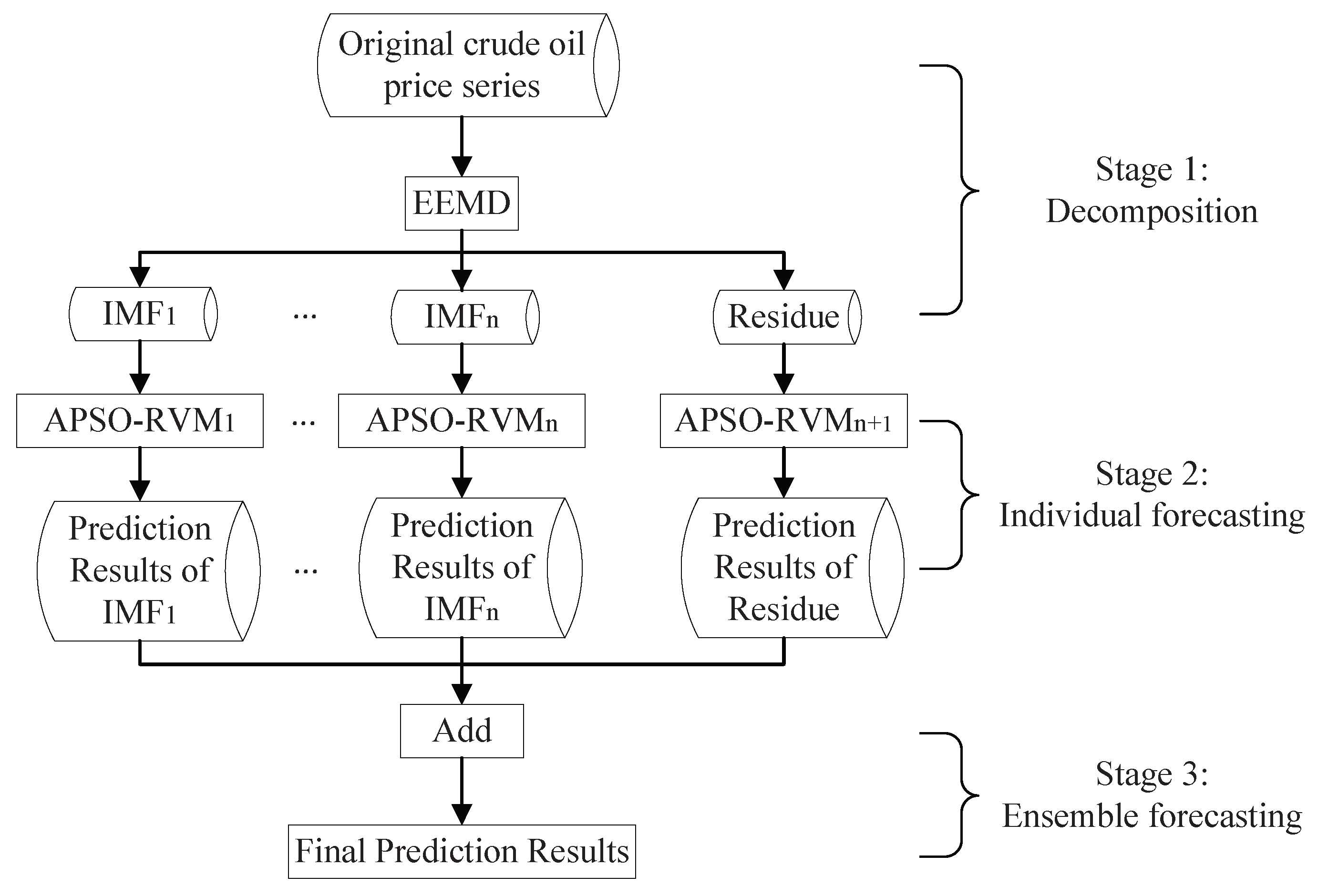
2.5. The Proposed EEMD–APSO–RVM Model

Following the framework of “decomposition and ensemble”, a three-stage methodology that integrates ensemble empirical mode decomposition (EEMD), adaptive particle swarm optimization (APSO), and relevance vector machine (RVM)—termed EEMD-APSO-RVM—can be formulated for forecasting crude oil price. As shown in Figure 1, the proposed EEMD-APSO-RVM generally consists of three main stages:

Stage 1:

Decomposition. The original crude oil price series $x_t,(t=1,2,\dots ,T)$ is decomposed into with $J=\lfloor lo{g}_{2}T\rfloor -1$ intrinsic mode function (IMF) components $c_{j,t},(j=1,2,\dots ,J)$ and one residue component $r_{N,t}$ using EEMD;

Stage 2:

Individual forecasting. RVM with the combined kernel optimized by APSO is used to forecast each component in Stage 1 independently, resulting in the predicted values of IMFs ${\widehat{c}}_{j,t}$ and that of the residue ${\widehat{r}}_{N,t}$, respectively;

Stage 3:

Ensemble forecasting. The final predicted results ${\widehat{x}}_t$ can be obtained by simply adding the predicted results of all IMF components and the residue; i.e., ${\widehat{x}}_t={\displaystyle \sum _{j=1}^J}{\widehat{c}}_{j,t}+{\widehat{r}}_{N,t}$.

The proposed EEMD-APSO-RVM is one of the typical strategies of “divide and conquer”. The complicated question of forecasting the original crude oil price is transformed to several questions of forecasting relatively simple components independently. The EEMD-APSO-RVM adopts a combined kernel that integrates four commonly used kernels. Furthermore, the weights and parameters in the combined kernel are adaptively optimized by an extension of PSO. The EEMD-APSO-RVM decomposes the crude oil price into several IMFs and one residue for forecasting individually, instead of using the nonlinear and nonstationary raw data as the input to a single forecasting method; this can improve the forecasting accuracy, because the individual forecasting is a relatively easy task. The kernel-trick RVM has the ability to accurately predict time series such as wind speed and electricity price, which will benefit crude oil price forecasting. The APSO adaptively optimizes the parameters in the kernel, trying to find the optimal kernel to improve the forecasting results. All these attributes make it possible for the EEMD-APSO-RVM to improve the accuracy of crude oil price forecasting.

3. Numerical Example

To demonstrate the performance of the proposed EEMD-APSO-RVM, in this paper, we select the crude oil price of West Texas Intermediate (WTI) as experimental data, as described in Section 3.1. The evaluation criteria are introduced in Section 3.2. Section 3.3 gives the parameter settings and data preprocessing for the experiments, and in Section 3.4, the experimental results are reported. We further analyse the robustness and running time of the proposed method in Section 3.5. Finally, some interesting findings can be obtained from the experimental study.

3.1. Data Description

The crude oil price of WTI can be accessed from the US energy information administration (EIA) [59]. We use the daily close price covering the period of 2 January 1986 to 12 September 2016, with 7743 observations in total for experiments. Among the observations, the first 6194 from 2 January 1986 to 21 July 2010 are treated as training samples, while the remaining 1549 from 22 July 2010 to 12 September 2016 are for testing—accounting for 80% and 20% of total observations, respectively.

We conduct h-step-ahead predictions with horizon $h=1,3,6$ in this study. Given a time series $x_t,(t=1,2,\dots ,T)$, the h-step-ahead prediction for $x_{t+h}$ can be formulated as:

$${\widehat{x}}_{t+h}=f(x_{t-(l-1)},x_{t-(l-2)},\dots ,x_{t-1},x_t),$$

(27)

where ${\widehat{x}}_{t+h}$ is the h-step-ahead predicted value at time t, $x_t$ is the true value at time t, and l is the lag orders.

3.2. Evaluation Criteria

The root mean squared error (RMSE), the mean absolute percent error (MAPE), and the directional statistic ($D_{stat}$) are selected to evaluate the performance of the proposed method. With the true value $x_t$ and the predicted value ${\widehat{x}}_t$ at time t, RMSE is defined as:

$$RMSE=\sqrt{\frac{1}{N}\sum _{t=1}^N{(x_t-{\widehat{x}}_t)}^2},$$

(28)

where N is the number of testing observations. Note that the RMSE here has the same meaning as Equation (26), where the predicted value is represented by $\varphi (x_i,p_i)$.

As another evaluation criteria for prediction accuracy, MAPE is defined as:

$$MAPE=\frac{1}{N}\sum _{t=1}^N|\frac{x_t-{\widehat{x}}_t}{x_t}|.$$

(29)

In addition, Dstat measures the ability to forecast the direction of price movement, which is defined as:

$$D_{stat}=\frac{1}{N}\sum _{t=1}^N{\alpha }_t\times 100\%,$$

(30)

where ${\alpha }_t=0$ if $({\widehat{x}}_{t+1}-x_t)(x_{t+1}-x_t)<0$; otherwise, ${\alpha }_t=1$.

An ideal forecasting method should achieve low RMSE, low MAPE, and high $D_{stat}$.

3.3. Experimental Settings

In order to evaluate the performance of the proposed methods, some state-of-the-art models were selected as benchmarks to compare with the EEMD-APSO-RVM. In the decomposition stage, we select EMD as a benchmark. In the prediction stage, the compared models include one classical statistical method (ARIMA) and two popular AI models (LSSVR and ANN). In addition, RVM with a single kernel (RVMlin, RVMpoly, RVMrbf, RVMsig) and RVM with a combined kernel from the former four single kernels optimized by standard PSO (PSO-RVM) are also independently employed in this stage. Therefore, we have eight single methods (PSO-RVM, RVMlin, RVMpoly, RVMrbf, RVMsig, ANN, LSSVR, and ARIMA) to compare with APSO-RVM, and fifteen ensemble methods (EEMD-PSO-RVM, EEMD-RVMlin, EEMD-RVMpoly, EEMD-RVMrbf, EEMD-RVMsig, EEMD-ANN, EEMD-LSSVR, EMD-PSO-RVM, EMD-APSO-RVM, EMD-RVMlin, EMD-RVMpoly, EMD-RVMrbf, EMD-RVMsig, EMD-ANN, and EMD-LSSVR) to compare with EEMD-APSO-RVM. All methods are shown in

Table 1. Descriptions of all the methods in the experiments. ANN: artificial neural network; PSO: particle swarm optimization.

Type	Name	Descriptions
		Decomposition	Forecasting	Ensemble
Single	APSO-RVM	-	RVM with a combined kernel optimized by APSO	-
	PSO-RVM	-	RVM with a combined kernel optimized by standard PSO	-
	RVMlin	-	RVM with a linear kernel	-
	RVMpoly	-	RVM with a polynomial kernel	-
	RVMrbf	-	RVM with a radial basic function kernel	-
	RVMsig	-	RVM with a sigmoid kernel	-
	ANN	-	Back propagation neural network	-
	LSSVR	-	Least squares support vector regression	-
	ARIMA	-	Autoregressive integrated moving average	-
Ensemble	EEMD-APSO-RVM	EEMD	RVM with a combined kernel optimized by APSO	Addition
	EEMD-PSO-RVM	EEMD	RVM with a combined kernel optimized by standard PSO	Addition
	EEMD-RVMlin	EEMD	RVM with a linear kernel	Addition
	EEMD-RVMpoly	EEMD	RVM with a polynomial kernel	Addition
	EEMD-RVMrbf	EEMD	RVM with a radial basic function kernel	Addition
	EEMD-RVMsig	EEMD	RVM with a sigmoid kernel	Addition
	EEMD-ANN	EEMD	Back propagation neural network	Addition
	EEMD-LSSVR	EEMD	Least squares support vector regression	Addition
	EMD-APSO-RVM	EMD	RVM with a combined kernel optimized by APSO	Addition
	EMD-PSO-RVM	EMD	RVM with a combined kernel optimized by standard PSO	Addition
	EMD-RVMlin	EMD	RVM with a linear kernel	Addition
	EMD-RVMpoly	EMD	RVM with a polynomial kernel	Addition
	EMD-RVMrbf	EMD	RVM with a radial basic function kernel	Addition
	EMD-RVMsig	EMD	RVM with a sigmoid kernel	Addition
	EMD-ANN	EMD	Back propagation neural network	Addition
	EMD-LSSVR	EMD	Least squares support vector regression	Addition

.

The parameters for APSO are listed in

Table 2. Parameters for APSO.

Description	Symbol	Range / Value
Population size	P	20
Maximal iterations	T	40
Particle dimension	D	10
Maximal, minimal inertia weight	$w_{max},w_{min}$	0.9, 0.4
Accelerate constants	$c_1,c_2$	1.49, 1.49
Kernel weight	${\lambda }_1,{\lambda }_2,{\lambda }_3,{\lambda }_4$	[0, 1]
Coefficient in Kpoly	a	[0, 2]
Constant in Kpoly	b	[0, 10]
Exponent in Kpoly	c	[1, 4]
Width in Krbf	d	[$2^{-4},2^{12}$]
Coefficient in Ksig	e	[0, 4]
Constant in Ksig	f	[0, 8]

. The standard PSO uses the same parameters as APSO. Note that to guarantee ${\sum }_{i=1}^4{\lambda }_i=1$, we simply map the values in particles to new values to be applied to the combined kernel with ${\lambda }_j^{\prime }=\frac{{\lambda }_j}{{\sum }_{i=1}^4{\lambda }_i}$. For b, we use $b=round\left(b\right)$ to get an integer as the exponent. Following some previous work [4,27], we apply RBF kernel in LSSVR and use grid search to find the optimal γ and ${\sigma }^2$ in the range of {$2^k,k=-4,-3,\dots ,12$} and {$2^k,k=-4,-3,\dots ,12$}, respectively. For ANN, we use a back propagation neural network and set ten as the number of hidden nodes. The iteration times of ANN was set to 10,000. For the parameters in single RVM-related predictors (i.e., $a-f$), we search the best parameters in the same ranges as those in APSO (listed in Table 2) with an interval of 0.2, excepting that c varies with an interval of 1 and d varies in {$2^k,k=-4,-3,\dots ,12$}. We use the Akaike information criterion (AIC) [60] to determine the ARIMA parameters (p-d-q). We also set the lag orders in Equation (27) to six, as analysed in [61].

Regarding ensemble models, we firstly add white noise with a standard deviation of 0.15 to the original crude oil price, and then set 100 as the number of ensembles in EEMD. The decomposition results of the original crude oil price by EEMD is shown in Figure 2, with 11 IMFs and one residue.

To set up the stage for a fair comparison, we applied the Min–Max Normalization (as shown in Equation (31)) for all of the data:

$$x_{norm}=(x-x_{min})/(x_{max}-x_{min}),$$

(31)

where $x_{min}$ and $x_{max}$ are the minimal and maximal values for one dimension in data, respectively, and $x_{norm}$ and x are the normalized and the original values, respectively. It is clear that the normalization maps the original values to the range $[0,1]$. Conversely, after obtaining the predicted value from the normalized data ${\widehat{x}}_{norm}$, the corresponding expected predicted value $\widehat{x}$ in original scale can be computed as:

$$\widehat{x}=x_{min}+(x_{max}-x_{min})\ast {\widehat{x}}_{norm}.$$

(32)

All of the experiments were conducted by Matlab 8.6 (Mathworks, Natick, MA, USA) on a 64-bit Windows 7 (Microsoft, Redmond, WA, USA) with 32 GB memory and 3.4 GHz I7 CPU.

3.4. Results and Analysis

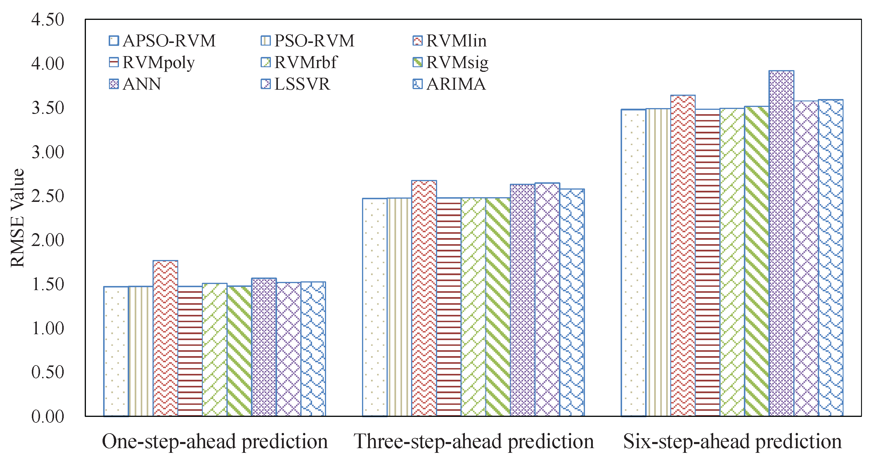
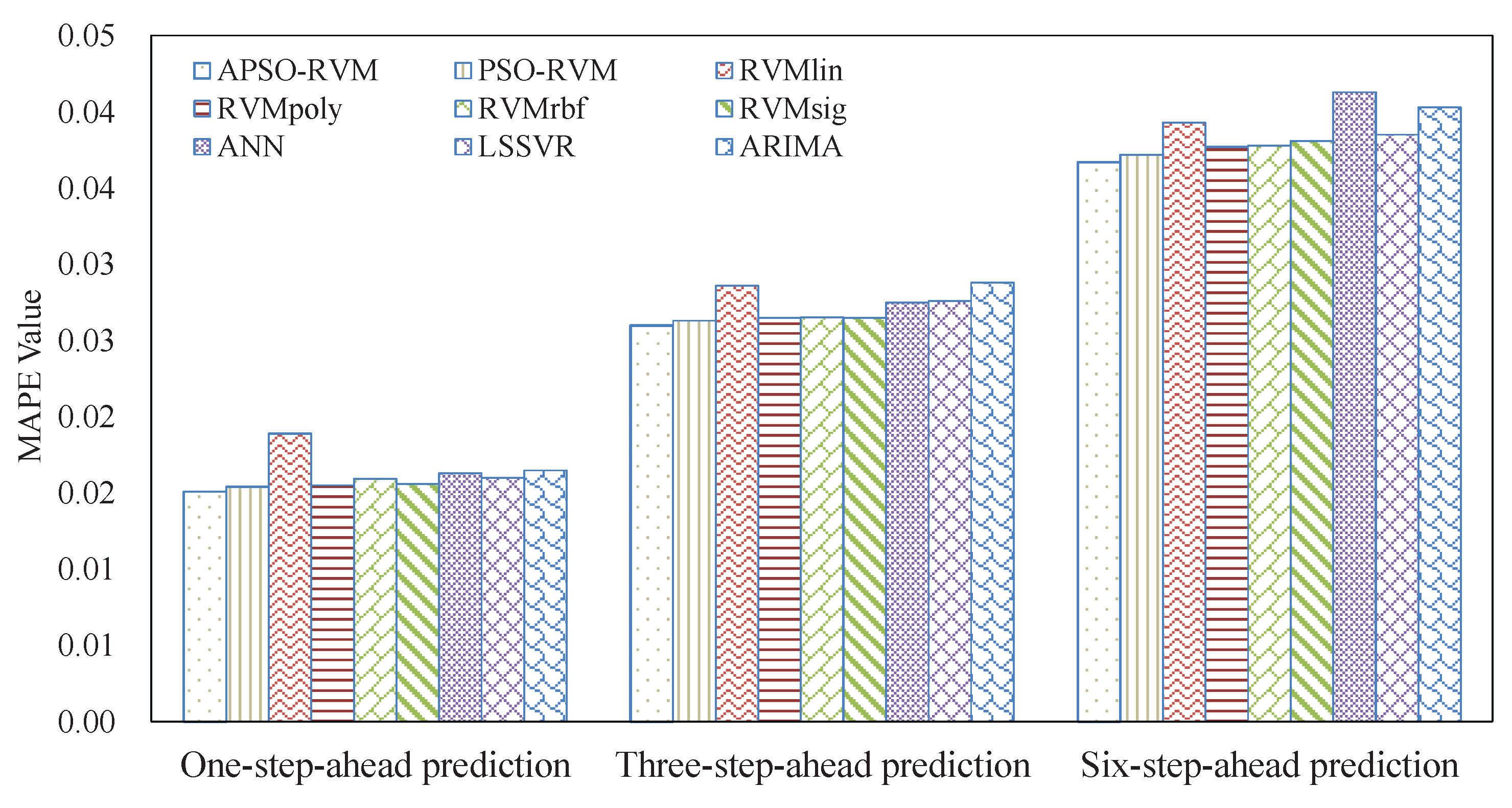
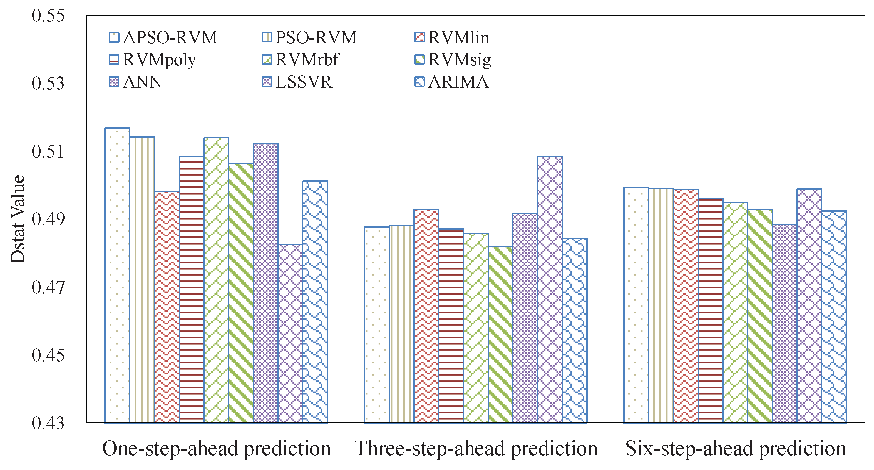
3.4.1. Results of Single Models

We firstly evaluate the single models (i.e., APSO-RVM, PSO-RVM, RVMlin, RVMpoly, RVMrbf, RVMsig, ANN, LSSVR, and ARIMA) in terms of MAPE, RMSE, and Dstat, as shown in Figure 3, Figure 4 and Figure 5. From these results, it can be concluded that the proposed APSO-RVM might be the most powerful single model among all the single models in forecasting crude oil price.

The MAPE value by the APSO-RVM is the lowest amongst the nine single models at all horizons, followed by PSO-RVM, RVMpoly, RVMrbf, and RVMsig. The performances of the latter four models are quite alike, except that the MAPE value by RVMrbf at horizon one is slightly high. RVMlin achieves the highest values at horizon one and horizon three, and the third highest value at horizon six, showing its poor performance in forecasting crude oil price. The possible reason for this is that the crude oil price data is not linearly separable. The results by the state-of-the-art AI benchmark models (ANN and LSSVR) are very close at horizon one and horizon three. However, LSSVR outperforms ANN at horizon six. The statistical model—ARIMA—ranks sixth in all cases. This is probably because, as a typical linear model, it is difficult for ARIMA to accurately forecast crude oil price due, to its nonlinearity and nonstationarity.

As far as RMSE, the prediction accuracy of APSO-RVM is still ranked first among all of the compared benchmark models in all cases, although it is very close to the corresponding result by PSO-RVM. For the RVM model with a single kernel, RVMpoly, RVMrbf, and RVMsig achieve very close results, which are slightly higher than that of APSO-RVM, followed by RVMlin with the poorest results at horizon one and horizon three, and the second poorest result at horizon six among all methods. ANN, LSSVR, and ARIMA achieve very similar RMSE values at each horizon, except ANN underperforms LSSVR and ARIMA at horizon six.

From the perspective of directional accuracy, all of the models produce quite similar results, ranging from 0.48 to 0.52. It can be easily seen that none of the models can be proven to be better than the others. In spite of its leading performance in terms of MAPE and RMSE, APSO-RVM does not significantly outperform other models at all horizons regarding Dstat. The APSO-RVM ranks first at horizon one, fifth at horizon three, and first with slight advantages at horizon six. It is interesting that LSSVR ranks first at horizon three and second at horizon six, but it ranks last at horizon one. Another interesting finding is that the values of seven out of nine models at horizon six are higher than those at horizon three. Therefore, the performance of single models is not stable when forecasting the direction of crude oil price.

From the results by single models, it can be seen that none of the methods can consistently outperform others in all cases in terms of MAPE, RMSE, and Dstat. Another interesting finding is that many methods achieve very close results in most cases, although the APSO-RVM is better than others in eight out of nine cases. In addition, all of the results by the methods are undesirable, even for the best result. For example, the results of Dstat by all methods were between 0.48 and 0.52, which tends to guessing randomly, making it unpractical. All of these findings show that it is a difficult task to accurately forecast crude oil price using the nonlinear and nonstationary raw price. The main reason might be that the single models have their limitations in achieving high accuracy because of the complexity of crude oil price. Hence, in this work, we develop a novel “decomposition and ensemble” method to improve the performance of single models in forecasting crude oil price.

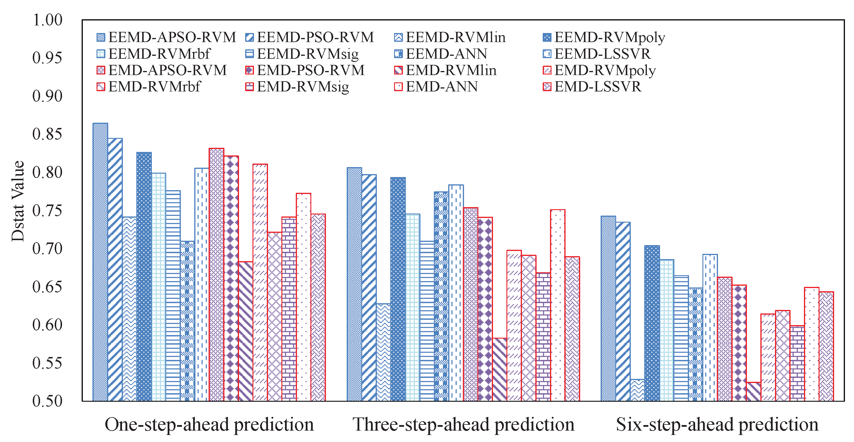
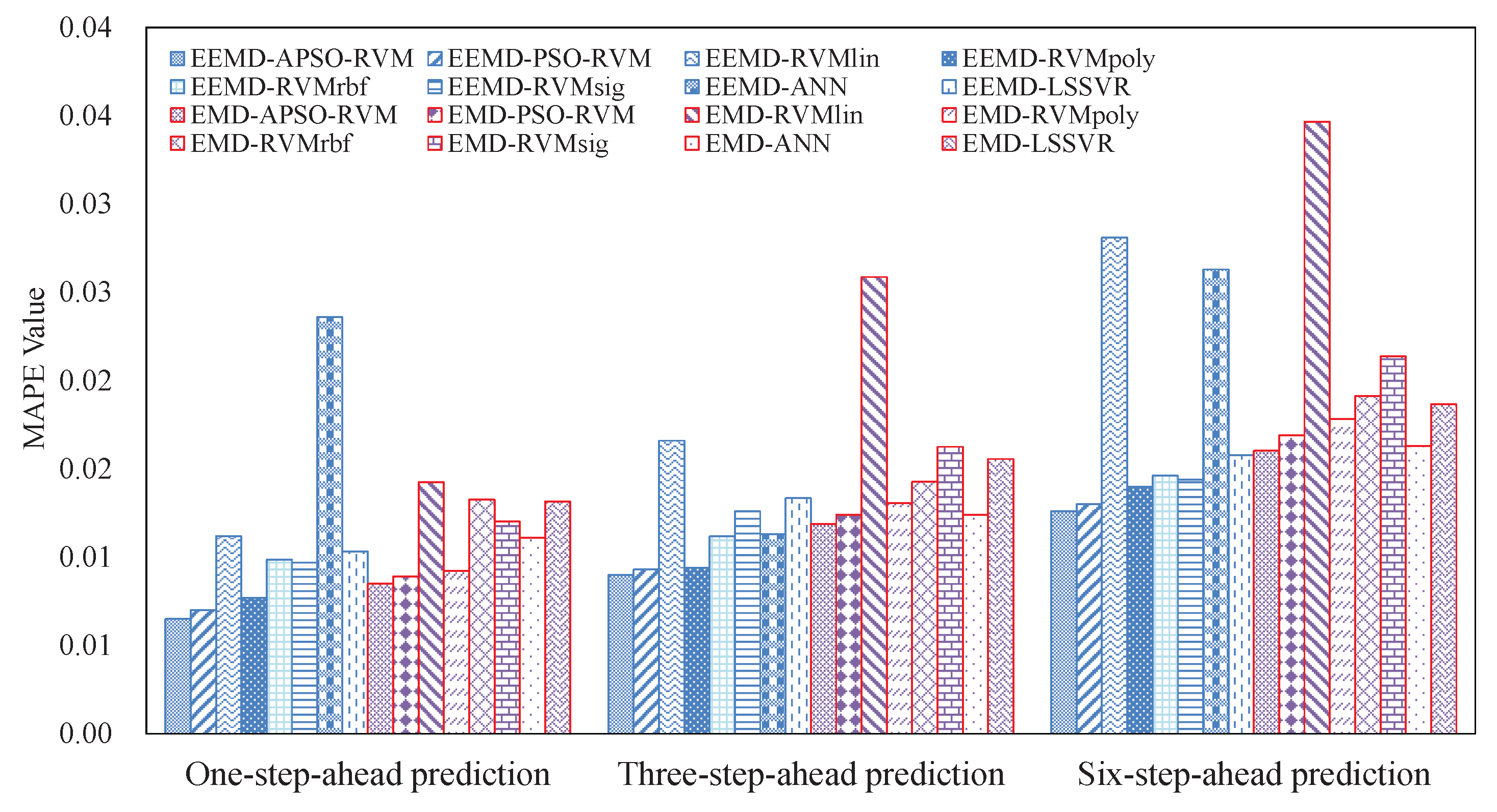
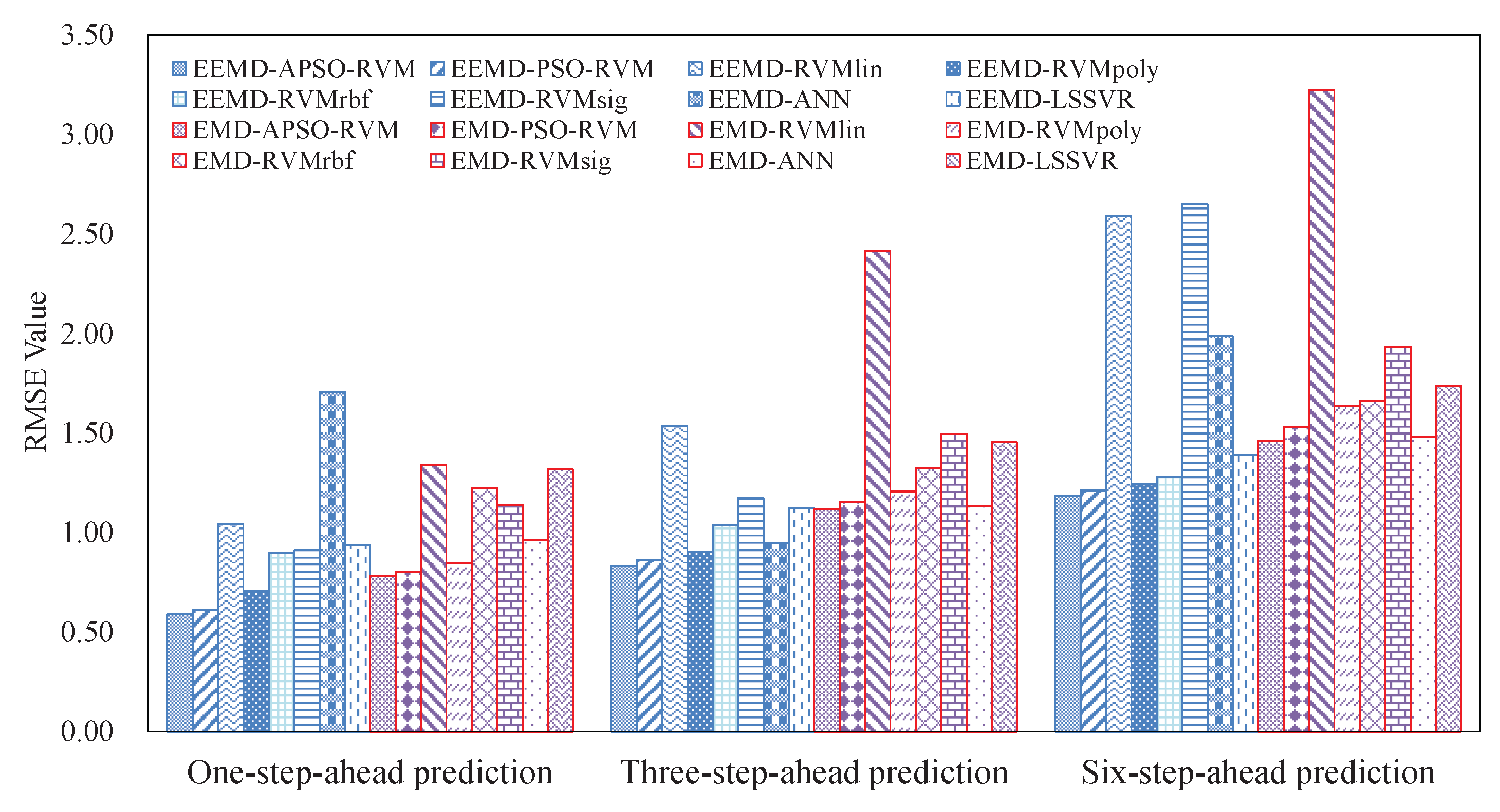
3.4.2. Results of Ensemble Models

Regarding the ensemble models (i.e., EEMD-APSO-RVM, EEMD-PSO-RVM, EEMD-RVMlin, EEMD-RVMpoly, EEMD-RVMrbf, EEMD-RVMsig, EEMD-ANN, EEMD-LSSVR, EMD-APSO-RVM, EMD-PSO-RVM, EMD-RVMlin, EMD-RVMpoly, EMD-RVMrbf, EMD-RVMsig, EMD-ANN, and EMD-LSSVR), Figure 6, Figure 7 and Figure 8 show the corresponding results in terms of MAPE, RMSE, and Dstat. From these results, it can be easily seen that the proposed EEMD-APSO-RVM is the best model that achieves the lowest MAPE value, the lowest RMSE value, and the highest Dstat value at each horizon.

At each horizon, the MAPE value of EEMD-APSO-RVM ranks first among all models, being far lower than that of many other ensemble models. At the same time, the MAPE value of EMD-APSO-RVM also ranks first among all of the EMD-related methods. It shows the superiority of APSO-RVM in forecasting crude oil price. Accordingly, the EEMD-PSO-RVM and the EMD-PSO-RVM rank the second among EEMD-related and EMD-related methods, respectively, at each horizon, with slightly worse results than those of counterpart EEMD-APSO-RVM and EMD-APSO-RVM. EEMD-RVMpoly ranks third in terms of MAPE at each horizon, and EEMD-RVMsig and EEMD-RVMrbf are slightly worse than EEMD-RVMpoly, but are still better than many other methods. Among the EEMD-RVM family methods, EEMD-RVMlin is the poorest model, and it always ranks last at three horizons when compared with other EEMD-RVM-related models. It is clear that RVM with a combined kernel outperforms RVMs with a single kernel. Regarding ANN and LSSVR, it is interesting that ANN underperforms LSSVR twice with EEMD, while the first always outperforms the latter with EMD. For these two AI models, it is difficult to judge which is superior to the other, since they are both parameter-sensitive and it is difficult for traditional methods to find their optimal parameters. From the perspective of decomposition algorithms, it can be found that the ensemble methods with EEMD as decomposition method are much better than their counterpart methods with EMD, except for ANN at horizon one and horizon six, showing that the EEMD is a more effective decomposition method in time series analysis. Furthermore, EEMD-APSO-RVM significantly decreases the MAPE values when compared with the single APSO-RVM method, demonstrating the effectiveness of the decomposition method for forecasting performance.

Focusing on the RMSE values (shown in Figure 7), findings similar to those of MAPE can be obtained. EEMD-APSO-RVM still ranks first amongst all benchmark models, with 0.59, 0.83, and 1.18 at horizon one, horizon three, and horizon six, respectively. The results of EEMD-APSO-RVM are far less than those by any other models, except EEMD-PSO-RVM has slightly worse results at corresponding horizons. This further confirms that the proposed EEMD-APSO-RVM is effective for forecasting crude oil price. Most ensemble methods obviously outperform their corresponding single method. This is mainly attributed to the fact that EMD or EEMD can remarkably improve the prediction power of the models. Generally speaking, the ensemble methods with EEMD have better results than their corresponding methods with EMD, due to the good performance of EEMD on data analysis.

As far as Dstat (shown in Figure 8), all the values by ensemble models are higher than 0.525, and are quite different from the results of single models (as shown in Figure 5), where the highest value is less than 0.520. This demonstrates that the “decomposition and ensemble” framework can notably improve the performance of directional prediction. At each horizon, the proposed EEMD-APSO-RVM achieves the highest Dstat value (0.86, 0.81, and 0.74 at horizon one, horizon three, and horizon six, respectively), showing its superiority over all other methods. Similarly, EMD-APSO-RVM also outperforms all other EMD-related models at each horizon. The poorest results were usually achieved by RVM models with linear kernel, except that the EEMD-RVMlin obtains the second poorest value at horizon one, further demonstrating that the components from crude oil price are not linearly separable.

3.5. Analysis of Robustness and Running Time

Although EEMD-APSO-RVM succeeds in forecasting crude oil price, it has disadvantages. First, since the PSO uses many random values in the evolutionary process, it is hard for it to reproduce the experiments with the exact solutions. Second, it is time-consuming for the EEMD-APSO-RVM to find the optimal parameters and to compute the combined kernel.

To evaluate the robustness and stableness of the proposed EEMD-APSO-RVM, we repeated the experiments 10 times and report the results in terms of means and standard deviations (std.) of MAPE, RMSE, and Dstat in

Table 3. Statistical results of running the experiment ten times by the EEMD-APSO-RVM (mean ± std.).

Horizon	MAPE	RMSE	Dstat
One	0.0065 ± 0.0001	0.5905 ± 0.0110	0.8643 ± 0.0032
Three	0.0091 ± 0.0001	0.8324 ± 0.0340	0.8062 ± 0.0037
Six	0.0126 ± 0.0003	1.1843 ± 0.0702	0.7028 ± 0.0028

. It can be seen that the standard deviations of MAPE and Dstat are far less than 0.01, and at the same time, the standard deviation in each case is lower than 5% of corresponding mean. For RMSE, the standard deviations are slightly higher than those of MAPE and Dstat. However, even the poorest standard deviation in terms of RMSE is still less than 6% of the corresponding mean. The results show that EEMD-APSO-RVM is quite stable and robust for forecasting crude oil price.

In the training phase of the EEMD-APSO-RVM, to find the optimal parameters for the combined kernel, many particles need to be evaluated by fitness function, which is time-consuming. It takes about 10 h to train a model at one horizon in our experimental environment (Matlab 8.6 on a 64-bit Windows 7 with 32 GB memory and 3.4 GHz I7 CPU), while it takes only about 3 s to test the 1549 samples with the optimized parameters. In practice, the testing time plays a more important role than the training time, because the training phase is usually completed with off-line data and it runs only once. Therefore, the time consumed by the EEMD–APSO–RVM is acceptable.

3.6. Summarizations

From the above discussions, some interesting findings can be obtained, as follows:

(1)

Due to nonlinearity and nonstationarity, it is difficult for single models to accurately forecast crude oil price.

(2)

The RVM has a good ability to forecast crude oil price. Even with a single kernel, SVM may outperform LSSVM, ANN, and ARIMA in many cases.

(3)

The combined kernel can further improve the accuracy of RVM. PSO can be applied to optimize the weights and parameters of the single kernels for the combined kernel in RVM. In this case, the proposed APSO outperforms the traditional PSO.

(4)

The EEMD-related methods achieve better results than the counterpart EMD-related methods, showing that EEMD is more suitable for decomposing crude oil price.

(5)

With the benefits of EEMD, APSO, and RVM, the proposed ensemble EEMD–APSO–RVM significantly outperforms any other compared models listed in this paper in terms of MAPE, RMSE, and Dstat. At the same time, it is a stable and effective forecasting method in terms of robustness and running time. These all show that the EEMD–APSO–RVM is promising for crude oil price forecasting.

4. Conclusions

This paper proposes a novel model integrating EEMD, adaptive PSO, and RVM (namely EEMD-APSO-RVM) for forecasting crude oil price based on the “decomposition and ensemble” framework. In the decomposition phase, we used EEMD to decompose the raw crude oil price into components of several IMFs and one residue. In the single forecasting phase, we utilized RVM with a combined kernel optimized by an adaptive PSO to forecast each component individually. Finally, the predicted results of all components were aggregated by simple addition. To validate the EEMD-APSO-RVM, eight other single benchmark models and fifteen ensemble models were employed to compare the forecasting results of the crude oil spot price of WTI at three different horizons in terms of MAPE, RMSE, and Dstat. To the best of our knowledge, it is the first time that RVM with combined kernels have been applied to forecasting crude oil price. It can be concluded from the extensive experimental results that: (1) the APSO-RVM outperforms other single models in most cases; (2) the components by decomposition can better represent the characteristics of crude oil price than raw data. Furthermore, EEMD is superior to EMD for decomposition; and (3) the EEMD-APSO-RVM achieves satisfactory results in all cases, showing that it is promising for forecasting crude oil price.

In the future, the work could be extended in two aspects: (1) studying multiple kernel RVM to improve the performance on forecasting crude oil price; and (2) applying the EEMD-APSO-RVM to forecasting other time series of energy, such as wind speed and electricity price.

References

1. British Petroleum. 2016 Energy Outlook. 2016. Available online: https://www.bp.com/content/dam/bp/pdf/energy-economics/energy-outlook-2016/bp-energy-outlook-2016.pdf (accessed on 28 August 2016).
2. Wang, Y.; Wei, Y.; Wu, C. Detrended fluctuation analysis on spot and futures markets of West Texas Intermediate crude oil. Phys. A 2011, 390, 864–875. [Google Scholar] [CrossRef]
3. He, K.J.; Yu, L.; Lai, K.K. Crude oil price analysis and forecasting using wavelet decomposed ensemble model. Energy 2012, 46, 564–574. [Google Scholar] [CrossRef]
4. Yu, L.A.; Dai, W.; Tang, L. A novel decomposition ensemble model with extended extreme learning machine for crude oil price forecasting. Eng. Appl. Artif. Intell. 2016, 47, 110–121. [Google Scholar] [CrossRef]
5. Hooper, V.J.; Ng, K.; Reeves, J.J. Quarterly beta forecasting: An evaluation. Int. J. Forecast. 2008, 24, 480–489. [Google Scholar] [CrossRef]
6. Murat, A.; Tokat, E. Forecasting oil price movements with crack spread futures. Energy Econ. 2009, 31, 85–90. [Google Scholar] [CrossRef]
7. Baumeister, C.; Kilian, L. Real-time forecasts of the real price of oil. J. Bus. Econ. Statist. 2012, 30, 326–336. [Google Scholar] [CrossRef]
8. Xiang, Y.; Zhuang, X.H. Application of ARIMA model in short-term prediction of international crude oil price. Adv. Mater. Res. 2013, 798, 979–982. [Google Scholar] [CrossRef]
9. Yu, L.A.; Wang, S.Y.; Lai, K.K. Forecasting crude oil price with an EMD-based neural network ensemble learning paradigm. Energy Econ. 2008, 30, 2623–2635. [Google Scholar] [CrossRef]
10. He, A.W.; Kwok, J.T.; Wan, A.T. An empirical model of daily highs and lows of West Texas Intermediate crude oil prices. Energy Econ. 2010, 32, 1499–1506. [Google Scholar] [CrossRef]
11. Li, S.; Ge, Y. Crude Oil Price Prediction Based on a Dynamic Correcting Support Vector Regression Machine. Abstr. Appl. Anal. 2013, 2013, 528678. [Google Scholar]
12. Morana, C. A semiparametric approach to short-term oil price forecasting. Energy Econ. 2001, 23, 325–338. [Google Scholar] [CrossRef]
13. Arouri, M.E.H.; Lahiani, A.; Lévy, A.; Nguyen, D.K. Forecasting the conditional volatility of oil spot and futures prices with structural breaks and long memory models. Energy Econ. 2012, 34, 283–293. [Google Scholar] [CrossRef]
14. Mohammadi, H.; Su, L. International evidence on crude oil price dynamics: Applications of ARIMA-GARCH models. Energy Econ. 2010, 32, 1001–1008. [Google Scholar] [CrossRef]
15. Shambora, W.E.; Rossiter, R. Are there exploitable inefficiencies in the futures market for oil? Energy Econ. 2007, 29, 18–27. [Google Scholar] [CrossRef]
16. Mirmirani, S.; Li, H.C. A comparison of VAR and neural networks with genetic algorithm in forecasting price of oil. Adv. Econom. 2004, 19, 203–223. [Google Scholar]
17. Azadeh, A.; Moghaddam, M.; Khakzad, M.; Ebrahimipour, V. A flexible neural network-fuzzy mathematical programming algorithm for improvement of oil price estimation and forecasting. Comput. Ind. Eng. 2012, 62, 421–430. [Google Scholar] [CrossRef]
18. Tang, M.; Zhang, J. A multiple adaptive wavelet recurrent neural network model to analyze crude oil prices. J. Econ. Bus. 2012, 64, 275–286. [Google Scholar]
19. Haidar, I.; Kulkarni, S.; Pan, H. Forecasting model for crude oil prices based on artificial neural networks. In Proceedings of the IEEE International Conference on Intelligent Sensors, Sensor Networks and Information Processing (ISSNIP 2008), Sydney, Australia, 15–18 December 2008; pp. 103–108.
20. Vapnik, V. The Nature of Statistical Learning Theory; Springer: New York, NY, USA, 2013. [Google Scholar]
21. Xie, W.; Yu, L.; Xu, S.; Wang, S. A new method for crude oil price forecasting based on support vector machines. In Computational Science—ICCS 2006; Springer: Berlin/Heidelberg, Germany, 2006; pp. 444–451. [Google Scholar]
22. Chiroma, H.; Abdulkareem, S.; Abubakar, A.I.; Herawan, T. Kernel functions for the support vector machine: Comparing performances on crude oil price data. In Recent Advances on Soft Computing and Data Mining; Springer: Basel, Switzerland, 2014; pp. 273–281. [Google Scholar]
23. Guo, X.; Li, D.; Zhang, A. Improved support vector machine oil price forecast model based on genetic algorithm optimization parameters. AASRI Procedia 2012, 1, 525–530. [Google Scholar] [CrossRef]
24. Suykens, J.A.; Vandewalle, J. Least squares support vector machine classifiers. Neural Process. Lett. 1999, 9, 293–300. [Google Scholar] [CrossRef]
25. Yu, Y.L.; Li, W.; Sheng, D.R.; Chen, J.H. A novel sensor fault diagnosis method based on Modified Ensemble Empirical Mode Decomposition and Probabilistic Neural Network. Measurement 2015, 68, 328–336. [Google Scholar] [CrossRef]
26. Zhang, X.Y.; Liang, Y.T.; Zhou, J.Z.; Zang, Y. A novel bearing fault diagnosis model integrated permutation entropy, ensemble empirical mode decomposition and optimized SVM. Measurement 2015, 69, 164–179. [Google Scholar] [CrossRef]
27. Tang, L.; Dai, W.; Yu, L.; Wang, S. A novel CEEMD-based EELM ensemble learning paradigm for crude oil price forecasting. Int. J. Inf. Technol. Decis. Mak. 2015, 14, 141–169. [Google Scholar] [CrossRef]
28. Yu, L.; Wang, Z.; Tang, L. A decomposition–ensemble model with data-characteristic-driven reconstruction for crude oil price forecasting. Appl. Energy 2015, 156, 251–267. [Google Scholar] [CrossRef]
29. He, K.J.; Zha, R.; Wu, J.; Lai, K.K. Multivariate EMD-Based Modeling and Forecasting of Crude Oil Price. Sustainability 2016, 8, 387. [Google Scholar] [CrossRef]
30. Wu, Z.; Huang, N.E. Ensemble empirical mode decomposition: A noise-assisted data analysis method. Adv. Adapt. Data Anal. 2009, 1, 1–41. [Google Scholar] [CrossRef]
31. Fan, L.; Pan, S.; Li, Z.; Li, H. An ICA-based support vector regression scheme for forecasting crude oil prices. Technol. Forecast. Soc. Chang. 2016, 112, 245–253. [Google Scholar] [CrossRef]
32. Tipping, M.E. Sparse Bayesian learning and the relevance vector machine. J. Mach. Learn. Res. 2001, 1, 211–244. [Google Scholar]
33. Chen, S.; Gunn, S.R.; Harris, C.J. The relevance vector machine technique for channel equalization application. IEEE Trans. Neural Netw. 2002, 12, 1529–1532. [Google Scholar] [CrossRef] [PubMed]
34. Kim, J.; Suga, Y.; Won, S. A new approach to fuzzy modeling of nonlinear dynamic systems with noise: Relevance vector learning mechanism. IEEE Trans. Fuzzy Syst. 2006, 14, 222–231. [Google Scholar]
35. Tolambiya, A.; Kalra, P.K. Relevance vector machine with adaptive wavelet kernels for efficient image coding. Neurocomputing 2010, 73, 1417–1424. [Google Scholar] [CrossRef]
36. De Martino, F.; de Borst, A.W.; Valente, G.; Goebel, R.; Formisano, E. Predicting EEG single trial responses with simultaneous fMRI and Relevance Vector Machine regression. Neuroimage 2011, 56, 826–836. [Google Scholar] [CrossRef] [PubMed]
37. Mehrotra, H.; Singh, R.; Vatsa, M.; Majhi, B. Incremental granular relevance vector machine: A case study in multimodal biometrics. Pattern Recognit. 2016, 56, 63–76. [Google Scholar] [CrossRef]
38. Gupta, R.; Laghari, K.U.R.; Falk, T.H. Relevance vector classifier decision fusion and EEG graph-theoretic features for automatic affective state characterization. Neurocomputing 2016, 174, 875–884. [Google Scholar] [CrossRef]
39. Kiaee, F.; Sheikhzadeh, H.; Mahabadi, S.E. Relevance Vector Machine for Survival Analysis. IEEE Trans. Neural Netw. Learn. Syst. 2016, 27, 648–660. [Google Scholar] [CrossRef] [PubMed]
40. Fei, H.; Xu, J.W.; Min, L.; Yang, J.H. Product quality modelling and prediction based on wavelet relevance vector machines. Chemom. Intell. Lab. Syst. 2013, 121, 33–41. [Google Scholar] [CrossRef]
41. Wang, F.; Gou, B.C.; Qin, Y.W. Modeling tunneling-induced ground surface settlement development using a wavelet smooth relevance vector machine. Comput. Geotech. 2013, 54, 125–132. [Google Scholar] [CrossRef]
42. Camps-Valls, G.; Martinez-Ramon, M.; Rojo-Alvarez, J.L.; Munoz-Mari, J. Nonlinear system identification with composite relevance vector machines. IEEE Signal. Process. Lett. 2007, 14, 279–282. [Google Scholar] [CrossRef]
43. Psorakis, I.; Damoulas, T.; Girolami, M.A. Multiclass Relevance Vector Machines: Sparsity and Accuracy. IEEE Trans. Neural Netw. 2010, 21, 1588–1598. [Google Scholar] [CrossRef] [PubMed]
44. Fei, S.W.; He, Y. A Multiple-Kernel Relevance Vector Machine with Nonlinear Decreasing Inertia Weight PSO for State Prediction of Bearing. Shock Vib. 2015, 2015. [Google Scholar] [CrossRef]
45. Zhang, Y.L.; Zhou, W.D.; Yuan, S.S. Multifractal Analysis and Relevance Vector Machine-Based Automatic Seizure Detection in Intracranial EEG. Int. J. Neural Syst. 2015, 25, 149–154. [Google Scholar] [CrossRef] [PubMed]
46. Yuan, J.; Wang, K.; Yu, T.; Fang, M.L. Integrating relevance vector machines and genetic algorithms for optimization of seed-separating process. Eng. Appl. Artif. Intell. 2007, 20, 970–979. [Google Scholar] [CrossRef]
47. Fei, S.W.; He, Y. Wind speed prediction using the hybrid model of wavelet decomposition and artificial bee colony algorithm-based relevance vector machine. Int. J. Electr. Power Energy Syst. 2015, 73, 625–631. [Google Scholar] [CrossRef]
48. Liu, D.T.; Zhou, J.B.; Pan, D.W.; Peng, Y.; Peng, X.Y. Lithium-ion battery remaining useful life estimation with an optimized Relevance Vector Machine algorithm with incremental learning. Measurement 2015, 63, 143–151. [Google Scholar] [CrossRef]
49. Zhang, Y.S.; Liu, B.Y.; Zhang, Z.L. Combining ensemble empirical mode decomposition with spectrum subtraction technique for heart rate monitoring using wrist-type photoplethysmography. Biomed. Signal Process. Control 2015, 21, 119–125. [Google Scholar] [CrossRef]
50. Huang, S.C.; Wu, T.K. Combining wavelet-based feature extractions with relevance vector machines for stock index forecasting. Expert Syst. 2008, 25, 133–149. [Google Scholar] [CrossRef]
51. Huang, S.C.; Hsieh, C.H. Wavelet-Based Relevance Vector Regression Model Coupled with Phase Space Reconstruction for Exchange Rate Forecasting. Int. J. Innov. Comput. Inf. Control 2012, 8, 1917–1930. [Google Scholar]
52. Liu, F.; Zhou, J.Z.; Qiu, F.P.; Yang, J.J.; Liu, L. Nonlinear hydrological time series forecasting based on the relevance vector regression. In Proceedings of the 13th International Conference on Neural Information Processing (ICONIP’06), Hong Kong, China, 3–6 October 2006; pp. 880–889.
53. Sun, G.Q.; Chen, Y.; Wei, Z.N.; Li, X.L.; Cheung, K.W. Day-Ahead Wind Speed Forecasting Using Relevance Vector Machine. J. Appl. Math. 2014, 2014, 437592. [Google Scholar] [CrossRef]
54. Alamaniotis, M.; Bargiotas, D.; Bourbakis, N.G.; Tsoukalas, L.H. Genetic Optimal Regression of Relevance Vector Machines for Electricity Pricing Signal Forecasting in Smart Grids. IEEE Trans. Smart Grid 2015, 6, 2997–3005. [Google Scholar] [CrossRef]
55. Zhang, X.; Lai, K.K.; Wang, S.Y. A new approach for crude oil price analysis based on empirical mode decomposition. Energy Econ. 2008, 30, 905–918. [Google Scholar] [CrossRef]
56. Huang, N.E.; Shen, Z.; Long, S.R. A new view of nonlinear water waves: The Hilbert Spectrum 1. Annu. Rev. Fluid Mech. 1999, 31, 417–457. [Google Scholar] [CrossRef]
57. Eberhart, R.C.; Kennedy, J. A new optimizer using particle swarm theory. In Proceedings of the Sixth International Symposium on Micro Machine and Human Science, New York, NY, USA, 4–6 October 1995; Volume 1, pp. 39–43.
58. Nickabadi, A.; Ebadzadeh, M.M.; Safabakhsh, R. A novel particle swarm optimization algorithm with adaptive inertia weight. Appl. Soft Comput. 2011, 11, 3658–3670. [Google Scholar] [CrossRef]
59. EIA Website. Available online: http://www.eia.doe.gov (accessed on 20 September 2016).
60. Liu, H.; Tian, H.Q.; Li, Y.Q. Comparison of two new ARIMA-ANN and ARIMA-Kalman hybrid methods for wind speed prediction. Appl. Energy 2012, 98, 415–424. [Google Scholar] [CrossRef]
61. Yu, L.; Zhao, Y.; Tang, L. A compressed sensing based AI learning paradigm for crude oil price forecasting. Energy Econ. 2014, 46, 236–245. [Google Scholar] [CrossRef]
Figure 1. Flowchart for the proposed method. APSO: adaptive particle swarm optimization; EEMD: ensemble empirical mode decomposition; IMF: intrinsic mode function; RVM: relevance vector machine.
Energies 09 01014 g001
Figure 2. The IMF and residue components by EEMD.
Energies 09 01014 g002
Figure 3. Mean absolute percentage error (MAPE) by different single methods.
Energies 09 01014 g003
Figure 4. Root mean square error (RMSE) by different single methods.
Energies 09 01014 g004
Figure 5. Dstat by different single methods.
Energies 09 01014 g005
Figure 6. MAPE by different ensemble methods.
Energies 09 01014 g006
Figure 7. RMSE by different ensemble methods.
Energies 09 01014 g007
Figure 8. Dstat by different ensemble methods.
Energies 09 01014 g008