Numerical Study of the Dynamic Response of Heat and Mass Transfer to Operation Mode Switching of a Unitized Regenerative Fuel Cell

Abstract

Knowledge concerning the complicated changes of mass and heat transfer is desired to improve the performance and durability of unitized regenerative fuel cells (URFCs). In this study, a transient, non-isothermal, single-phase, and multi-physics mathematical model for a URFC based on the proton exchange membrane is generated to investigate transient responses in the process of operation mode switching from fuel cell (FC) to electrolysis cell (EC). Various heat generation mechanisms, including Joule heat, reaction heat, and the heat attributed to activation polarizations, have been considered in the transient model coupled with electrochemical reaction and mass transfer in porous electrodes. The polarization curves of the steady-state models are validated by experimental data in the literatures. Numerical results reveal that current density, gas mass fractions, and temperature suddenly change with the sudden change of operating voltage in the mode switching process. The response time of temperature is longer than that of current density and gas mass fractions. In both FC and EC modes, the cell temperature and gradient of gas mass fraction in the oxygen side are larger than that in the hydrogen side. The temperature difference of the entire cell is less than 1.5 K. The highest temperature appears at oxygen-side catalyst layer under the FC mode and at membrane under a more stable EC mode. The cell is exothermic all the time. These dynamic responses and phenomena have important implications for heat analysis and provide proven guidelines for the improvement of URFCs mode switching.

1. Introduction

Science and technology are developing by leaps and bounds, leading to higher energy storage demands. The unitized regenerative fuel cell (URFC) is perceived as one of the cleanest and most effective energy storage and conversion device, whose special energy is several times higher than that of the lightest secondary battery [1,2]. Compared with secondary batteries, URFCs have the advantages of no self-discharge or cell capacity limitation. The high special energy of URFCs indicates limitless applications for some weight-critical and time-consuming portable applications such as space energy systems (>40 Wh·kg⁻¹) [3]. In addition, URFCs can be developed for and applied in high-altitude long-endurance solar aircraft, hybrid energy storage spacecraft propulsion systems, remote area energy storage systems without relying on the grid, power systems for power grid peak adjustment, and portable power source systems [4,5,6].

Continuous direct current power and water will be generated when URFCs are replenished with H₂ and O₂ under the fuel cell (FC) mode. Electronic energy will be converted into chemical energy stored in H₂ and O₂ when water is electrolyzed under the electrolysis cell (EC) mode [7,8]. The two modes occur within the same system. The chemical reactions in the FC mode are: 2H₂ − 4e⁻ = 4H⁺ (on the hydrogen side); O₂ + 4e⁻ + 4H⁺ = 2H₂O (on the oxygen side). The chemical reactions in the EC mode are: 4H⁺ + 4e⁻ = 2H₂ (on the hydrogen side); 2H₂O − 4e⁻ = O₂ + 4H⁺ (on the oxygen side). Proton exchange membrane (PEM) URFCs have become the focus of attention of researchers because of the rapid development of PEM water electrolysis and the reliable characteristics of PEM FC, such as low operating temperature, high starting speed, and large current density [9].

As a reversible electrochemical tool, URFCs place higher demands on their catalysts and the structure and materials of each component. In the past two decades, there have been many experimental investigations focusing on the type of catalysts and mass ratio of complex catalysts (e.g., [10,11,12,13]), the structure of flow field plates (e.g., [14,15]), material types and surface treatment technology of gas diffuse layer (GDL) (e.g., [16,17]) as well as the cell performance (e.g., [6,18,19]) under different operational conditions such as temperature, pressure and humidity. Li et al. [20] and Zhang et al. [21] conducted experiments, tested and compared the performance of URFCs under different operating temperatures.

At the same time, a handful of simulation studies related to URFCs have been conducted. Guarnieri et al. [9] developed a multi-physics zero-dimensional model of the PEM URFC system to provide guidance for the design of a cell/stack subsystem. The sensitivity of URFC performance to temperature, pressure and humidity is also analyzed. Doddathimmaiah et al. [22] used Excel and Visual Basic to develop a computer model by modifying the Butler-Volmer equation to generate voltage-current curves in the EC and FC modes of the PEM URFC. This model was considered as a tool to identify the electrode materials and structures of URFCs. Those two models are purely mathematical models used to investigate the influence of a parameter on the cell performance, which could not provide the influencing mechanism inside of the URFC. What’s more, URFCs should be shifted from one mode to another mode, particularly when combining with wind or solar energy to provide renewable energy. An in-depth study of a complex set of changes occurring during operation mode switching should be conducted. Two-dimensional, isothermal, single-phase, and transient models for URFCs based on PEM [23] and solid oxide electrolyte [24] were developed to investigate the transport phenomena during the mode switching process. Wang et al. [23] presented the mass fraction distributions of hydrogen, oxygen, water, and electrolyte potential response when a URFC switched from the FC mode to the EC mode. The performance of URFCs is affected by some fundamental factors, such as electrolyte, temperature, and mass transfer. Furthermore, electrochemical reaction, reactant mass transfer, equilibrium potential, and parameters of composite material are tightly linked to the temperature. The amount of waste heat produced by the PEM FC is approximately the same as its electric power output. PEM URFCs tolerate a small temperature variation. Only a few studies have investigated the heat transfer of URFCs, and no literature on numerical simulation can be found for this purpose.

So far, many articles have developed models for the PEM FC and PEM EC to analyze heat transfer (e.g., [25,26]). A three-dimensional, single-phase, and non-isothermal model is developed for a PEM FC by Ju et al. [27]. The simulation results indicate that the GDL thermal conductivity plays an important role in thermal and water management of cells. Wen [28] built a two-dimensional model and a three-dimensional model to analyze the thermal questions. The results indicated that the highest temperature exists in the catalyst of the cathode, the temperature difference among membrane electrode assembly (MEA) is lower than 1 K. Some transient non-isothermal models (e.g., [29,30,31]) are built to assess the mass transfer transient responses in a PEM FC. The work of Meng [32] revealed that the heat transfer process evidently increased the transient response time. Chandesris et al. [33] developed a one-dimensional model incorporating chemical degradation of the membrane for an EC, and the results showed a strong influence of temperature on the degradation rate. Marangio et al. [34] believed that the increase in pressure and temperature lead to a better performance of the PEM EC. Hamour et al. [35] adopted a transient model to investigate the heat conducting characteristics of the GDL for a PEM FC and a PEM EC. However, no article analyzing the heat response for URFCs has been found. Heat and mass transfer significantly affect the performance of FC, water electrolysis, and URFCs. Numerical simulation is a cost-effective and time-effective approach in analyzing the intricate change inside the URFCs.

A transient, non-isothermal, single-phase, multi-physics, and full-cell mathematical model for PEM URFC is generated in the present study to analyze the dynamic responses of a PEM URFC under the operation mode switching and enhance the fundamental understandings of the complex interactions of heat and mass transfer during the cell transient operations further. The model is coupled with electrochemical reactions. Heat generation of URFC without phase change includes irreversible heat attributed to activation polarizations and ohmic heat and reversible entropic heat of reactions. The influences of temperature on the parameters of materials and equilibrium potential are considered in this model. The multi-component species in hydrogen and oxygen electrodes transmit in porous medium. The URFC is switched from the FC mode to the EC mode at 2 s. This study aims to explore the intricate changes of heat and mass transfer as well as current density under operation mode switching.

2. Model Description

Figure 1 shows the computational domain, which is optioned along with the gas flow channels of a PEM URFC. The geometric model consists of oxygen-side and hydrogen-side gas flow channels (OGFC and HGFC, respectively), oxygen-side and hydrogen-side gas diffuse layers (OGDL and HGDL, respectively), oxygen-side and hydrogen-side catalyst layers (OCL and HCL, respectively), and a PEM-based electrolyte.

2.1. Model Assumptions

Suitable assumptions are considered based on the purpose of investigating the characteristics of heat and mass transfer to make the numerical simulation simple and tractable. The main assumptions are listed as follows:

• Single phase. No phase change occurs in this model, and water, including the reaction product water, is maintained in the gaseous state to simplify the model [23,36,37].
• Heat transfer. The MEA (including GDLs, CLs and a PEM) is treated as heat transfer in a solid, and the effect of gas flow in a porous medium on heat transfer is ignored.
• Species transport. The flow state is laminar because of the low Reynolds number. All gas mixtures are treated as incompressible ideal gasses [23,37,38].
• Material characteristics. The PEM is assumed to be impermeable to gas species [23]. In addition, GDLs and CLs are homogeneous and isotropic, and the contact resistance between different layers is ignored [39].

2.2. Governing Equations

In this study, a two-dimensional, non-isothermal, single-phase, multi-physics, transient, and full cell model of URFC is generated numerically, which accounts for the transfer of charge, species, and energy. Equations are presented below to describe these processes.

2.2.1. Charge Transfer and Current Distribution

From Ohm’s law, the ionic and electronic currents of electrodes and membrane can be written as:

$$i_M=-{\mathsf{\sigma }}_M^{\mathrm{eff}}\nabla {\mathsf{\varphi }}_M$$

(1)

$$i_S=-{\sigma }_S^{\mathrm{eff}}\nabla {\mathsf{\varphi }}_S$$

(2)

where ${\mathsf{\varphi }}_M$ and ${\mathsf{\varphi }}_S$ are the ionic and electronic potentials, respectively. ${\mathsf{\sigma }}_M^{\mathrm{eff}}$ and ${\mathsf{\sigma }}_S^{\mathrm{eff}}$ are the effective ionic and electronic conductivities of the electrodes and membrane, respectively. For isotropic GDLs and CLs, ${\mathsf{\sigma }}_S^{\mathrm{eff}}={\mathsf{\sigma }}_S$; the value of ${\mathsf{\sigma }}_S$ is listed in

Table 1. Physical parameters and basic conditions. CL: Catalyst layer; and GDL: gas diffuse layer.

Parameters	Value	References
Length of channel/mm	48	Assumed
Gas flow channel width/mm	2	Assumed
Oxygen electrode GDL thickness/mm	0.6	Assumed
CL thickness/mm	0.028	Assumed
Hydrogen electrode GDL thickness/mm	0.3	Assumed
Membrane thickness/mm	0.178	Assumed
Oxygen/hydrogen electrode GDL permeability/m2	1.18 × 10−11	[23,41]
Oxygen/hydrogen electrode GDL electrical conductivity/S·m−1	1000	[23,41]
H2 reference concentration/mol·m−3	56.4	[23,42]
O2 reference concentration/mol·m−3	40.8	[23]
Anodic transfer coefficient	0.5	[38]
Cathodic transfer coefficient	0.5	[38]
Operating temperature/K	353.15	[23]
Hydrogen electrode GDL porosity	0.4	[23]
Oxygen electrode GDL porosity	0.5	[23]
H2/H2O reference binary diffusion coefficient/m2·s−1	9.15 × 10−5	[40,43]
O2/H2O reference binary diffusion coefficient/m2·s−1	2.82 × 10−5	[40,43]
Oxygen/hydrogen electrode CL porosity	0.25	[23]
Active specific surface area/m−1	1.4 × 105	[23]
Hydrogen-side volumetric exchange current density/A·m−3	1.0 × 109	[27]
Oxygen-side volumetric exchange current density/A·m−3	3.0 × 103	[27]
Electrolyte volume fraction	0.26	[44]
Platinum density/kg·m−3	2.145 × 104	[45]
Carbon density/kg·m−3	1.8 × 103	[45]
Titanium density/ kg·m−3	4.5 × 103	[46]
Membrane density/kg·m−3	2.0 × 103	[47]
Platinum specific heat capacity/J·kg−1·K−1	130	[46]
Carbon specific heat capacity/J·kg−1·K−1	894.4	[46]
Titanium specific heat capacity/J·kg−1·K−1	523	[47]
Hydrogen specific heat capacity/J·mol−1·K−1	1.914 × 10−6T2 − 8.314 × 10−4T + 28.890	[45]
Oxygen specific heat capacity/J·mol−1·K−1	−4.281 × 10−6T2 + 1.371 × 10−2T + 25.431	[45]
Water vapor specific heat capacity/J·mol−1·K−1	1.180 × 10−6T2 + 9.621 × 10−3T + 30.326	[45]
Membrane specific heat capacity/J·kg−1·K−1	1050	[32,48]
Membrane thermal conductivity/W·m−1·K−1	0.21	[49]
Titanium thermal conductivity/W·m−1·K−1	15.2	[46]
Platinum thermal conductivity/W·m−1·K−1	−5.073 × 10−9T3 + 2.483 × 10−5T2 − 2.282 × 10−2T + 77.80	[45]
Carbon thermal conductivity/W·m−1·K−1	1.048 × 10−6T2 − 2.869 × 10−3T + 2.979	[45]
Hydrogen thermal conductivity/W·m−1·K−1	3.777 × 10−4T + 7.444 × 10−2	[45]
Oxygen thermal conductivity/W·m−1·K−1	6.204 × 10−5T + 8.83 × 10−3	[45]
Water vapor thermal conductivity/W·m−1·K−1	1.188 × 10−4T − 2.204 × 10−2	[45]

. For the membrane, ${\mathsf{\sigma }}_M^{\mathrm{eff}}={\mathsf{\sigma }}_M$; for the CLs, ${\mathsf{\sigma }}_S^{\mathrm{eff}}={\mathsf{\epsilon }}_l^{1.5}{\mathsf{\sigma }}_M$, where ${\mathsf{\epsilon }}_l$ is the porosity of catalyst layers. The value of ${\mathsf{\sigma }}_M$ is determined by using the following empirical correlation:

$${\mathsf{\sigma }}_M=\left(0.5139\mathsf{\lambda }-0.326\right)\exp \left(1268\left(\frac{1}{303}-\frac{1}{T}\right)\right)$$

(3)

where $\mathsf{\lambda }$ is the water content, which is defined as a function of the water activity $a$. $a$ is assumed to be equal to 1 in this model [27].

$$\mathsf{\lambda }=\{\begin{array}{c}0.043+17.18a-39.85a^2+36a^3\left(a\le 1\right)\\ 14+1.4\left(a-1\right)\left(1<a\le 3\right)\\ 16.8(a>3)\end{array}$$

(4)

In the HCL and OCL, the conservation charge can be described as follows:

$$\nabla i_S+\nabla i_M=0$$

(5)

$$\nabla ·\left({\mathsf{\sigma }}_S^{\mathrm{eff}}\nabla {\mathsf{\varphi }}_S\right)=S_{{\mathsf{\varphi }}_S}$$

(6)

$$\nabla ·\left({\mathsf{\sigma }}_M^{\mathrm{eff}}\nabla {\mathsf{\varphi }}_M\right)=S_{{\mathsf{\varphi }}_M}$$

(7)

where $S_{{\mathsf{\varphi }}_S}$ and $S_{{\mathsf{\varphi }}_M}$ are the source terms, which are related to the volume current density in CLs. In the FC mode, $S_{{\mathsf{\varphi }}_S}=i_V$ in the HCL, $S_{{\mathsf{\varphi }}_S}=-i_V$ in the OCL, $S_{{\mathsf{\varphi }}_M}=-i_V$ in the HCL, and $S_{{\mathsf{\varphi }}_M}=i_V$ in OCL. In the EC mode, $S_{{\mathsf{\varphi }}_S}=-i_V$ in the HCL, $S_{{\mathsf{\varphi }}_S}=i_V$ in the OCL, $S_{{\mathsf{\varphi }}_M}=i_V$ in the HCL, and $S_{{\mathsf{\varphi }}_M}=-i_V$ in the OCL. $i_V$ in the hydrogen and oxygen sides is expressed by the Butler–Volmer equation, as follows:

$$i_V=a_{\upsilon }{i}_0\left(\exp \left(\frac{{\mathsf{\alpha }}_{\mathrm{H}}F\mathsf{\eta }}{RT}\right)-\exp \left(\frac{-{\mathsf{\alpha }}_{\mathrm{O}}F\mathsf{\eta }}{RT}\right)\right)$$

(8)

where $i_0$ is the exchange current density, which is dependent on reactant concentrations and reference exchange current density $i_0^{\mathrm{ref}}$. $a_{\mathsf{\upsilon }}$ and $\mathsf{\eta }$ refer to the active specific surface area and over-potential, respectively. They can be described as follows [27]:

$$a_{\upsilon }{i}_{0,\mathrm{O}}^{\mathrm{ref}}\left(T\right)=a_{\upsilon }{i}_{0,\mathrm{O}}^{\mathrm{ref}}\left(353\mathrm{K}\right)·\exp \left(-16456\left(\frac{1}{T}-\frac{1}{353.15}\right)\right)$$

(9)

$$\mathsf{\eta }={\mathsf{\varphi }}_s-{\mathsf{\varphi }}_M-E_{\mathrm{eq}}$$

(10)

where $E_{\mathrm{eq}}$ is the equilibrium potential, which can be defined as $E_{\mathrm{eq}}=0$ in the hydrogen side and $E_{\mathrm{eq}}=1.23-9\times {10}^{-4}\left(T-298.15\right)$ in the oxygen side [27].

2.2.2. Multi-Component Mass Transport

The Maxwell-Stefan equation considering a non-conservative form of the continuity equation is used for individual gas species conservation:

$$\mathsf{\rho }\frac{\partial {\mathsf{\omega }}_i}{\partial t}+\nabla ·j_i+\mathsf{\rho }\left(u·\nabla \right){\mathsf{\omega }}_i=S_i$$

(11)

where ${\mathsf{\omega }}_i$ is the mass fraction of species i, and $j_i$ in the convective term of the Maxwell–Stefan equation can be described as follows:

$$j_i=-{\mathsf{\rho }\mathsf{\omega }}_i{\displaystyle \sum }_k{D}_{ik}{d}_k+D_i^T\frac{\nabla T}{T}$$

(12)

where $D_{ik}$ and $d_k$ are the multi-component Fick diffusivity and the diffusional driving force acting on species $k$, respectively. $D_{ik}$ can be calculated from the following empirical correlations [40]:

$$D_{ik}=D_{ik}^0{\left(\frac{T}{T_0}\right)}^{1.5}$$

(13)

$$d_k=\nabla x_k+\frac{1}{P}\left(\left(x_k-{\mathsf{\omega }}_k\right)\nabla P\right)$$

(14)

$$x_k=\frac{{\mathsf{\omega }}_k}{M_k}{M}_n,M_n={\left({\displaystyle \sum }_i\frac{{\mathsf{\omega }}_i}{M_i}\right)}^{-1}$$

(15)

where $x_k$, $M_n$, $D_{ik}^0$, and $T_0$ are the mole fraction, mean molar mass, reference multi-component Fick diffusivity, and reference temperature, respectively. The source term $S_i$ describing production or consumption in catalyst layers can be expressed as follows:

$$S_i={\mathsf{\nu }}_i\frac{i_V}{n_{i}F}$$

(16)

where ${\mathsf{\nu }}_i$ and $n_i$ are the stoichiometric coefficient and number of participating electrons, respectively.

2.2.3. Gas Flow Equations

In the gas flow channel the Navier–Stokes equation is used to govern momentum transfer:

$$\mathsf{\rho }\frac{\partial u}{\partial t}+\mathsf{\rho }\left(u·\nabla \right)u=\nabla ·\left[-pl+\mathsf{\mu }(\nabla u+{\left(\nabla u\right)}^T)-\frac{2}{3}\mathsf{\mu }\left(\nabla u\right)l\right]$$

(17)

There is an equation of mass conservation:

$$\frac{\partial \mathsf{\rho }}{\partial t}+\nabla ·\left(\mathsf{\rho }u\right)=0$$

(18)

For the porous medium of GDLs and CLs, the following Brinkman equations can describe the flow:

$$\frac{\mathsf{\rho }}{\mathsf{\epsilon }}\left(\frac{\partial u}{\partial t}+\left(u·\nabla \right)\frac{u}{\mathsf{\epsilon }}\right)=\nabla ·\left[-pl+\frac{\mathsf{\mu }}{\mathsf{\epsilon }}(\nabla u+{\left(\nabla u\right)}^T)-\frac{2\mathsf{\mu }}{3\mathsf{\epsilon }}\left(\nabla u\right)l\right]-\left(\frac{\mathsf{\mu }}{\mathsf{\kappa }}+\frac{S_m}{{\mathsf{\epsilon }}^2}\right)u$$

(19)

$$\frac{\partial \left(\mathsf{\epsilon }\mathsf{\rho }\right)}{\partial t}+\nabla ·\left(\mathsf{\rho }u\right)=S_m$$

(20)

$$S_m={\displaystyle \sum }_i\frac{i_V{M}_i}{n_{i}F}$$

(21)

where $\mathsf{\epsilon }$ and $\mathsf{\kappa }$ are the porosity and permeability of the porous electrodes, respectively. $S_m$ is the source term, which is expressed by Equation (21) in CLs. For GDLs, $S_m=0$.

2.2.4. Heat Transfer

In thermodynamics, the total heat generation of a URFC can be classified into reversible heat and irreversible heat. Reversible heat is the chemical reaction heat, whose value is positive in the FC mode and negative in the EC mode. Reversible heat can be calculated as follows:

$$Q_{\mathrm{rev}}=\left(-T\Delta S\right)\frac{I}{2F}=-IT\frac{\partial U_0}{\partial T}$$

(22)

where $\Delta S$ is the entropy change of the overall reaction (${\mathrm{H}}_2+\frac{{\mathrm{O}}_2}{2}\to {\mathrm{H}}_2\mathrm{O}$ in the FC mode, ${\mathrm{H}}_2\mathrm{O}\to {\mathrm{H}}_2+\frac{{\mathrm{O}}_2}{2}$ in the EC mode), $U_0$ is the thermodynamic equilibrium potential, and $I$ is the current of the cell. Meanwhile, irreversible heat released from a cell is caused by ohmic polarization and activation polarization. This part of the heat generation rate can be written as follows:

$$Q_{\mathrm{irrev}}=\left|U_0-V_{\mathrm{cell}}\right|I$$

(23)

where $V_{\mathrm{cell}}$ represents the cell operating voltage. The energy conservation equation can be expressed as follows:

$$\frac{\partial }{\partial t}\left(\mathsf{\rho }{C}_{p}T\right)+\nabla ·\left(\mathsf{\rho }{C}_{p}uT\right)=\nabla ·\left(k_{\mathrm{eff}}\nabla T\right)+S_T$$

(24)

where $k_{\mathrm{eff}}$ is the effective or equivalent thermal conductivity. In porous media, $k_{\mathrm{eff}}$ is calculated as follows:

$$k_{\mathrm{eff}}=\mathsf{\epsilon }{k}_{\mathrm{g}}+\left(1-\mathsf{\epsilon }\right)k_{\mathrm{s}}$$

(25)

where $k_{\mathrm{g}}$ and $k_{\mathrm{s}}$ are the thermal conductivities of the porous solid frame and the gases, respectively. The materials of the HGDL, OGDL, and CLs are carbon, titanium, and platinum, respectively. Their thermal conductivities are listed in Table 1 Heat conduction through the ribs of the flow field plate makes the most significant contribution to heat transfer. The equivalent thermal conductivity $k_{\mathrm{eq}}$ in the y-direction is used for the gas flow channels to simulate the temperature of MEA accurately, and in the flow direction, $k_{\mathrm{eff}}=k_{\mathrm{g}}$. As shown in Figure 2, the derivation process of $k_{\mathrm{eq}}$ is as follows:

$$\mathsf{\Phi }=-kA\frac{dt}{dy}=-k_{\mathrm{rib}}\frac{d_{\mathrm{rib}}}{2}\frac{T_2-T_1}{d}-k_{\mathrm{g}}\frac{d_{\mathrm{ch}}}{2}\frac{T_2-T_1}{d}=-k_{\mathrm{eq}}\frac{d_{\mathrm{rib}}+d_{\mathrm{ch}}}{2}\frac{T_2-T_1}{d}$$

(26)

where the $d_{\mathrm{rib}}$ and $d_{\mathrm{ch}}$ are the width of a rib and the gas flow channel. Both the values of parameter $d_{\mathrm{rib}}$ and $d_{\mathrm{ch}}$ are 2 mm.

The heat source $S_T$, the last term of Equation (24), considers three kinds of heat sources in a single-phase model, namely, reversible chemical reaction heat, heat attributed to activation polarizations, and Joule heat. In CLs, the three types of heat sources are presented as follows:

$$S_T=i_V\left(\mathsf{\eta }+T\frac{d{E}_{\mathrm{eq}}}{dT}\right)+\frac{I^2}{{\sigma }_M}+\frac{I^2}{{\sigma }_S}$$

(27)

In the GDLs and membrane, only Joule heat caused by electronic and protonic current flows exists. Equations (28) and (29) are the expressions of heat source in the GDLs and membrane, respectively. For the gas flow channel, the heat sources are equal to zero:

$$S_T=\frac{I^2}{{\mathsf{\sigma }}_S}$$

(28)

$$S_T=\frac{I^2}{{\mathsf{\sigma }}_M}$$

(29)

2.3. Boundary Conditions and Initial Conditions

Boundary conditions. The boundary conditions are listed in

Table 2. Boundary conditions.

Boundary Conditions	Value/Expression	Units
Hydrogen-side/oxygen-side inlet average velocity, $u_{\mathrm{in},\mathrm{H}}$/$u_{\mathrm{in},\mathrm{O}}$	0.3/0.3	m/s
Inlet mass fraction of H2/O2, $w_{\mathrm{in},{\mathrm{H}}_2}$/$w_{\mathrm{in},{\mathrm{O}}_2}$	0.9/0.8
Hydrogen-side/oxygen-side outlet exit pressure, $p_{\mathrm{ex},\mathrm{H}}$/$p_{\mathrm{ex},\mathrm{O}}$	1/1	atm
Temperature of the inlet/ plate, $T_{\mathrm{in}}$/$T_{\mathrm{plate}}$	353.15/353.15	K
Hydrogen-side/oxygen-side potential of the interface between gas flow channel and GDL, ${\mathsf{\varphi }}_{\mathrm{s},\mathrm{H}}$/${\mathsf{\varphi }}_{\mathrm{s},\mathrm{O}}$	0/$V_{\mathrm{c}\mathrm{e}\mathrm{l}\mathrm{l}}$ (operating voltage)	V

. At all of the outside borders, zero heat or mass flux condition is applied, except for the specific description in Table 2. In addition, the model considers laminar flow in the inlet of the gas flow channel and no slip wall in the boundary of y = 0 and y = 5.134 mm.

Initial conditions. The initial values of velocity, pressure, and temperature for the entire cell are expressed as follows: u = 0 m/s, p = 1 atm, and T = 353.15 K. Potentials in the GDL, CL at the hydrogen side, and PEM are ${\mathsf{\varphi }}_M=0$ and ${\mathsf{\varphi }}_S=0$. Potentials in the GDL, and CL at the oxygen side are ${\mathsf{\varphi }}_M=0$ and ${\mathsf{\varphi }}_S=V_{\mathrm{cell}}$. The mass fractions of H₂ in the hydrogen side and O₂ in the oxygen side are 0.9 and 0.8, respectively. The mass fraction of H₂O are 0.1 in the hydrogen side and 0.2 in the oxygen side.

3. Element Independence Test and Model Validation

3.1. Element Independence Test

The finite volume method is applied to the discrete model equations presented previously. For calculating the errors, a convergent solution is considered when the relative differences of all variables between two consecutive iterations are lower than 10⁻⁵. The quality of the grid and the number of elements have an effect on the numerical results. A local mesh refinement exists in MEA because of the complex electrochemical reactions and intricate interactions of heat and mass transfer. A large number of elements will lead to an increase in the calculation amount, and small number of elements will lead to a large error. Thus the steady-state models of the FC and EC modes are calculated seven times with different numbers of elements. Figure 3a,b shows the temperature distribution of the central line of the membrane with an operating voltage of 0.6 V and the temperature distribution of the central line of the OCL with an operating voltage of 1.8 V, respectively, under the seven different numbers of elements. As shown in Figure 3, the temperature curves almost coincided with each other when the number of elements is larger than 5300. Thus, 5300 is selected to be the most suitable number of elements in the model to meet the requirements of reducing the computation time and ensuring the accuracy of the numerical results simultaneously.

3.2. Model Validation

Measuring the concentration and temperature fields in the GDLs, CLs and the membrane in the experiment is difficult because of its small thickness. The results computed at the steady state of this model in the FC and EC modes are applied to compare with the experimental data [2,3] in the literatures. The basic conditions of the numerical models match with those of the experimental data to validate the numerical models. The operating temperatures in Figure 4a,b are 353.15 and 365.15 K, respectively. As shown in Figure 4a, the polarization curves (voltage vs. current density) of the simulation results, particularly under the FC mode, are consistent with experimental data. The performance of the experiment in the EC mode is better than that of the present model. This difference is likely because of gaseous state of the water in the present model. As shown in Figure 4b, the simulation results at 365.15 K are relatively consistent with the experimental data without any adjustment on the parameters. The slight difference between the two may be attributed to the constant value of water activity in the membrane. Parameters, such as the exact cell geometries, are unknown in [2,3].

4. Results and Discussion

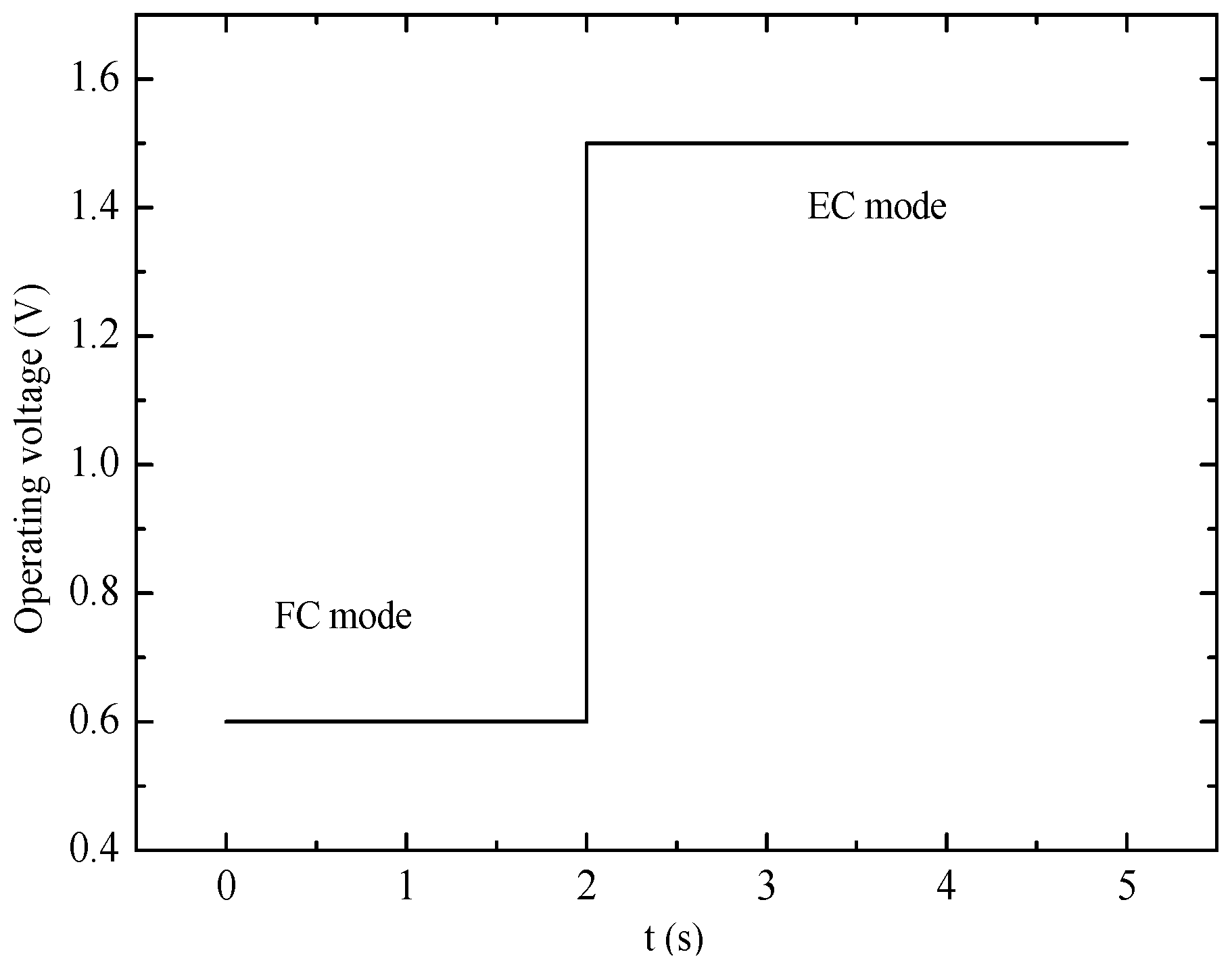
This study deals with the understanding of the dynamic response of an operating PEM-based URFC during the mode switching process. The cell operating mode in FC or EC is controlled by cell voltage, as shown in Figure 5. Cell voltage in the FC and EC modes are set as 0.6 V in the first 2 s and 1.5 V during the subsequent 3 s. In the course of the switching process, the key transient responses of the current density, mass transfer, and heat transmission would occur at approximately 2 s, and the results will be shown and discussed in this section.

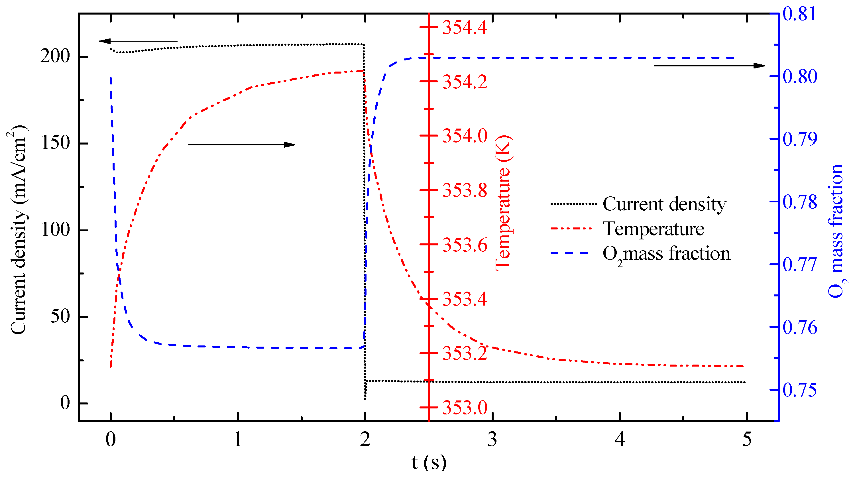
Figure 6 displays the transient responses of current density, O₂ mass fraction and temperature at the central point of the OCL. At the beginning of the FC mode, the O₂ mass fraction declines sharply, whereas the current density and temperature increase gradually because of the consumption of O₂ and the generation of heat. The O₂ mass fraction and current density reach a steady state at approximately 1 s. At 2 s the temperature continues to increase. The current density decreases to 2.77 mA·cm⁻² at 2 s because of mode switching. Then, the current density rapidly increases to approximately 15 mA·cm⁻² corresponding to the EC mode. At the same time, O₂ mass fraction and temperature at that point change dramatically. These changes can be explained as follows: The accumulated water, which is produced in the FC mode, is the reactant in the EC mode. The concentration of H₂O reduces rapidly at the beginning of the EC mode, which leads to a slight decrease in the current density. The O₂ mass fraction increases sharply because of the consumption of H₂O and the production of O₂ when the mode is switched from FC mode to EC mode. Temperature decreases rapidly at 2 s mainly because the exothermic reaction in the FC mode converts into the endothermic reaction in the EC mode. During the subsequent 3 s, the temperature gradient diminishes gradually. Temperature does not reach a steady state during the process. Current density, O₂ mass fraction and temperature in the OCL suddenly change under operation mode switching. The response time of temperature is longer than that of current density and O₂ mass fraction.

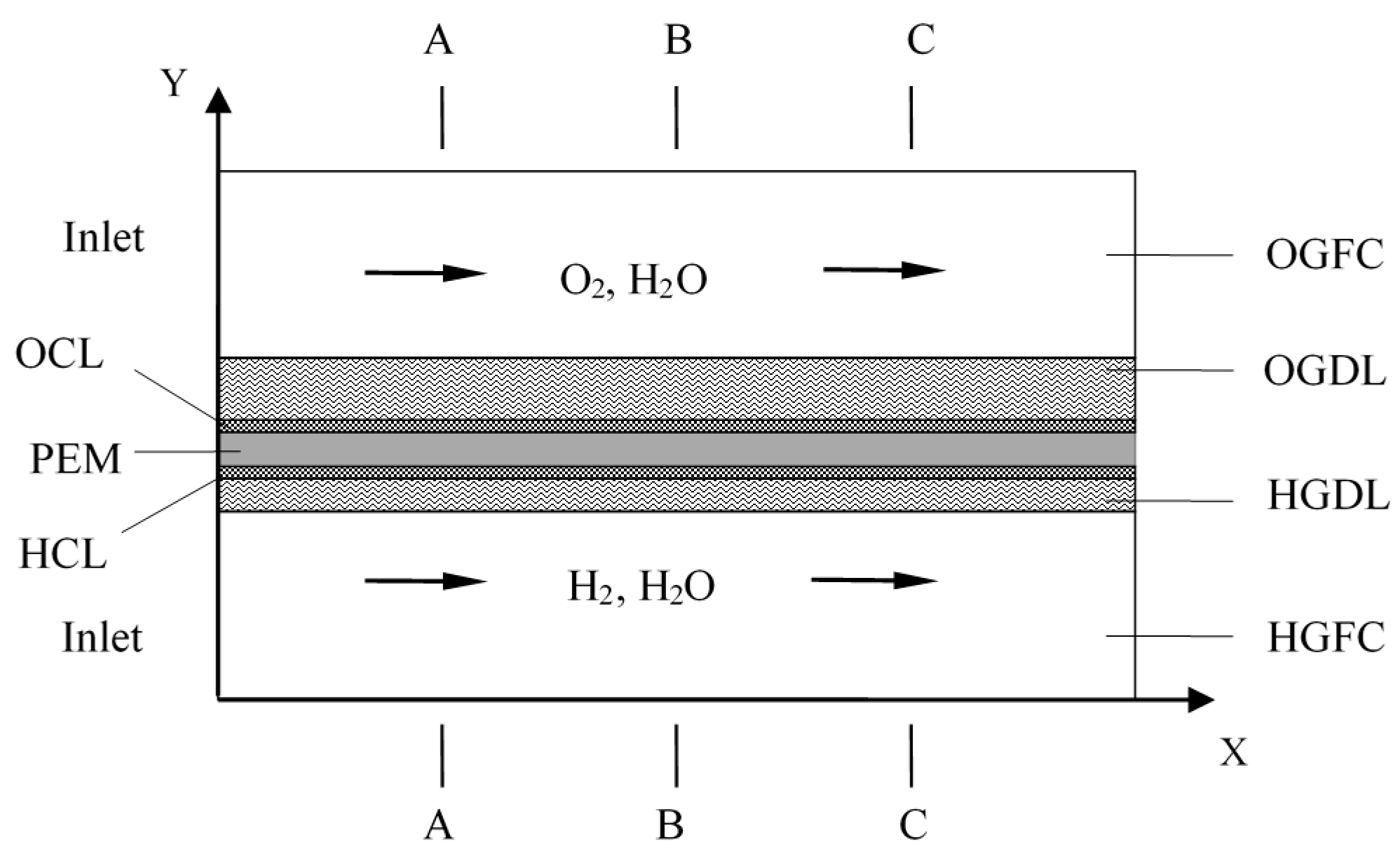
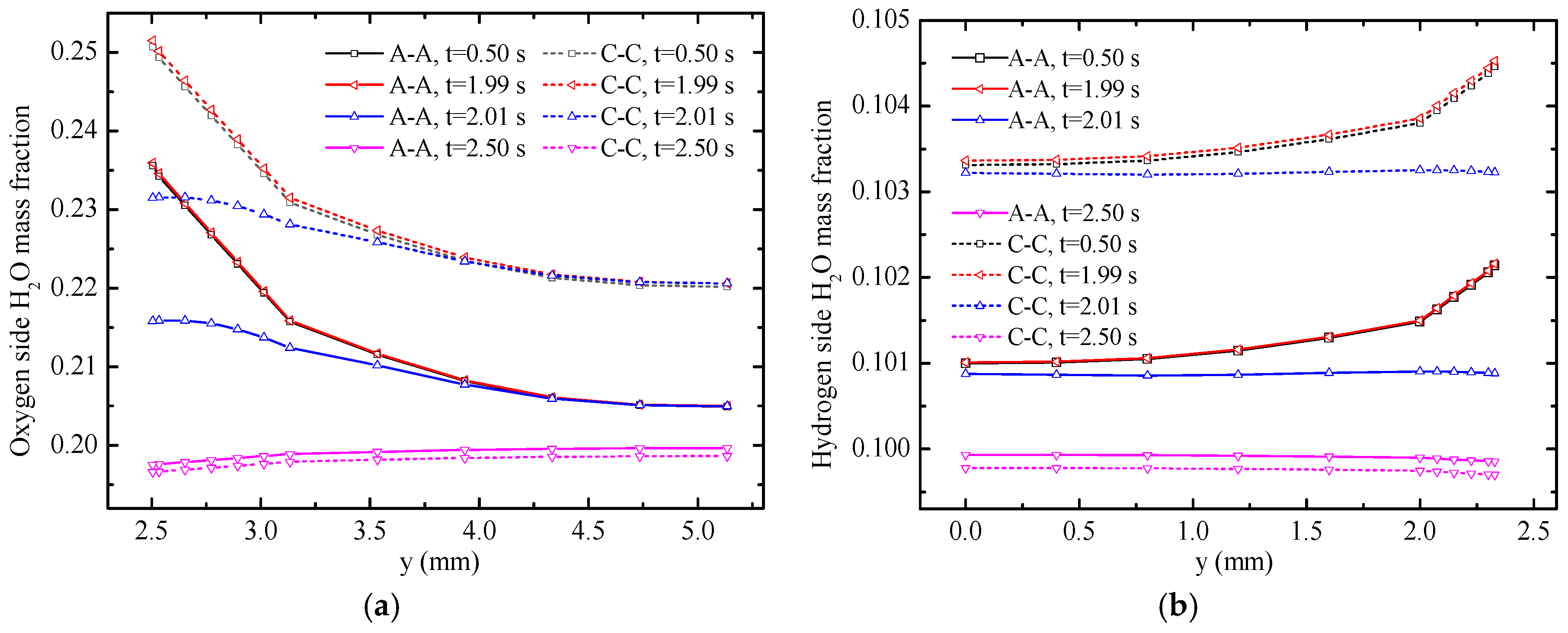
The water mass fractions along y-axis with varying times are displayed in Figure 7. The solid lines represent the temperature distribution along A-A line and the dotted lines represent the temperature distribution along the C-C line. Under the FC mode, the water mass fraction along the C-C line is evidently higher than that along the A-A line. The main reasons are the consumption of reactants and generation of H₂O in oxygen side. Therefore, the H₂O mass fraction increases gradually along the gas flow direction. Moreover, the consumption and the generation of gases occur in the CLs. H₂O mass fraction increases gradually from gas flow channels to CLs because of gas diffusion. However, the distribution of H₂O mass fraction under the EC mode is different from that under the FC mode because of the opposite electrochemical reactions. The mass fraction gradient in the hydrogen side is smaller compared with that in the oxygen side because of the generation of water and the small molecular weight of hydrogen. The water mass fraction at 0.5 and 1.99 s did not change at the A-A line. Meanwhile, at the C-C line, the water mass fraction at 1.99 s is slightly larger than that at 0.05 s, which illustrates that the mass fraction near the inlet of the gas flow channel reaches a steady state faster. The H₂O mass fraction decreases in different degrees within 0.02 s from t = 1.99 s to t = 2.01 s. Along the y-direction from gas flow channel to CLs, the H₂O mass fraction significantly changes. At 2.01 s, the maximum value of H₂O mass fraction appears on the GDLs. The H₂O mass fraction dramatically declines in the CLs because of mode switching from the FC mode to the EC mode at 2.0 s and the opposite electro-chemical reactions of the two modes. Eventually, the H₂O mass fraction declines in the GDLs and gas flow channels under the action of diffusion.

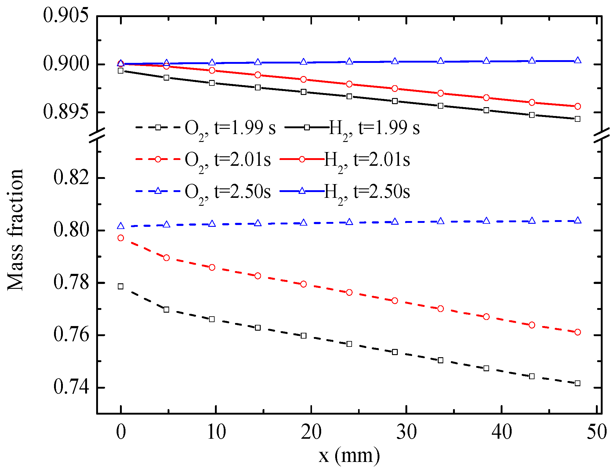
Figure 8 displays the distribution of H₂ and O₂ mass fractions along the central lines of the CLs. The results indicate that both O₂ and H₂ mass fractions are depressed distinctly along the flow direction at 1.99 s. The O₂ and H₂ mass fractions increase when the mode is switched to the EC mode. Eventually, the O₂ and H₂ mass fractions increase along the flow direction under a more stable EC mode at 2.5 s, and the magnitudes of O₂ and H₂ mass fractions are greater than those at the inlets of gas flow channels because of the production of O₂ and H₂ in the CLs. As with the H₂O mass fraction, the gradient of the O₂ mass fraction is significantly larger than that of the H₂ mass fraction.

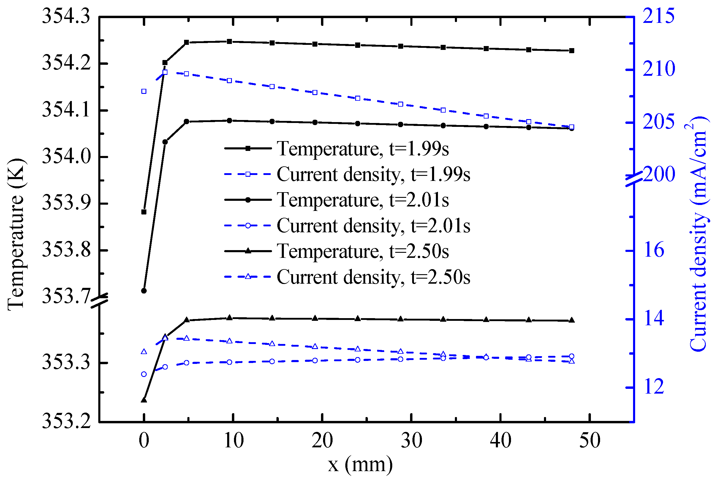
Figure 9 shows the distribution of temperature and current density along the central line of the OCL. At the end of the FC mode (1.99 s), the general trends of temperature and current density decline gradually along the x-axis. The distribution of current density probably results from the concentrations of the reactants. As shown in Figure 8, the O₂ mass fraction declines along the x-axis. The temperature is determined by the heat source and heat flow. For the homogenous and isotropic CL, a relatively high temperature is observed where the heat source is large. The heat source in the OCL consists of heat attributed to activation polarizations, Joule heat, and reaction heat, all of which are positively correlated with current density. Therefore temperature is depressed along the x-axis. Temperature and current density show remarkable reduction during 0.02 s from 1.99 s to 2.01 s. The causes of temperature reduction are varied. The main reasons are the endothermic electrochemical reaction heat source and low current density under the EC mode. However, the current density distribution increases slightly along the x-axis at 2.01 s and decreases at 2.5 s. The main reason for these trends is the change of H₂O concentration, which has an opposite distribution trend compared with O₂. From the O₂ mass fraction shown in Figure 8, the concentration of H₂O, which is reactant for the reaction of the EC mode, has a distribution trend similar to current density along the x-axis. The temperature at the OCL exhibits an evident decrease in the process of operation mode switching. The temperature difference along the x-axis is less than 0.1 K, except at the left end. The current density, temperature, and mass fraction of the reactant influence each other to some extent.

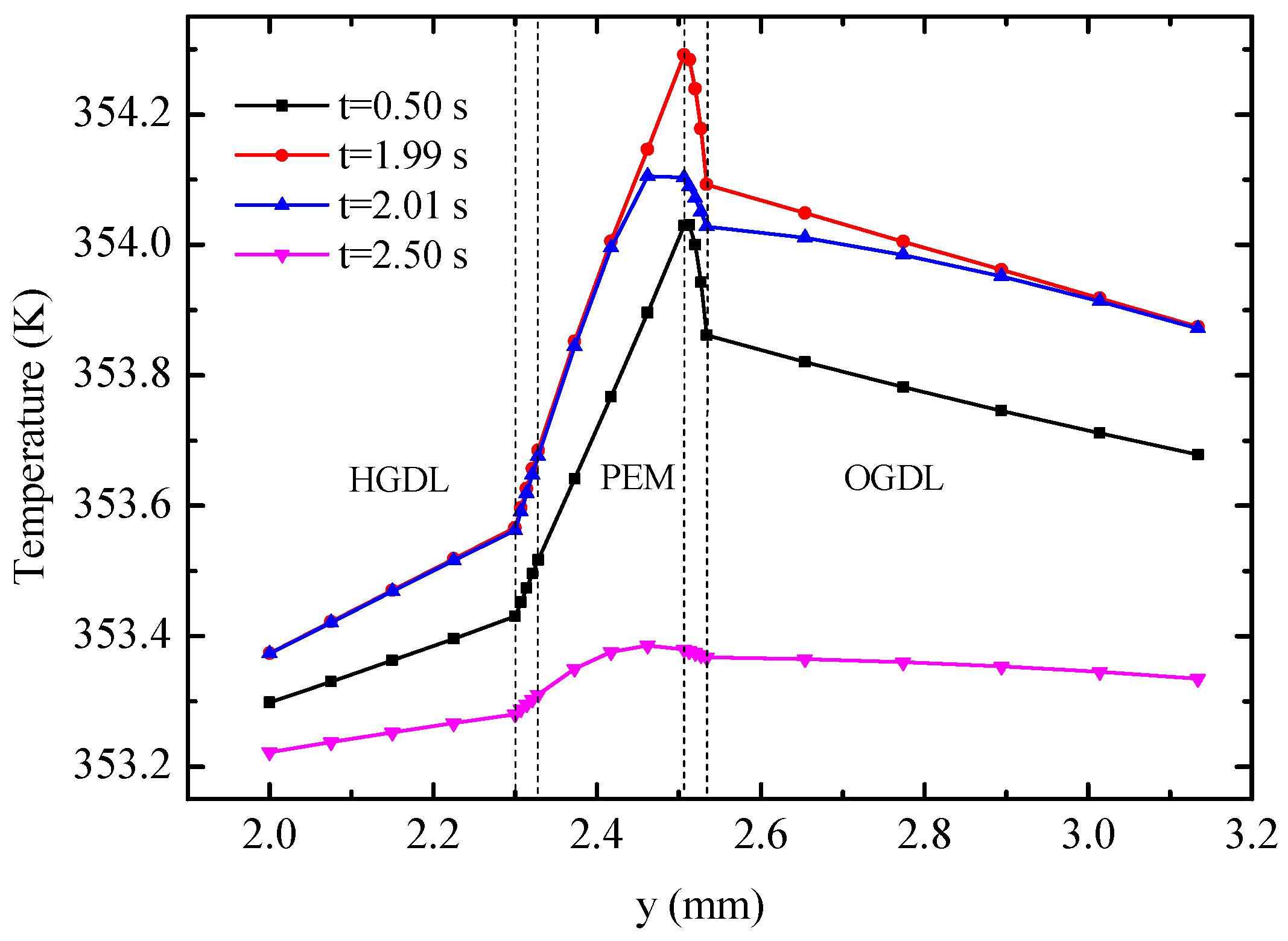
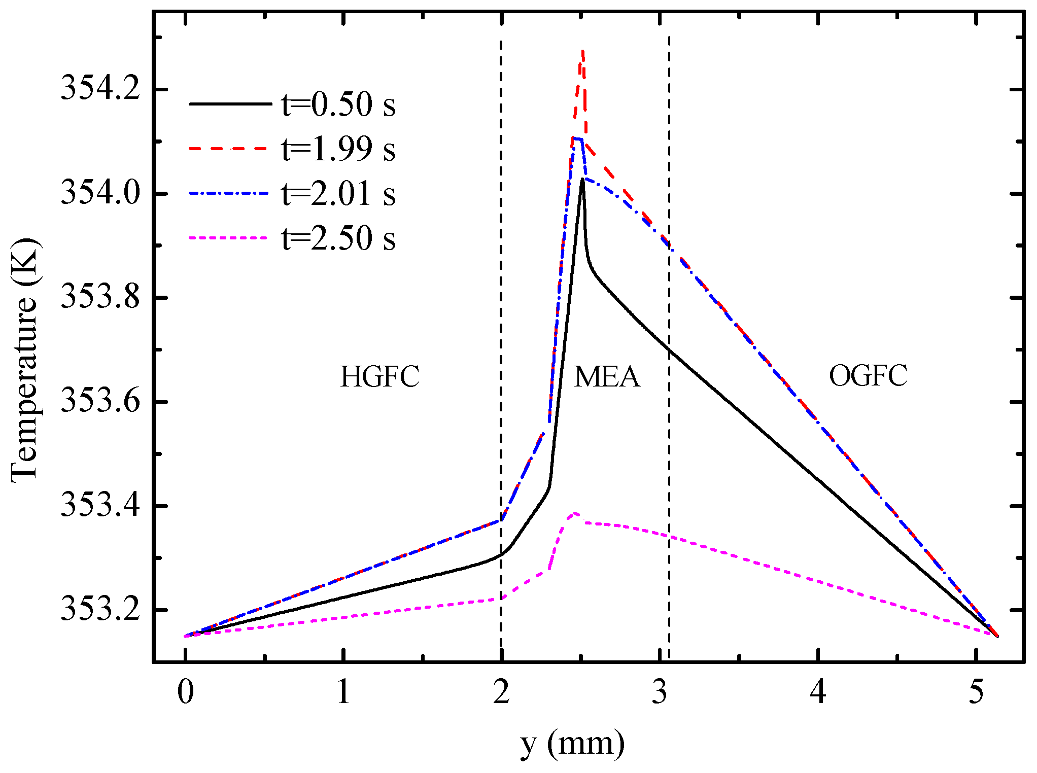
Figure 10 displays the temperature profiles of the cell along line B-B at different times. Figure 11 shows the detailed temperature distribution of the MEA. As shown in Figure 10, temperature in the hydrogen side is lower than that in the oxygen side, which can be explained by the following three factors: (1) The heat source in OCL accounts for more than 90% of all heat sources according to

Table 3. Heat sources of electrodes and percentages in different times.

Time (s)		0.5	1.99	2.01	2.5	4
OGDL	Heat source(W·m−1)	0.4715	0.4798	0.0025	0.0023	0.0022
	Percentage	0.27%	0.27%	10.55%	10.09%	9.95%
HGDL	Heat source(W·m−1)	0.2358	0.2399	0.0013	0.0012	0.0011
	Percentage	0.14%	0.14%	5.49%	5.26%	4.98%
PEM	Heat source(W·m−1)	11.7206	11.9004	0.0623	0.0585	0.0558
	Percentage	6.72%	6.76%	262.87%	256.58%	252.49%
OCL	Heat source(W·m−1)	158.2474	159.5226	−0.0627	−0.0581	−0.0550
	Percentage	90.7%	90.64%	−264.56%	−254.82%	−248.87%
HCL	Heat source(W·m−1)	3.7937	3.8588	0.0203	0.0189	0.0180
	Percentage	2.17%	2.19%	85.65%	82.89%	81.45%
Total heat source		100%	100%	100%	100%	100%

; (2) the thickness of OGDL is double that of HGDL, which causes double Joule heat; and (3) the heat conductivity of oxygen is smaller than that of hydrogen. In spite of the endothermic reaction in the EC mode, the temperature in the hydrogen side is lower than that in the oxygen side during the limited time of this mode because of the heat attributed to activation polarizations, Joule heat, and heat accumulation in the FC mode. The maximum value of temperature appears at the OCL and increases gradually under the FC mode. During the 0.02 s from 1.99 s to 2.01 s, the temperature of the oxygen electrode decreases sharply, but the temperature of other areas almost remains constant. The main reason for these results is that the OCL is the place where heat source exhibits the most significant changes. Furthermore, the low conductivity of the membrane hinders heat transfer to the hydrogen side. After the EC process lasting 0.5 s, at 2.5 s, the maximum of temperature appears at the membrane on account of the largest value of heat source according to Table 3. The temperature of the entire B-B line decreases to different degrees.

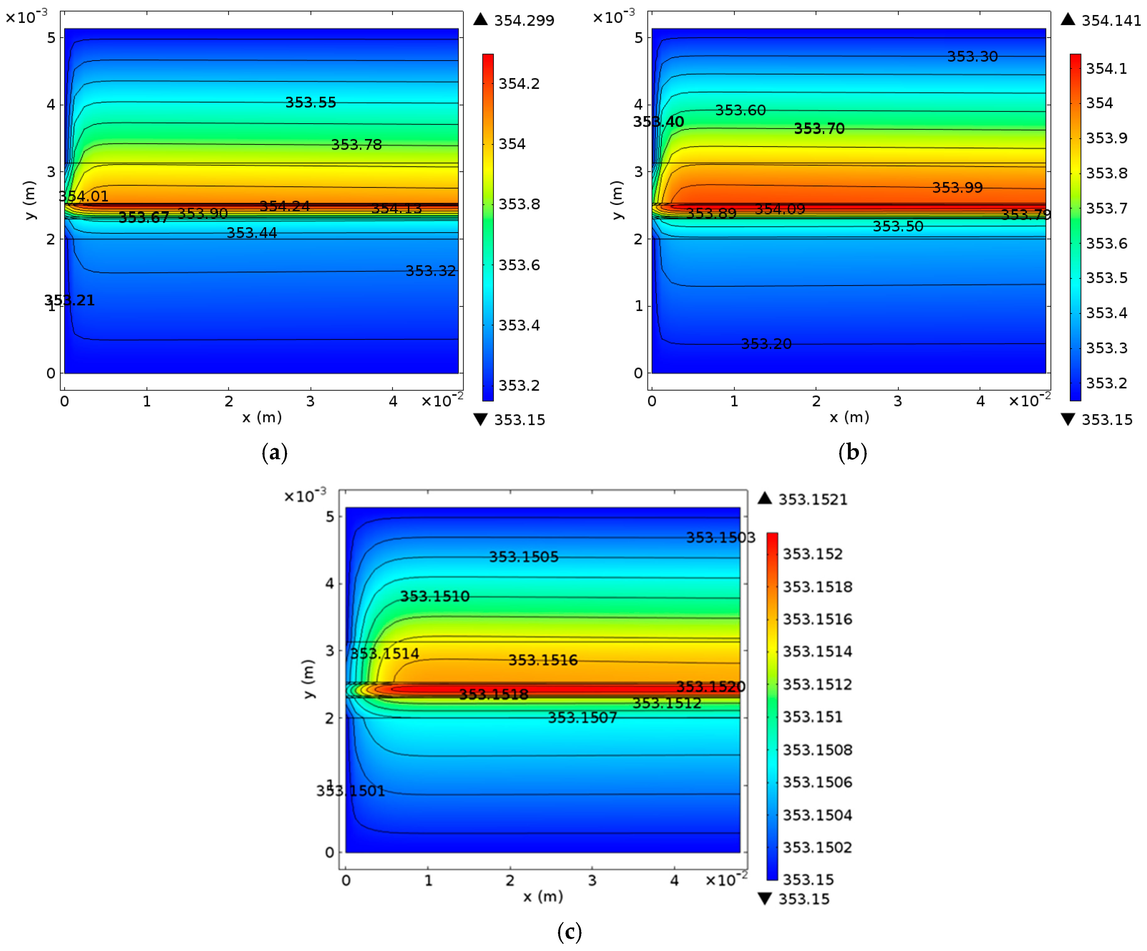
Similar phenomena and conclusion can be observed and drawn from Figure 12, which shows transient variations of the entire cell temperature. Under the FC mode, the temperature in the OCL is significantly higher than that in other areas. The temperature difference decreases when the mode is switched to the EC mode. The maximum temperature difference is less than 1.5 K. By the time the EC reaches a more stable state, the cell temperature is slightly higher than the operating temperature, and the highest temperature appears at the membrane. In addition, the cell temperature distribution trends along the x-axis are similar at different times. The temperature gradient near the inlet is relatively large and exhibit a small temperature change along the x-axis behind x = 0.05 m.

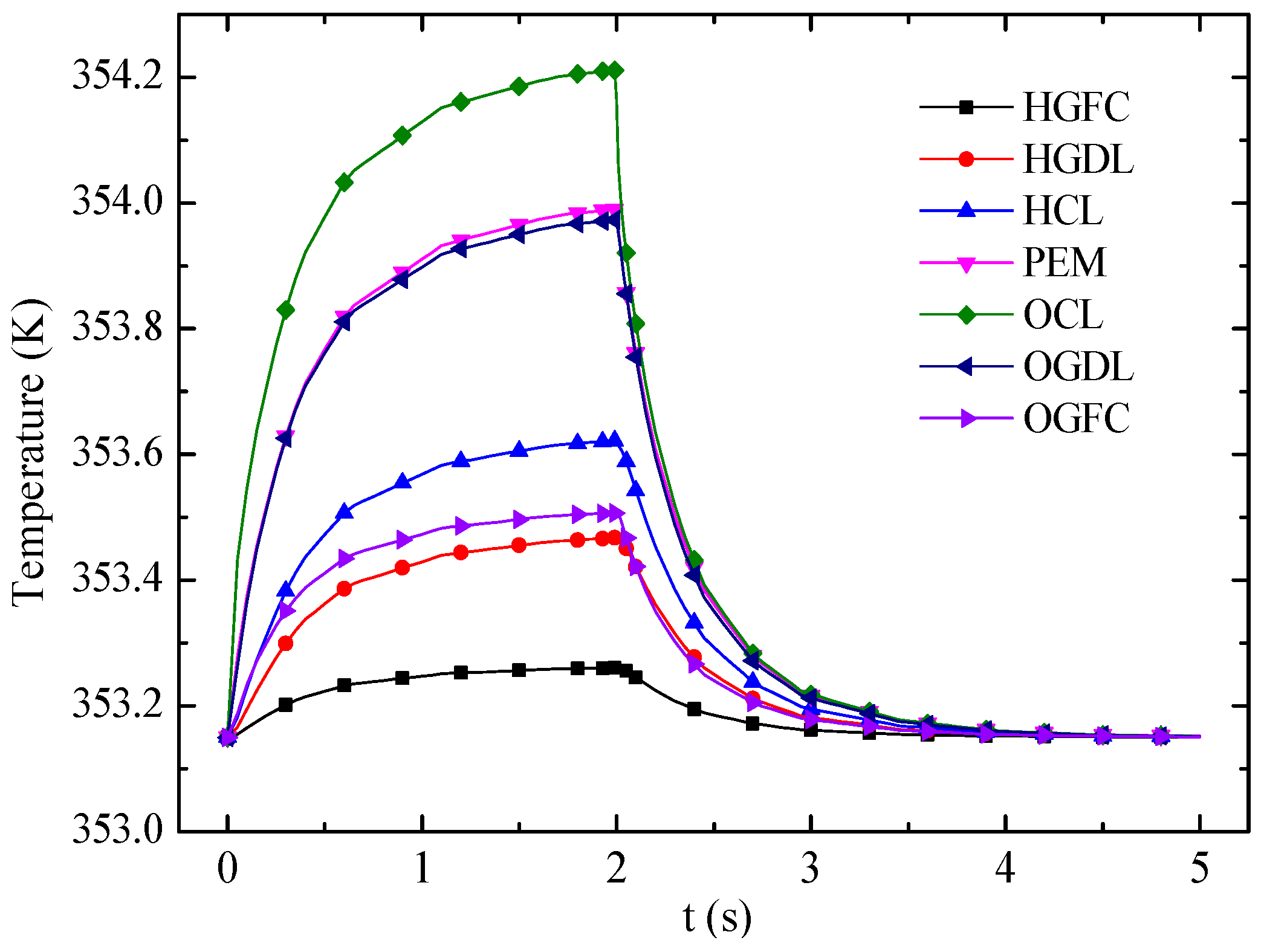
Figure 13 shows the transient responses of average temperature in different layers. The OCL, which generates the most heat under the FC mode but absorbs heat under the EC mode, has the strongest temperature variation. In the FC mode, the temperature of each layer increases with time because of heat accumulation. Then the temperature variation becomes small and decreases rapidly when the cell mode is switched from FC mode to EC mode at 2 s. The temperatures of the CLs are close to that of the membrane under the EC mode. Eventually, the temperature difference of entire cell is small because of the endothermic reaction and the small current density in the EC mode.

Table 3 lists the heat sources and its percentages in each layer before and after mode switching. Under the FC mode, heat attributed to activation polarizations and reaction heat are the main sources of cell total heat production, and Joule heat contributes less than 10% of all heat. When the mode is switched to EC, cell total heat production comes mainly from Joule heat in the membrane, and the value of the heat source in the OCL is negative because of the endothermic reaction. However, the cell is still exothermic, although the total heat is small under the EC mode.

5. Conclusions

In this study, a transient, non-isothermal, and multi-physics model for a PEM URFC is developed, in which the electrochemical reaction is also coupled. The model is validated, and results are consistent with the previously published experimental results. Numerical simulations are conducted to investigate the transient responses of heat and mass transfer as well as current density in a URFC when the operating mode is switched from FC mode to EC mode. The results, which considered the temperature, gas mass fractions, current density, and heat source, are shown and discussed. The following conclusions can be obtained:

(1)

Mode switching has a significant effect on heat and mass transfer in PEM URFCs. The dynamic responses of temperature, mass fraction and current density are different. The response time of temperature is longer than that of current density and gas mass fractions.

(2)

The mass fraction of H₂O along the direction from gas flow channel to CL and the gas flow direction changes into a decreasing trend in the EC mode from an increasing trend in the FC mode. H₂ and O₂ reveal an opposite mass fraction distribution trend compared with H₂O. The gradient of gas mass fractions in the oxygen side is larger than that in the hydrogen side along x- and y-axes.

(3)

Cell temperature in the hydrogen side is lower than that in the oxygen side under the FC and EC modes. The temperature difference of the entire cell is less than 1.5 K. The highest temperature appears at the OCL under the FC mode. Under the EC mode, the highest temperature initially exists at the OCL and then at the membrane.

(4)

The OCL, which generates the most heat under the FC mode but absorbs heat under the EC mode, has the strongest temperature variation when the cell operates from the FC mode to the EC mode.

(5)

The cell is exothermic under the FC and EC modes. The heat attributed to activation polarizations and reaction heat in the OCL occupies a dominant part of heat production under the FC mode. Meanwhile, in the EC mode, Joule heat in the membrane mainly contributes to heat production.

References

1. Gabbasa, M.; Sopian, K.; Fudholi, A. A review of unitized regenerative fuel cell stack: Material, design and research achievements. Int. J. Hydrog. Energy 2014, 39, 17765–17778. [Google Scholar] [CrossRef]
2. Grigorievs, A.; Millet, P.; Porembsky, V.I. Development and preliminary testing of a unitized regenerative fuel cell based on PEM technology. Int. J. Hydrog. Energy 2011, 36, 4164–4168. [Google Scholar] [CrossRef]
3. Mitlitsky, F.; Myers, B.; Weisberg, A.H. Reversible PEM fuel cell devices. Fuel Cells Bull. 1999, 11, 6–11. [Google Scholar] [CrossRef]
4. Doddathimmaiah, A.K.; Andrews, J. The use of PEM unitised regenerative fuel cells in solar-hydrogen systems for remote area power supply. In Proceedings of the World Hydrogen Energy Conference, Lyon, France, 13–16 June 2006.
5. Applyby, A.P. Regenerative fuel cells for space applications. J. Power Sources 1988, 22, 377–385. [Google Scholar] [CrossRef]
6. Millet, P.; Ngameni, R.; Grigoriev, S.A. Scientific and engineering issues related to PEM technology: Water electrolysers, fuel cells and unitized regenerative systems. Int. J. Hydrog. Energy 2011, 36, 4156–4163. [Google Scholar] [CrossRef]
7. Guo, S.M. Design and testing of a unitized regenerative fuel cell. J. Fuel Cell Sci. Technol. 2009, 6. [Google Scholar] [CrossRef]
8. Alotto, P.; Guarnieri, M. Multi-physics model for regenerative PEM fuel cell energy storage. In Proceedings of the 2013 IEEE International Conference on Industrial Technology (ICIT), Cape Town, South Africa, 25–28 February 2013; pp. 746–751.
9. Guarnieri, M.; Alotto, P.; Moro, F. Modeling the performance of hydrogen-oxygen unitized regenerative proton exchange membrane fuel cells for energy storage. J. Power Sources 2015, 297, 23–32. [Google Scholar] [CrossRef]
10. Grigoriev, S.A.; Millet, P.; Dzhus, K.A. Design and characterization of bi-functional electrocatalytic layers for application in PEM unitized regenerative fuel cells. Int. J. Hydrog. Energy 2010, 35, 5070–5076. [Google Scholar] [CrossRef]
11. Roca-Ayats, M.; Garcia, G.; Galante, J.L. Electrocatalytic stability of Ti based-supported Pt3Ir nanoparticles for unitized regenerative fuel cells. Int. J. Hydrog. Energy 2014, 39, 5477–5484. [Google Scholar] [CrossRef]
12. Cruz, J.C.; Baglio, V.; Siracusano, S. Nanosized Pt/IrO2 electrocatalyst prepared by modified polyol method for application as dual function oxygen electrode in unitized regenerative fuel cells. Int. J. Hydrog. Energy 2012, 38, 5508–5517. [Google Scholar] [CrossRef]
13. Ioroi, T.; Yasuda, K.; Siroma, Z.; Fujiwara, N.; Miyazaki, Y. Thin film electrocatalyst layer for unitized regenerative polymer electrolyte fuel cells. J. Power Sources 2002, 112, 583–587. [Google Scholar] [CrossRef]
14. Jung, H.Y.; Huang, S.Y.; Ganesan, P. Performance of gold-coated titanium bipolar plates in unitized regenerative fuel cell operation. J. Power Sources 2009, 194, 972–975. [Google Scholar] [CrossRef]
15. Zhang, H.B.; Hou, M.; Lin, G.Q. Performance of Tie-Ag-deposited titanium bipolar plates in simulated unitized regenerative fuel cell (URFC) environment. Int. J. Hydrog. Energy 2011, 36, 5695–5701. [Google Scholar] [CrossRef]
16. Huang, S.Y.; Ganesan, P.; Jung, H.Y. Development of supported bi-functional oxygen electro-catalysts and corrosion-resistant gas diffusion layer for unitized regenerative fuel cell applications. J. Power Sources 2012, 198, 23–29. [Google Scholar] [CrossRef]
17. Huang, S.Y.; Ganesan, P.; Jung, H.Y. Comparison of corrosion behaviors between SS304 and Ti substrate coated with (Ti,Zr)N thin films as Metal bipolar plate for unitized regenerative fuel cell. J. Power Sources 2013, 544, 162–169. [Google Scholar]
18. Chen, G.B.; Zhang, H.M.; Ma, H.P. Effect of fabrication methods of bifunctional catalyst layers on unitized regenerative fuel cell performance. Electrochim. Acta 2009, 54, 5454–5462. [Google Scholar] [CrossRef]
19. Ito, H.; Miyazaki, N.; Ishida, M.; Nakano, A. Efficiency of unitized reversible fuel cell systems. Int. J. Hydrog. Energy 2016, 41, 5803–5815. [Google Scholar] [CrossRef]
20. Li, S.L.; Sui, S.H.; Shi, W.C.H. Investigation of MEA and flow-field in unitized regenerative fuel cell. Chin. J. Power Sources 2011, 35, 1235–1239. [Google Scholar]
21. Zhang, X.R.; Wang, T.; Zhang, W. Performance of unitized regenerative fuel cell. Chem. Ind. Eng. Prog. 2011, 30, 734–738. [Google Scholar]
22. Doddathimmaiah, A.K.; Andrews, J. Theory, modelling and performance measurement of unitized regenerative fuel cells. Int. J. Hydrog. Energy 2009, 34, 8157–8170. [Google Scholar] [CrossRef]
23. Wang, L.L.; Guo, H.; Ye, F. Two-dimensional simulation of mass transfer in unitized regenerative fuel cells under operation mode switching. Energies 2016, 9, 47. [Google Scholar] [CrossRef]
24. Jin, X.F.; Xue, X.J. Mathematical modeling analysis of regenerative solid oxide fuel cells in switching mode conditions. J. Power Sources 2010, 195, 6652–6658. [Google Scholar] [CrossRef]
25. Liu, J.X.; Guo, H.; Ye, F.; Qiu, D.C.; Ma, C.F. Interfacial phenomena and heat transfer in proton exchange membrane fuel cells. Interfacial Phenom. Heat Transf. 2015, 3, 259–301. [Google Scholar] [CrossRef]
26. Acosta, M. Modeling non-isothermal two-phase multi -component flow in the cathode of PEM fuel cells. J. Power Sources 2006, 18, 21–28. [Google Scholar]
27. Ju, H.; Hua, M.; Wang, C.Y. A single-phase, non-isothermal model for PEM fuel cells. Int. J. Heat Mass Transf. 2005, 48, 1303–1315. [Google Scholar] [CrossRef]
28. Wen, X.F. Thermal Modeling and Software Development of Proton Exchange Membrane Fuel Cell. Master’s Thesis, Wuhan University of Technology, Wuhan, China, March 2005. [Google Scholar]
29. Adzakpa, K.P.; Ramousse, J.; Dub, Y. Transient air cooling thermal modeling of a PEM fuel cell. J. Power Sources 2008, 179, 164–176. [Google Scholar] [CrossRef]
30. Khakbaz, M.; Babol, I.; Kermani, M.J. A two-dimensional, transient, compressible isothermal and two-phase model for the air-side electrode of PEM fuel cells. Electrochim. Acta 2008, 53, 7644–7654. [Google Scholar] [CrossRef]
31. Dadda, B.; Abboudi, S.; Ghezal, A. Transient two-dimensional model of heat and mass transfer in a PEM fuel cell membrane. Int. J. Hydrog. Energy 2013, 38, 7092–7101. [Google Scholar] [CrossRef]
32. Meng, H. Numerical investigation of transient responses of a PEM fuel cell using a two-phase non-isothermal mixed-domain model. J. Power Sources 2007, 171, 738–746. [Google Scholar] [CrossRef]
33. Chandesris, M.; Medeau, V.; Guillet, N. Membrane degradation in PEM water electrolyzer: Numerical modeling and experimental evidence of the influence of temperature and current density. Int. J. Hydrog. Energy 2015, 40, 1353–1366. [Google Scholar] [CrossRef]
34. Marangio, F.; Santarelli, M.; Call, M. Theoretical model and experimental analysis of a high pressure PEM water electrolyser for hydrogen production. Int. J. Hydrog. Energy 2009, 34, 1143–1158. [Google Scholar] [CrossRef]
35. Hamour, M.; Garnier, J.P.; Grandidier, J.C. Thermal-conductivity characterization of gas diffusion layer in proton exchange membrane fuel cells and electrolyzers under mechanical loading. Int. J. Thermophys. 2011, 32, 1025–1037. [Google Scholar] [CrossRef]
36. Raj, A.; Shamim, T. Investigation of the effect of multidimensionality in PEM fuel cells. Energy Convers. Manag. 2014, 86, 443–452. [Google Scholar] [CrossRef]
37. Ju, H.; Wang, C.Y. Experimental validation of a PEM fuel cell model by current distribution data. J. Electrochem. Soc. 2004, 151, A1954–A1960. [Google Scholar] [CrossRef]
38. Hu, G.L.; Fan, J.R. A three-dimensional, multicomponent, two-phase model for a proton exchange membrane fuel cell with straight channels. Energy Fuels 2006, 20, 738–747. [Google Scholar] [CrossRef]
39. Cao, T.F.; Lin, H.; Chen, L. Numerical investigation of the coupled water and thermal management in PEM fuel cell. Appl. Energy 2013, 112, 1115–1125. [Google Scholar] [CrossRef]
40. Ubong, E.U.; Shi, Z.; Wang, X. Three-dimensional modeling and experimental study of a high temperature PBI-based PEM fuel cell. J. Electrochem. Soc. 2009, 156, B1276–B1282. [Google Scholar] [CrossRef]
41. Doubek, G.; Robalinho, E.; Cunha, E.F. Application of CFD techniques in the modeling and simulation of PBI PEMFC. Fuel Cells 2011, 11, 764–774. [Google Scholar] [CrossRef]
42. Sehribani, U. Mathematical and Computational Modeling of Polymer Exchange Membrane Fuel Cells. Master’s Thesis, University of Nevada, Reno, NV, USA, August 2012. [Google Scholar]
43. Cussler, E.L. Diffusion-Mass Transfer in Fluid Systems; Cambridge University Press: London, UK, 1969. [Google Scholar]
44. Sun, P.T. A Dirichlet/Robin iteration-by-subdomain method for an anisotropic, non-isothermal two-phase transport model of PEM fuel cell with micro-porous layer. J. Comput. Appl. Math. 2014, 270, 241–256. [Google Scholar] [CrossRef]
45. Xing, L.; Liu, X.T.; Alaje, T. A two-phase flow and non-isothermal agglomerate model for a proton exchange membrane (PEM) fuel. Energy 2014, 73, 618–634. [Google Scholar] [CrossRef]
46. Leyens, C.; Peters, M. Titanium and Titanium Alloys; John Wiley & Sons Inc.: Hoboken, NJ, USA, 2003. [Google Scholar]
47. Banerjee, R.; Bazylak, A. Modeling heat transfer through phase-differentiated nano-scale constructions of polymer electrolyte membrane fuel cell micro-porous layers. Int. J. Heat Mass Transf. 2016, 92, 131–138. [Google Scholar] [CrossRef]
48. Wu, H.; Peter, B.; Li, X.G. Non-isothermal transient modeling of water transport in PEM fuel cells. J. Power Sources 2007, 165, 232–243. [Google Scholar] [CrossRef]
49. Shan, Y.Y.; Choe, S.Y.; Choi, S.H. Unsteady 2D PEM fuel cell modeling for a stack emphasizing thermal effects. J. Power Sources 2007, 165, 196–209. [Google Scholar] [CrossRef]
Figure 1. Computational domain of the 2D proton exchange membrane (PEM) unitized regenerative fuel cell (URFC). OGDL: oxygen-side gas diffuse layer; HGDL: hydrogen-side gas diffuse layer; OGFC: oxygen-side gas flow channels; and HGFC: hydrogen-side gas flow channels.
Energies 09 01015 g001
Figure 2. Schematic of the rib and the gas flow channel.
Energies 09 01015 g002
Figure 3. Element independence test for the present model: (a) temperature distribution of the central line of the membrane with an operating voltage of 0.6 V; and (b) temperature distribution of the central line of the OCL with an operating voltage of 1.8 V.
Energies 09 01015 g003
Figure 4. Comparison of the computed URFC performance with the experimental results [2,3]: (a) operating temperature T = 353.15 K; and (b) operating temperature T = 363.15 K.
Energies 09 01015 g004
Figure 5. Operating voltage setting under mode switching.
Energies 09 01015 g005
Figure 6. Time-dependent evolution of relevant parameters in the central point of the OCL.
Energies 09 01015 g006
Figure 7. Water mass fraction distribution along lines A-A and C-C: (a) oxygen side; and (b) hydrogen side.
Energies 09 01015 g007
Figure 8. H2 and O2 mass fraction distribution at different time.
Energies 09 01015 g008
Figure 9. The distribution of temperature and current density.
Energies 09 01015 g009
Figure 10. Temperature profiles along the B-B plane of the entire cell. MEA: membrane electrode assembly.
Energies 09 01015 g010
Figure 11. Temperature profiles along the B-B plane of the MEA.
Energies 09 01015 g011
Figure 12. Transient variations of temperature inside the URFC: (a) t = 1.99 s; (b) t = 2.01 s; and (c) t = 5.00 s.
Energies 09 01015 g012
Figure 13. Transient responses of average temperature in different layers.
Energies 09 01015 g013