A Comparison of Impedance-Based Fault Location Methods for Power Underground Distribution Systems

Abstract

In the last few decades, the Smart Grid paradigm presence has increased within power systems. These new kinds of networks demand new Operations and Planning approaches, following improvements in the quality of service. In this sense, the role of the Distribution Management System, through its Outage Management System, is essential to guarantee the network reliability. This system is responsible for minimizing the consequences arising from a fault event (or network failure). Obviously, knowing where the fault appears is critical for a good reaction of this system. Therefore, several fault location techniques have been proposed. However, most of them provide individual results, associated with specific testbeds, which make the comparison between them difficult. Due to this, a review of fault location methods has been done in this paper, analyzing them for their use on underground distribution lines. Specifically, this study is focused on an impedance-based method because their requirements are in line with the typical instrumentation deployed in distribution networks. This work is completed with an exhaustive analysis of these methods over a PSCAD^TM X4 implementation of the standard IEEE Node Test Feeder, which truly allows us to consistently compare the results of these location methods and to determine the advantages and drawbacks of each of them.

1. Introduction

The energy needs and quality requirements of our society have been increasing in the last few decades. These improvements follow the lead of the new Smart Grid (SG) tendencies [1,2,3,4]. Moreover, the improvement of the quality of service is one of their main priorities [5,6]. Thus, an essential characteristic of a SG network is its strong Distributed Generation (DG) [7] and Distributed Energy Storage (DES) [8] presence, which together with Demand-Side Management (DSM) [9,10] systems make up microgrids [11] and provide improvements in the network reliability [12]. However, this presence shifts the traditional philosophy of Transmission and Distribution (T&D) systems, adding bidirectional energy flows along them. Unfortunately, as will be seen below, these changes in the flow directions are a significant constraint on network fault analysis, requiring complex systems to guarantee a proper operation in these environments.

In this sense, this SG network seeks the Self-Healing [13] concept where Fault Detection, Isolation and Restoration (FDIR) [14] philosophy is applied by the Outage Management System (OMS) to improve the network operation, automatically solving or mitigating the fault consequences. Specifically, a self-healing grid is a system which detects and isolates faults and reconfigures the distribution network, reducing the impact of an electrical fault and improving the resiliency of the network. Self-healing is not a new concept. For decades, electric utilities have been implementing automatic reclosers to restore the power supply without human intervention. However, current electric distribution utilities are big and complex systems and commonly operate in a high load factor. In this scenario, self-healing systems need to be more intelligent, acting in real-time to locate the fault and to efficiently reconfigure the topology on SG networks.

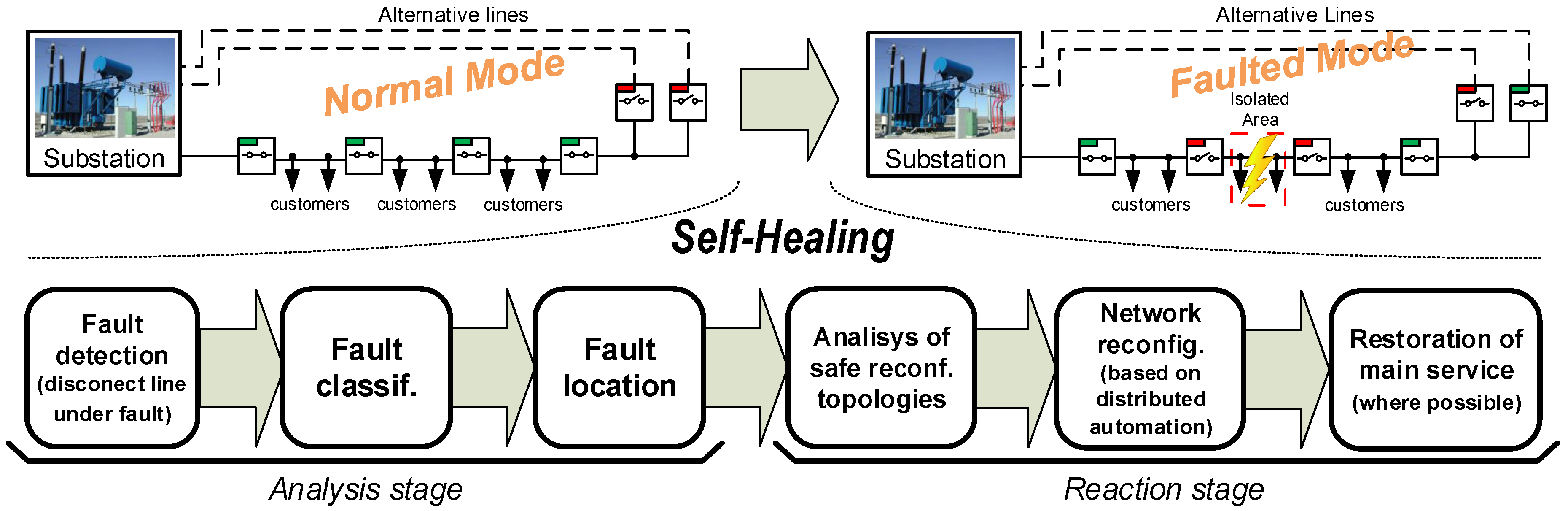
Thus, as can be seen in Figure 1, when a fault happens in a self-healing power network, it is easy to distinguish two main stages.

Firstly, the analysis stage is executed. In this stage, the OMS protects the feeder and characterizes the fault (type, position, etc.). Immediately after, in the reaction stage, the OMS reconfigures the affected network, according to the results obtained from the analysis stage, and restores the supply to as many customers as possible. On the one hand, time spent on this second stage (associated with isolation and restoration procedures) directly depends on the automation level of each network. An example of this fact is presented in [15], where the need of a holistic Distribution Automation (DA) integration is discussed. Additionally, a novel approach that integrates protection, control, and monitoring based on DA is also proposed. On the other hand, the analysis stage requires different studies, and it is typically divided into four steps: detection, classification, and location analyses.

Obviously, the first step (fault detection) should be fast. It is typically associated with Digital Protective Relays (DPRs), which measure voltage and current and quickly disconnect the line under fault conditions. They are typically based on sequential components [16] and impedance [17] analysis. Additionally, other methods use spectral analyses such as Fast Fourier Transform (FFT) [18] or Discrete Wavelet Transform (DWT) [19].

The purpose of the second step is to extract features and to classify faults using the information captured by DPRs or Digital Fault Recorders (DFRs). Traditionally, these techniques apply direct analysis over symmetrical components [20] or use spectral analysis (such as FFT [18] or DWT [21]) to extract the fault features. These studies are commonly supported by computational intelligence, such as Artificial Neural Networks (ANNs) [22], Fuzzy Logic (FL) [23], Decision Trees (DTs) [24] or Support Vector Machines (SVMs) [25].

Finally, the fault location (third step) is responsible for finding the position where the fault occurs. Obviously, a good estimation of this position is essential for the next stages (e.g., isolate the fault). As a proof of its importance, we found the recently reedited IEEE C37.114 standard [26], where the most relevant techniques are summarized. However, as will be seen below, these techniques are quite conditioned by the network topology [27,28] and especially by the presence of DG.

Thus, as was described above, fault location is an essential issue in SG systems. However, this concept has been widely used in transmission networks. Conversely, in distribution networks, they are less common because typically, this network level has complex topologies and limitations in its instrumentation. Fortunately, in the last few years, this tendency is changing. Following the SG philosophy and supported by Information and Communication Technologies (ICT), the fault location analysis is being extended to distribution networks [29]. Besides, the use of underground lines is more common everyday in urban areas, which poses new challenges to apply some location methods.

In this sense, a review of several location methods for distribution networks has been done in this paper. As can be seen below, this work is focused on impedance-based methods because they are more applicable on distribution networks (due to it having less instrumentation requirements). This study compares several location methods highlighting their problems and dependencies, mainly associated with underground scenarios (increasingly common in modern networks, especially in urban environments). Moreover, the main advantage provided in this paper is the use of a standard network as a testbed (unusual in individual studies), allowing us to truly compare coherently amongst these analyzed methods, and providing the ability to compare with other proposals in future work.

Therefore, this paper is divided as follows; Section 2 shows a brief overview of traditional fault location methods. Following this review, Section 3 is focused on the impedance-based fault location methods, analyzing their two main approaches, and describing some relevant examples of them. Section 4 describes the testbed characteristics and poses the simulation set for it. A comparative analysis of the studied methods and its dependency on the parameter variations in the simulated cases is shown in Section 5. Finally, conclusions are shown in Section 6.

2. Fault Location Family Methods Overview

As discussed above, a fast fault location technique is key to improving the OMS. However, theses techniques directly depend on the measurement characteristics. In this sense, they are divided into three families: based on traveling waves; based on high-frequency measurements; and based on phasor measurements.

• Traveling Waves (TW) methods are based on the analysis of propagation time associated with fault effects [30]. This time is measured at one-end (taking advantage of the wave reflections [31]) or multi-end (analyzing the time differences or the delay between them [32]). Unfortunately, this family poses complications under complex topologies (with many reflections). Due to this, it requires the combined use of advanced feature extraction techniques (e.g., DWT combined with Multi-Resolution Analysis, MRA [33]) and classification techniques, the last of them being based on computational intelligence such as Artificial Neural Networks (ANN) [34,35] or Support Vector Machines (SVM) [36] to solve this problem.
• High frequency based methods determine the fault position using high frequency information contained within voltage and current measurements. In this sense, it is possible to distinguish two approaches: time domain methods [37,38,39], or frequency domain methods where MRA [40] is one of their most common tools. Thus, this approach traditionally is also supported by any of the classification techniques, such as ANN [41], FL [42], a combination of both, Adaptive-Network-based Fuzzy Inference System (ANFIS) [43], etc.
• Phasor based methods determine the fault position based on the relationship between main harmonic (or phasor) of voltages and currents. It is the most commonly used family in distribution networks because it has the least requirements for their measurements. The most traditional implementations are based on one-end measurements [44,45,46,47,48,49,50,51] and are commonly known as apparent impedance methods. These methods only need a voltage and current measurement (typically registered at line header). Conversely, two-end (or multi-end) methods [52,53,54,55,56,57,58] use measurements at several nodes, analyzing the differences or imbalances between them, and using this information in order to locate the fault.

Searching in the literature, it is easy to find several comparatives of different fault location techniques. As an example, [59] shows a general overview of the three fault location families cited above. Other works, such as [60], make comparisons using two representative fault localization methods of different families. Work [61], very cited in the literature, presents a general comparison of classical fault location techniques, classifying them in function of the requirement of each technique. Another classical comparison is [62], that makes an exhaustive comparison of ten fault location methods under different fault parameters. This study focuses only on one-end impedance-based, not being therefore compatible with DG scenarios. Conversely, this DG scenario is considered in [63], comparing methods of different families that combine measurements at different points, highlighting the necessity of synchronization between them to operate consistently. This method has good accuracy. However, it uses techniques that require complex and expensive devices, which may compromise the deployment viability.

As can be seen, most of the previous comparisons or explored techniques are not compatible with DG scenarios, or are based on complex devices not so common in underground distribution networks. Moreover, none of these works use a testbed on an underground network. However, as we show below, in the literature, there exist many localization techniques that can be used in underground networks. Therefore, this is the main motivation of the presented work: analyze fault location techniques to evaluate their performance in underground distribution networks, considering both DG and not DG compatible techniques.

Additionally, distribution networks are more complex and need more equipment than transmission networks to deploy an infrastructure. This fact hinders the use of expensive instrumentation. Due to this, if we analyze the typical infrastructure of distribution networks, it is easy to note that currently, the typical deployed instrumentation of these facilities can only be used to do low-frequency (or phasor) analysis. Due to this, TW and high-frequency based methods are not considered in this work. In this sense, the third of these studied families (phasor based method) has the lower requirements, being the best solution for this network level. This is why the authors have focused their efforts on this family of methods, as we will see in the next section.

Therefore, the present paper proposes a revision of phasor based methods focusing on underground distribution networks. The main advantage of this work is to study the advantage and constrains of different methods under a standard underground testbed, beyond the individual comparisons made by each author based on different specific networks, and which do not allow us to compare their results consistently.

3. Impedance-Based Fault Location Methods

As seen earlier, this family of methods is based on equivalent impedance calculation from phasor information (amplitude and angle of the main harmonic) of voltage and current. In this sense, their two variants—one-end and multi-end method—have been analyzed.

3.1. One-End Methods

One-end impedance–based measurement techniques consist of estimating the equivalent fault impedance through the voltage and current measurements held just at one point (typically at line header, see Figure 2).

Additionally, this impedance is combined with a distribution line model (depending on topology, line impedance, etc.) and loads model, which allows us to estimate how these voltages and currents are propagated along them, and the main objective of these methods being to estimate d in the complex Equation (1).

$$V_{0,f}=d·Z_L·I_{0,f}+R_f·I_f$$

(1)

This technique’s main advantage is to simplify the measurement infrastructure. However it poses some drawbacks. The most common of them is the multiple fault location estimation problem, when a solution of d corresponds with different network points (each one in a different branch). A traditional solution for this problem is to combine these fault location methods with additional instrumentation [64,65], or a complementary analysis of signal information (e.g., voltage sag, currents fluctuation, etc.). This complementary analysis uses common base-knowledge classifiers to distinguish the real affected zone (e.g., Learning Algorithm for Multivariate Data Analysis [66], ANN [67], k-Nearest Neighbors [68], etc.). Another typical problem of these location methods is their high dependency on the fault resistance ($R_f$), which drastically increases the position error when it is not small. However, the worst problem of this set of methods appears in DG scenarios, where they are not applicable. This is because one measurement point (main characteristic of this group of methods) is not enough to characterize a fault model based on impedance, when in several points, there is energy being injected. In this case, the equivalent impedance estimated at one point is probably incorrect.

An example of a basic one-end impedance-based fault location method is [44]. This method proposes a fault location method for simple transmission lines using symmetrical components analysis and dismissing the load. Reference [45] completes this approach adding load effects. Both ideas are extended by [46,47] to more complex topologies. In the same sense, for three-phase component analysis, [48,49] use direct net analysis of each phase in a simple line to fault location. Reference [50] extends this approach to typical distribution feeder topologies and [51] completes its formulation for underground networks.

Specifically, for this paper, three traditional one-end methods ([44,50,51]) have been selected as relevant examples of these families. The first of them, [44] has been selected as classic one-end reference, providing an excellent relationship between its complexity and its results (as is commented in [62]). Reference [50] represents a classic general one-end method. Finally, [51] was selected to highlight the benefits of using a method which takes into account the characteristics of underground networks. In general, the chosen methods use a short line model which is accepted for distribution networks (usually with lengths less than 15 km). In this sense, the three chosen methods will be described briefly in the next sections:

3.1.1. Reactive Component Method

Reactive component [44] approach is a classical fault localization technique, which is highlighted by its simplicity. It is based on the supposition that fault current is higher than loads currents, and hence neglecting the effect of them (see Equation (2)). This assumption allows this method to rewrite Equation (1), and to estimate the equivalent impedance ($Z_{0,f}$) as a measured voltage ($V_{0,f}$) and current ($I_{0,f}$) ratio (see Equation (3)).

$$I_f\simeq I_{0,f}$$

(2)

$$Z_{0,f}\simeq \frac{V_{0,f}}{I_{0,f}}=d·Z_L+R_f$$

(3)

In this sense, assuming that $R_f$ is purely resistive, it is possible to estimate the normalized fault position (d) through analysis of the imaginary term of the complex equation (see Equation (4)).

$$d\simeq \frac{\mathrm{Im}\left[Z_{0,f}\right]}{\mathrm{Im}\left[Z_L\right]}=\frac{\mathrm{Im}[V_{0,f}/I_{0,f}]}{\mathrm{Im}\left[Z_L\right]}$$

(4)

This approach greatly simplifies the fault position calculation. Nevertheless, for high values of Rf, it may produce relevant miscalculations. Additionally, this method also keeps other typical one-end problems as the multiple fault location estimation, requiring the techniques discussed above to solve them.

3.1.2. Salim et al. Method

Salim et al. [50] method is really an extension of a simple fault method, which is based on an iterative direct network analysis [48]. This extension is focused on three aspects: different fault configurations, radial topologies and variable loads. Specifically for the first of these aspects, it poses four scenarios (see Figure 3).

In this sense, this method proposes using a matrix notation to estimate the fault resistance ($R_{fx}$) and fault position d in a generic line section (between M and N nodes) for a simple fault under phase x (see Equation (5) and an example in Figure 3a).

$$\left[\begin{array}{c}d\\ R_{fx}\end{array}\right]=\frac{1}{M_{1,x}·\mathrm{Im}\left[I_{f,x}\right]-M_{2,x}·\mathrm{Re}\left[I_{f,x}\right]}·\left[\begin{array}{cc}\mathrm{Im}\left[I_{f,x}\right]& -\mathrm{Re}\left[I_{f,x}\right]\\ -M_{2,x}& M_{1,x}\end{array}\right]·\left[\begin{array}{c}\mathrm{Re}\left[V_{M,x}\right]\\ \mathrm{Im}\left[V_{M,x}\right]\end{array}\right]$$

(5)

Additionally, $V_{M,x}$ is the measured voltage at M node and three-phase line x (line under fault). $I_{f,x}$ is the fault current. Constants $M_{1,x}$ and $M_{2,x}$ are defined by Equations (6) and (7) respectively, where $I_{M,x}$ is the input current of the section M-N (in phase x) and $Z_{x,k}$ is the impedance vector of affected section, between x and k phases.

$$M_{1,x}=\sum _{k=a,b,c}\left(\begin{array}{c}\mathrm{Re}\left[Z_{Lx,k}\right]·\mathrm{Re}\left[I_{M,k}\right]-\mathrm{Im}\left[Z_{Lx,k}\right]·\mathrm{Im}\left[I_{M,k}\right]\end{array}\right)$$

(6)

$$M_{2,x}=\sum _{k=a,b,c}\left(\begin{array}{c}\mathrm{Re}\left[Z_{Lx,k}\right]·\mathrm{Im}\left[I_{M,k}\right]+\mathrm{Im}\left[Z_{Lx,k}\right]·\mathrm{Re}\left[I_{M,k}\right]\end{array}\right)$$

(7)

Based on the simple fault analysis, “l-l” fault between x and y phases (see example in Figure 3b) is resolved through Equation (8), and constants $M_3$ and $M_4$ (Equations (9) and (10) respectively).

$$\left[\begin{array}{c}d\\ R_f\end{array}\right]={\left[\begin{array}{cc}{M}_3& \mathrm{Re}\left[I_{f,x}\right]\\ M_4& \mathrm{Im}\left[I_{f,x}\right]\end{array}\right]}^{-1}·\left[\begin{array}{c}\mathrm{Re}\left[V_{M,x}\right]-\mathrm{Re}\left[V_{M,y}\right]\\ \mathrm{Im}\left[V_{M,x}\right]-\mathrm{Im}\left[V_{M,y}\right]\end{array}\right]$$

(8)

$$M_3=\sum _{k=a,b,c}\left[\left(\mathrm{Re}\left[Z_{Lx,k}\right]-\mathrm{Re}\left[Z_{Ly,k}\right]\right)·\mathrm{Re}\left[I_{M,k}\right]-\left(\mathrm{Im}\left[Z_{Lx,k}\right]-\mathrm{Im}\left[Z_{Ly,k}\right]\right)·\mathrm{Im}\left[I_{M,k}\right]\right]$$

(9)

$$M_4=\sum _{k=a,b,c}\left[\left(\mathrm{Re}\left[Z_{Lx,k}\right]-\mathrm{Re}\left[Z_{Ly,k}\right]\right)·\mathrm{Im}\left[I_{M,k}\right]+\left(\mathrm{Im}\left[Z_{Lx,k}\right]-\mathrm{Im}\left[Z_{Ly,k}\right]\right)·\mathrm{Re}\left[I_{M,k}\right]\right]$$

(10)

Other cases under “l-l-g” earthed faults between x and y phases (see example in Figure 3c) are solved through Equation (11). Where $R_{fx}$ and $R_{fy}$ represent the resistances connected to each affected line, and $R_{fxy}$ is the ground resistance. Constants $M_{1,x}$, $M_{2,x}$, $M_{1,y}$ and $M_{2,y}$ are calculated through Equations (6) and (7).

$$\left[\begin{array}{c}d\\ R_{fx}\\ R_{fy}\\ R_{fxy}\end{array}\right]={\left[\begin{array}{cccc}{M}_{1,x}& \mathrm{Re}\left[I_{f,x}\right]& 0& \mathrm{Re}\left[I_{f,x}\right]+\mathrm{Re}\left[I_{f,y}\right]\\ M_{2,x}& \mathrm{Im}\left[I_{f,x}\right]& 0& \mathrm{Im}\left[I_{f,x}\right]+\mathrm{Im}\left[I_{f,y}\right]\\ M_{1,y}& 0& \mathrm{Re}\left[I_{f,y}\right]& \mathrm{Re}\left[I_{f,x}\right]+\mathrm{Re}\left[I_{f,y}\right]\\ M_{2,y}& 0& \mathrm{Im}\left[I_{f,y}\right]& \mathrm{Im}\left[I_{f,x}\right]+\mathrm{Im}\left[I_{f,y}\right]\end{array}\right]}^{-1}·\left[\begin{array}{c}\mathrm{Re}\left[V_{M,x}\right]\\ \mathrm{Im}\left[V_{M,x}\right]\\ \mathrm{Re}\left[V_{M,y}\right]\\ \mathrm{Im}\left[V_{M,y}\right]\end{array}\right]$$

(11)

Finally, three-phase faults (see example in Figure 3c) are solved through Equation (12). Constants $M_{1,a}$, $M_{2,a}$, $M_{1,b}$, $M_{2,b}$, $M_{1,n}$ and $M_{2,b}$, as in the previous case, are also calculated through Equations (6) and (7).

$$\begin{array}{c}\left[\begin{array}{c}d\\ R_{fa}\\ R_{fb}\\ R_{fc}\\ R_{fabc}\\ X_{fabc}\end{array}\right]={\left[\begin{array}{cccccc}{M}_{1,a}& \mathrm{Re}\left[I_{f,a}\right]& 0& 0& \mathrm{Re}\left[I_{3\mathrm{\Phi }}\right]& -\mathrm{Im}\left[I_{3\mathrm{\Phi }}\right]\\ M_{2,a}& \mathrm{Im}\left[I_{f,a}\right]& 0& 0& \mathrm{Im}\left[I_{3\mathrm{\Phi }}\right]& \mathrm{Re}\left[I_{3\mathrm{\Phi }}\right]\\ M_{1,b}& 0& \mathrm{Re}\left[I_{f,b}\right]& 0& \mathrm{Re}\left[I_{3\mathrm{\Phi }}\right]& -\mathrm{Im}\left[I_{3\mathrm{\Phi }}\right]\\ M_{2,b}& 0& \mathrm{Im}\left[I_{f,b}\right]& 0& \mathrm{Im}\left[I_{3\mathrm{\Phi }}\right]& \mathrm{Re}\left[I_{3\mathrm{\Phi }}\right]\\ M_{1,c}& 0& 0& \mathrm{Re}\left[I_{f,c}\right]& \mathrm{Re}\left[I_{3\mathrm{\Phi }}\right]& -\mathrm{Im}\left[I_{3\mathrm{\Phi }}\right]\\ M_{2,c}& 0& 0& \mathrm{Im}\left[I_{f,c}\right]& \mathrm{Im}\left[I_{3\mathrm{\Phi }}\right]& \mathrm{Re}\left[I_{3\mathrm{\Phi }}\right]\end{array}\right]}^{-1}·\left[\begin{array}{c}\mathrm{Re}\left[V_{M,a}\right]\\ \mathrm{Im}\left[V_{M,a}\right]\\ \mathrm{Re}\left[V_{M,b}\right]\\ \mathrm{Im}\left[V_{M,b}\right]\\ \mathrm{Re}\left[V_{M,c}\right]\\ \mathrm{Im}\left[V_{M,c}\right]\end{array}\right]\\ \\ \begin{array}{ccc}{I}_{3\mathrm{\Phi }}=I_{f,a}+I_{f,b}+I_{f,c}& & Z_{fabc}=R_{fabc}+j·X_{fabc}\end{array}\end{array}$$

(12)

Another extension of this method defines a procedure to apply it over radial topologies. In this way, this method proposes dividing the analysis into equivalent circuits (as many end sections as the line has). This approach names each equivalent circuit as Possible Power Flow Paths (PPFPs). Each PPFP is obtained by grouping in each bifurcation node the load and line section which are not directly related to the PPFP. Once this is done, this location method is applied (section by section) over each PPFP, obtaining each possible location associated with a fault. Beside, this method compensates for load fluctuation through a load correction factor which is estimated by a prefault analysis.

Unfortunately, this method does not correct typical errors associated with one-end location methods either. The PPFP approach is only a procedure to estimate all possible fault points. However, one still needs one of the systems discussed above to determine which of them is affected. Furthermore, the location errors with high values of fault resistance are also present.

3.1.3. Filomena et al. Method

Following the same idea of the previous method, Filomena et al. [51] approach extends its philosophy to underground networks, compensating the typical capacitive currents associated with this line type. This study is only focused on two typical fault scenarios (see Figure 4); simple (“l-g”) or three-phase (“l-l-l-g”). This is due to the fact that most underground lines are designed as a group of individual underground cables, each one with a metallic sheath. This sheath of each cable and their earth connection make (in this topology) only both fault cases (l-g or l-l-l-g) possible.

In order to compensate the capacitive currents, this method uses a π-model where these effects are characterized by a distributed admittance diagonal matrices ($Y_M$ and $Y_N$).

$$Y_M=Y_N=Y_L/2={\displaystyle \frac{d}{L}}·\left[\begin{array}{ccc}{Y}_{L,a}& 0& 0\\ 0& Y_{L,b}& 0\\ 0& 0& Y_{L,c}\end{array}\right]$$

(13)

These admittance matrices allow this method to estimate their capacitive current, introducing them in the iterative calculation through the matrix Equations (14)–(16):

$$\left[I_{Cap}\right]=\left[Y_M\right]·\left[I_M\right]$$

(14)

$$\left[I_M^{\prime }\right]=\left[I_M\right]-\left[I_{Cap}\right]$$

(15)

$$\left[I_f\right]=\left[I_M\right]-\left[I_{Ld}\right]-\left[I_{Cap}\right]$$

(16)

Thus, in each iteration, the fault position (d) is obtained through the Equation (5) for a simple fault (see Figure 4a) or the Equation (17) for a three-phase fault (see Figure 4b).

$$\left[\begin{array}{c}d\\ R_{fa}\\ R_{fb}\\ R_{fc}\end{array}\right]={\left[\begin{array}{cccc}{M}_{1,a}& \mathrm{Re}\left[I_{f,a}\right]& 0& 0\\ M_{2,a}& \mathrm{Im}\left[I_{f,a}\right]& 0& 0\\ M_{1,b}& 0& \mathrm{Re}\left[I_{f,b}\right]& 0\\ M_{1,c}& 0& 0& \mathrm{Re}\left[I_{f,c}\right]\end{array}\right]}^{-1}·\left[\begin{array}{c}\mathrm{Re}\left[V_{M,a}\right]\\ \mathrm{Im}\left[V_{M,a}\right]\\ \mathrm{Re}\left[V_{M,b}\right]\\ \mathrm{Re}\left[V_{M,c}\right]\end{array}\right]$$

(17)

However, in both cases, the constants $M_{1,x}$ ans $M_{s,x}$ are modified following the next expressions:

$$M_{1,x}=\sum _{k=a,b,c}\left(\mathrm{Re}\left[Z_{Lx,k}\right]·\mathrm{Re}\left[I_{M,k}^{\prime }\right]-\mathrm{Im}\left[Z_{Lx,k}\right]·\mathrm{Im}\left[I_{M,k}^{\prime }\right]\right)$$

(18)

$$M_{2,x}=\sum _{k=a,b,c}\left(\mathrm{Re}\left[Z_{Lx,k}\right]·\mathrm{Im}\left[I_{M,k}^{\prime }\right]+\mathrm{Im}\left[Z_{Lx,k}\right]·\mathrm{Re}\left[I_{M,k}^{\prime }\right]\right)$$

(19)

3.2. Multi-End Methods

The two-end (or multi-end) impedance–based measurement techniques also use voltage and current measurements at two (or more) points (see Figure 5).

These methods use the fault voltage ($V_f$) as common elements between two circuits (see Equation (20)). Due to this, it is possible to simplify this term (or what is the same, $R_f$ value influence), resulting Equation (21).

$$\begin{array}{cc}{V}_X=d·Z_L·I_X+V_f;& V_Y=(1-d)·Z_L·I_Y+V_f\end{array}$$

(20)

$$V_X-d·Z_L·I_X=V_Y-(1-d)·Z_L·I_Y$$

(21)

Therefore, the value of $R_f$ is not critical as in one-end methods. In the same way, multi-end method philosophy, which measures at several points, makes these methods compatible with DG scenarios and bidirectional flows. This compatibility is due to the fact that these methods model the impedance of line segments, obviating the possible power sources outside of it. Obviously, at the minimum, a measurement point is necessary at each generation or consumption spot. This philosophy also prevents the multiple position estimation, knowing the input and output points affected. All these characteristics make multi-end methods a better option than one-end. However, they have the disadvantage of requiring higher deployment. Additionally, this deployment consists of different voltage and current sensors which require a strict time synchronization to operate consistently with their measurements. Specifically, a lack or attack on this synchronization could seriously compromise its operation [69]. This approach follows the Wide-Area Monitoring, Protection, and Control (WAMPAC) [70] philosophy which poses the deployment of Phasor Measurement Units (PMUs) [71] to know the network status at any time, including the position of a fault when it occurs. However, this constraint significantly increases the price, conditioning the economic viability for their deployment.

A good example of multi-end impedance-based fault location methods is [52], which poses the basic idea of these methods over a simple line. Reference [53] extends this approach to a simple line with several sections, and [54,55] extend it to multi-section non-homogeneous lines. Additionally, an alternative approach is proposed by Jiang [56], which studies all nodes comparing them with a normal situation, identifying the affected section with this difference. Focused on underground networks, [57] proposes taking advantage of cable characteristics. It estimates the fault position analogizing the sheath circuits and using only current measurements.

Specifically, in this paper, as was done for one-end methods, three multi-end methods ([52,56,57]) have been selected as relevant examples of this family. The first of them has been chosen due to it being a classic reference. The second option, [56] is a multi-end general method based on the new WAMPAC philosophy. And finally, [57] taking advantage of underground topologies to improve its location results. In this sense, the three chosen methods will be described briefly in the next sections.

3.2.1. Girgis et al. Method

Girgis et al. [52] method proposes a direct analysis of three-phase components in a simple network (with two terminals, see Figure 6). Besides, it also poses a procedure to analyze lines with more terminals, identifying the affected path. An important advantage of this method is that it is not conditioned by the type of fault. However, measurements at different terminals must be synchronized.

This method analyzes the circuits at both sides of the fault point (see Equation (22)). This analysis can be rewritten in matrix form, according to the Equation (23).

$$\left.\begin{array}{c}{V}_{abc1}=d·Z_{abc}·I_{abc1}\hfill \\ V_{abc2}=\left(L-d\right)·Z_{abc}·I_{abc2}\hfill \end{array}\right\}\Rightarrow V_{abc1}-V_{abc2}+L·Z_{abc}·I_{abc2}=d·Z_{abc}·\left(I_{abc1}+I_{abc2}\right)$$

(22)

$$\begin{array}{ccc}\left[\begin{array}{c}{Y}_a\\ Y_b\\ Y_c\end{array}\right]=\left[\begin{array}{c}{M}_a\\ M_b\\ M_c\end{array}\right]·d& ;& \left.\begin{array}{c}\hfill Y_j=V_{j,1}-V_{j,2}+L·{\sum }_{i=a,b,c}\left(Z_{ji}·I_{i,2}\right)\\ \hfill M_j={\sum }_{i=a,b,c}\left[Z_{ji}·\left(I_{i,1}+I_{i,2}\right)\right]\end{array}\right\}j=a,b,c\end{array}$$

(23)

Finally, to estimate the fault position (d), this matrix equation can be solved using the next expression, where $M^{*}$ is the conjugate transpose matrix of M.

$$d={\left(M^{*}·M\right)}^{-1}·M^{*}·Y$$

(24)

This method was initially focused on transmission lines. However, in distribution topologies, it can be extended analyzing the affected section locally.

3.2.2. Jiang et al. Method

Jiang et al. [56] multi-end method describes a location technique based on a PMU deployment (at least one for each point of consumption/generation). It implements a location in two stages; estimating the affected section and locating later where it is within it.

For the first stage, this method models the distribution system as a matrix relationship between the nodal current and voltage information, using the admittance matrix. In the prefault condition (for a network with n nodes), this relationship can be expressed by the next equation:

$$Y_{n_{x}n}·V_{n_{x}1}^0=I_{n_{x}1}^0$$

(25)

Later, this method analyzes how the system is modified under fault conditions (changing the affected model segment from Figure 7a to Figure 7b). In this sense, based on this change, a new model can be implemented adding the node F to this expression, associated with the fault (see Equation (26)).

$$Y_{new}·\left[\begin{array}{c}{V}_{n_{x}1}\\ V_f\end{array}\right]=\left[\begin{array}{c}{I}_{n_{x}1}\\ I_f\end{array}\right]$$

(26)

where:

$$\begin{array}{c}{Y}_{new}=\left[\begin{array}{cccccccc}{Y}_{11}& \cdots & Y_{1i}& \cdots & Y_{1j}& \cdots & Y_{1n}& 0\\ \cdots & \cdots & \cdots & \cdots & \cdots & \cdots & \cdots & \left[0\right]\\ Y_{i1}& \cdots & Y_{ii}^{\prime }& \cdots & Y_{ij}^{\prime }& \cdots & Y_{in}& Y_{i(n+1)}^{\prime }\\ \cdots & \cdots & \cdots & \cdots & \cdots & \cdots & \cdots & \left[0\right]\\ Y_{j1}& \cdots & Y_{ji}^{\prime }& \cdots & Y_{jj}^{\prime }& \cdots & Y_{jn}& Y_{j(n+1)}^{\prime }\\ \cdots & \cdots & \cdots & \cdots & \cdots & \cdots & \cdots & \left[0\right]\\ Y_{n1}& \cdots & Y_{ni}& \cdots & Y_{nj}& \cdots & Y_{nn}& 0\\ 0& \left[0\right]& Y_{(n+1)i}^{\prime }& \left[0\right]& Y_{(n+1)j}^{\prime }& \left[0\right]& 0& Y_{(n+1)(n+1)}^{\prime }\end{array}\right]\\ \\ \\ \begin{array}{ccc}{Y}_{ij}^{\prime }=Y_{ji}^{\prime }=0& ;& Y_{(n+1)(n+1)}^{\prime }=\frac{Y_{Lij}}{2}+\frac{1}{d·Z_{Lij}}+\frac{1}{(1-d)·Z_{Lij}}\\ Y_{ii}^{\prime }=Y_{ii}-\frac{Y_{Lij}}{2}-\frac{1}{Z_{Lij}}+\frac{d·Y_{Lij}}{2}+{\displaystyle \frac{1}{d·Z_{Lij}}}& ;& Y_{i(n+1)}^{\prime }=Y_{(n+1)i}^{\prime }=-{\displaystyle \frac{1}{d·Z_{Lij}}}\\ Y_{jj}^{\prime }=Y_{jj}-\frac{Y_{Lij}}{2}-\frac{1}{Z_{Lij}}+\frac{(1-d)·Y_{Lij}}{2}+{\displaystyle \frac{1}{(1-d)·Z_{Lij}}}& ;& Y_{j(n+1)}^{\prime }=Y_{(n+1)j}^{\prime }=-{\displaystyle \frac{1}{(1-d)·Z_{Lij}}}\end{array}\end{array}$$

(27)

Based on this new approach and analyzing the rows i and j, it is possible to rewrite the fault condition using the admittance matrix $Y_{n_{x}n}$ (associated with the circuit without fail), only adding an incremental vector of current ($\Delta I_{n_{x}1}$). Thus, this approach makes it possible to identify the affected section, directly calculating $\Delta I_{n_{x}1}$ (through the Equation (28)) and identifying current imbalances in the vector (detected by its non-zero values).

$$\begin{array}{c}\Delta I_{n_{x}1}\\ \overbrace{\left[\begin{array}{c}0\\ \left[0\right]\\ \Delta I_i\\ \left[0\right]\\ \Delta I_j\\ \left[0\right]\\ 0\end{array}\right]}\end{array}\begin{array}{c}\\ =\end{array}\begin{array}{c}{Y}_{n_{x}n}\\ \overbrace{\left[\begin{array}{ccccccc}{Y}_{11}& \cdots & Y_{1i}& \cdots & Y_{1j}& \cdots & Y_{1n}\\ \cdots & \cdots & \cdots & \cdots & \cdots & \cdots & \cdots \\ Y_{i1}& \cdots & Y_{ii}& \cdots & Y_{ij}& \cdots & Y_{in}\\ \cdots & \cdots & \cdots & \cdots & \cdots & \cdots & \cdots \\ Y_{j1}& \cdots & Y_{ji}& \cdots & Y_{jj}& \cdots & Y_{jn}\\ \cdots & \cdots & \cdots & \cdots & \cdots & \cdots & \cdots \\ Y_{n1}& \cdots & Y_{ni}& \cdots & Y_{nj}& \cdots & Y_{nn}\end{array}\right]}\end{array}\begin{array}{c}\\ ·\end{array}\begin{array}{c}{V}_{n_{x}1}\\ \overbrace{\left[\begin{array}{c}{V}_1\\ \cdots \\ V_i\\ \cdots \\ V_j\\ \cdots \\ V_n\end{array}\right]}\end{array}\begin{array}{c}\\ -\end{array}\begin{array}{c}{I}_{n_{x}1}\\ \overbrace{\left[\begin{array}{c}{I}_1\\ \cdots \\ I_i\\ \cdots \\ I_j\\ \cdots \\ I_n\end{array}\right]}\end{array}$$

(28)

Finally, in the last stage, the fault position estimation (d) is based on resolving the circuit nets at fault node (F), obtaining it from the following expression:

$$\begin{array}{c}a·d^2+b·d+c=0\\ \\ \begin{array}{ccccc}a=\frac{Y_{Lij}·Z_{Lij}}{2}·\left(V_i-V_j\right)& ;& b=-\frac{Y_{Lij}·Z_{Lij}}{2}·\left(V_i-V_j\right)+Z_{Lij}·\left(\Delta I_i+\Delta I_j\right)& ;& c=-\Delta I_j·Z_{Lij}\end{array}\end{array}$$

(29)

This approach greatly simplifies the analysis. However, as has been discussed above, it requires that all measurements be synchronized. Unfortunately, this restriction can complicate its deployment due to the high cost of instrumentation needed.

3.2.3. Personal et al. Method

Personal et al. [57] multi-end method is focused on solving the fault location problem in underground networks, requiring just one current measurement at each secondary substation. Specifically, it is designed to take advantage of the specific characteristics of these kinds of networks, such as the conductor type. In underground networks, a cable with a metallic protective sheath (or screen) must be used, being usual—in almost all of Europe—the use of one independent cable for each Line. In this way, as we discussed for the Filomena et al. method, only two fault types may occur in these underground lines: simple faults (“l-g”) or three-phase fault (“l-l-l-g”).

In this sense, this method proposes completing the traditional line model by adding the electrical circuit associated with the cable sheath of each underground cable. Figure 8 shows an example for a generic phase x of a line section, where d continues being the normalized position of the fault.

Where $L_{Sec}$ is the section length. $V_{F,x}$ and $V_{Sh,x}$ are the voltages at fault point (in conductor and sheath respectively). $R_{LS,x}$ and $R_{F,x}$ are the involved fault resistances. $Z_L$ and $Z_{Sh}$ model the line characteristics (line and sheath impedances per unit length). Additionally, $V_{S,x}$, $I_{S,x}$, $V_{R,x}$ and $I_{R,x}$ are the currents and voltages associated with the conductor at both ends (nodes S and R) and, $I_{Sh(S,x)}$ and $I_{Sh(R,x)}$ are the currents associated to the sheath at the same ends.

Traditional two-end methods philosophy (as described above) focuses the fault analysis on the conductor at the fault point. It is described by Equation (30).

$$V_{S,x}-d·Z_L·L_{Ssec}·I_{S,x}=V_{F,x}=V_{R,x}-(1-d)·Z_L·L_{Sec}·I_{R,x}$$

(30)

Conversely, this method proposes the same idea, but taking advantage of sheath circuit and focusing the analysis on it. Equation (31) describes this approach.

$$-d·Z_{Sh}·L_{Sec}·I_{Sh(S,x)}=V_{Sh,x}=-(1-d)·Z_{Sh}·L_{Sec}·I_{Sh(R,x)}$$

(31)

The main advantage of this approach can be easily seen in Equation (31), in which $Z_{Sh}$ and $L_{Sec}$ can be simplified, obtaining the following expression:

$$d·I_{Sh(S,x)}=(1-d)·I_{Sh(R,x)}$$

(32)

This equation shows the first advantage of this method. It does not depend on any parameter of the lines, removing any errors arising from its characterization. Moreover, Equation (32) encloses another property. As normalized fault position (d) is a pure real number, this equality is true only if $I_{Sh(S,x)}$ and $I_{Sh(R,x)}$ have the same angle. Therefore, under this condition, the fault position estimation can be rewritten as:

$$d=\frac{|I_{Sh(R,x)}|}{|I_{Sh(S,x)}|+|I_{Sh(R,x)}|}$$

(33)

This expression reflects another important advantage of this method. It does not require synchronization between both current measurements, only the measurement value during the fault being necessary, and greatly simplifying the instrumentation requirements for its deployment.

Based on this approach, this method would initially propose a deployment which uses a sheath current measurement per phase at both ends of each cable segment $(I_{Sh(y,x)}$ where $x=a,b,c$ and $y=S,R$, see Figure 9). Comparing each phase current with a threshold value, it is possible to distinguish the distributed shunt capacitive currents from the fault current (several orders of magnitude higher), and to identify the affected section. Additionally, the fault position in it can be obtained by Equation (33). Obviously, this approach assumes that no segment is earthed at any of their midpoint. This assumption is typical for short lines (as are distribution lines), in which this connection is not necessary, the sheath only being earthed at both its ends.

In this sense, for a minimal deployment, this method proposes using a just resuming sensor per secondary distribution substation, which measures the overall current derived to earth through the typical earthing electrode of these facilities (see red sensor in Figure 9). This simplification takes advantage of two assumptions:

• Only one section line is simultaneously affected by a fault. Topically, each one connects with a deferent secondary distribution substation, so physically they will have different paths.
• Sheath currents associated with a fault event are significantly higher than normal sheath currents. Additionally, the total sum of three sheath currents in a line tends to zero, if the system is balanced in voltages (same cable for all three lines and balanced loads), with the overall sheath current being even smaller in the normal situation.

Based on both assumptions, the overall current derived to earth and measured by the sensor deployed in each secondary distribution substation ($I_{S{h}_j}$ in Figure 9) can be defined by Equation (34) for a fault situation in phase k, between secondary distribution substation R and S (being connected through the line section S).

$$I_{S{h}_R}=I_{Sh(S,k)}+\sum _{\begin{array}{c}x=a,b,c\\ x\ne k\end{array}}\left[I_{Sh(S,x)}\right]+\sum _{\begin{array}{c}y=1\\ y\ne S\end{array}}^n\left\{\sum _{x=a,b,c}\left[I_{Sh(y,x)}\right]\right\}\simeq I_{Sh(S,k)}$$

(34)

Therefore, Equation (33) can be rewritten for this situation according to the following expression:

$$d=\frac{|I_{S{h}_R}|}{|I_{S{h}_S}|+|I_{S{h}_R}|}$$

(35)

3.3. Method Summary

As a summary,

Table 1. Summary of the characteristics of the compared methods.

Characteristics	Reactive	Salim	Filomena	Girgis	Jiang	Personal
	Component [44]	et al. [50]	et al. [51]	et al. [52]	et al. [56]	et al. [57]
Method Type	One-End	One-End	One-End	Multi-End	Multi-End	Multi-End
DG	No	No	No	Yes	Yes	Yes
compatibility
Measurement	V and I	V and I	V and I	V and I	V and I	Only I
requirements
Fault type	l-g	All	l-g and	All	All	l-g and
compatibility			l-l-l-g			l-l-l-g
Type	Symmetrical	3-Phase	3-Phase	3-Phase	3-Phase	3-Phase
components	(+,−,0)	(a,b,c)	(a,b,c)	(a,b,c)	(a,b,c)	(a,b,c)
Line model	Short	Short	Short	Short	Short	Short
	line	line	line	line	line	line
Synchronization	None	None	None	High	High	Low
requirements
Computational	Low	Medium	Medium	Medium	High	Medium
cost

sums up the main characteristics of the compared methods. As can be seen, the three one-end and three multi-end method.

All the information summarized in the table can be obtained from the cited papers of their respective authors, except the simulation cost, that is estimated from the execution time of the simulation described in the next section.

4. Study Case

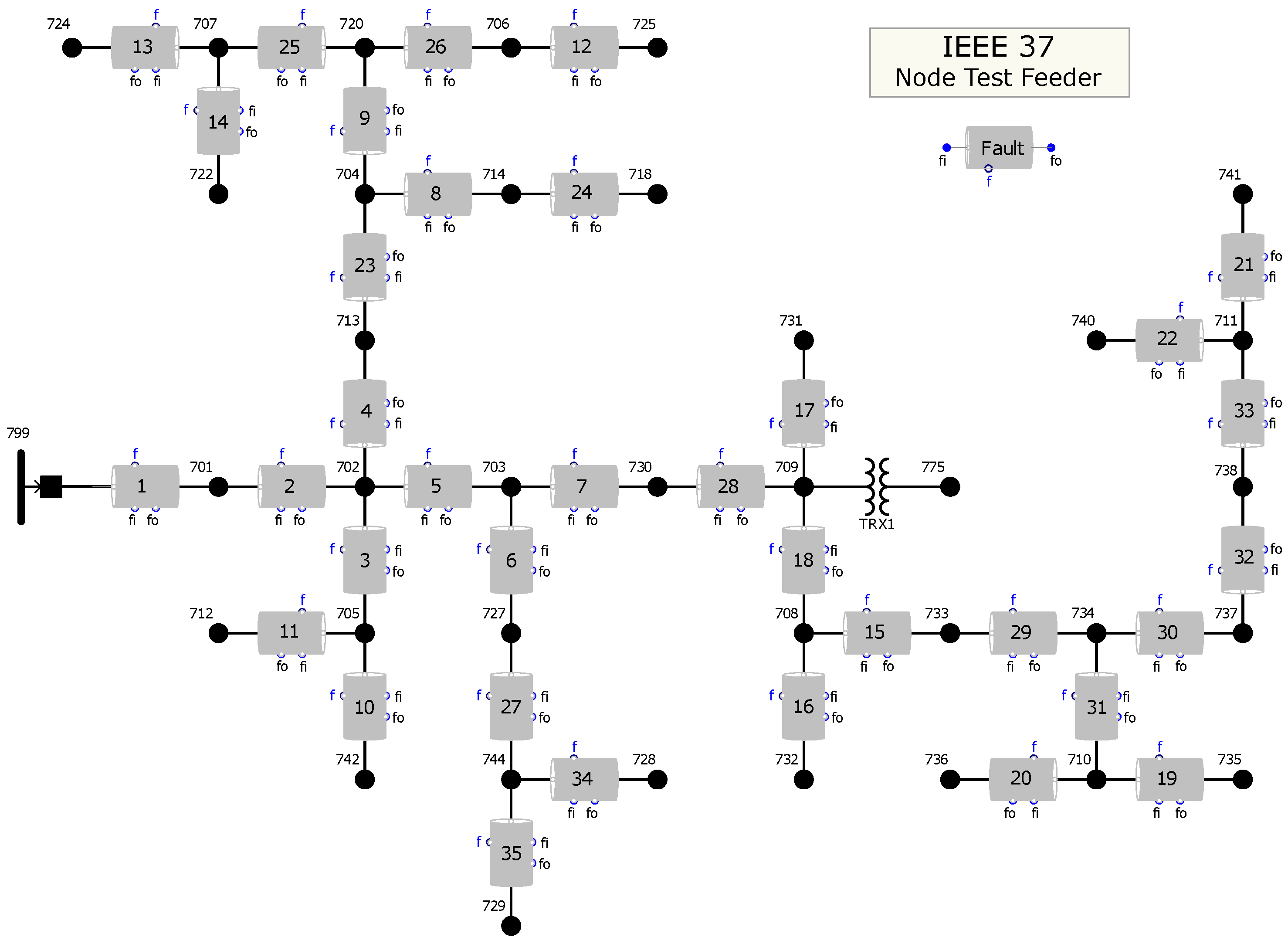
As already discussed in previous sections, this work poses an exhaustive dependency analysis for different impedance-based fault location methods. Obviously, each method has been evaluated individually. However, these results have been done over different testbed networks, making a comparison between their results difficult. In this sense, the IEEE 37 Node Test Feeder [72] (shown in Figure 10) was chosen as the standard underground testbed for this work.

This feeder is one IEEE Node Test Feeders [73] and models a real line located in California. It has an operating voltage of 4.8 kV and its main characteristic (and the reason why it was selected) is that all its line segments are underground (modeled as π-sections characterized by their mutual coupling matrices and their shunt capacities). Moreover, this standardized test network was chosen because of the relative ease with which it could be followed up on with other future location methods. Thus, this line feeder has been implemented in the PSCAD^TM simulation tool [74]. This model provides the main advantage that it can be used to simulate many fault configurations, without subjecting the cabling to extreme conditions typically associated with a fault event which could degrade it.

Thus, a large number of simulations have been done. Each simulation represents a different fault and network configuration (see

Table 2. Fault parameters for the simulation set.

Propriety	Simulation Values	Units
Applied load percentages	0, 25, 50, 75 and 100	%
Fault insertion angle	0, 90, 180 and 270	${}^{\circ }$
Affected fault sections	1, 5, 12, 14, 19, 21, 23, 28 and 34	-
Normalized positions (d)	$0.1$, $0.3$, $0.5$, $0.7$ and $0.9$	$p.u.$
Fault types	single (l-g, one per phase), and three-phase (l-l-l-g)	-
Line-to-sheath resistances ($R_{LS,x}$)	$0.01$, $0.1$, $0.5$, 1, 5, 10 and 100	Ω
Sheath-to-ground resistances ($R_{F,x}$)	$0.01$, $0.1$, $0.5$, 1, 5, 10 and 100	Ω

), reaching a total of 176400 cases, storing their associated measurement.

This simulation set allows us to study the method behavior under different configurations, highlighting their advantages and dependencies in each case.

5. Results

Once the model and its simulation set have been defined, and the resulting information from its execution over PSCAD^TM has been generated, the next step is to analyze the results of applying the six methods selected for this study on it. In this sense, a global evaluation (with the complete simulation set) of them is proposed as the first analysis. Specifically, this analysis has been divided into two stages:

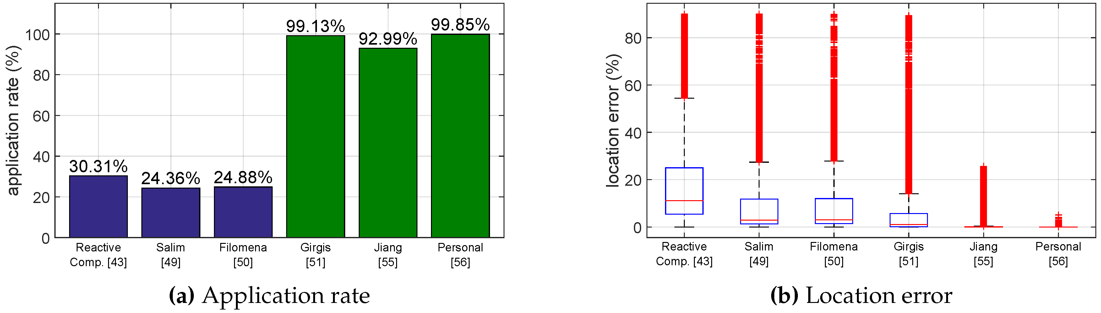
The first stage evaluates the methods’ applicability (when a method obtains a valid result). It allows us to identify when a method offers a valid fault position estimation. This validation criteria considers the limitation of methods (e.g., Reactive Component is only applicable to simple fault) and rejects incoherent results when they are outside of the section ($d<0$ or $d>1$). This analysis is shown in Figure 11a.

In Figure 11a, it is easy to note that one-end methods (the blue ones) have a significantly lower application rate than multi-end methods (the green ones). This fact is mainly caused because these methods fail when the fault appears in segments away from the network header (measurement point). Thus, this problem slightly decreases in the Reactive Component method. This is due to the fact that this method compensates its inability in three-phase faults with its greater applicability under low value load cases. As opposed, multi-end methods provide excellent application rates. However, this comparison must take into account that one-end methods require less information (only measurements at the network header), so that they are at a disadvantage to get a result.

Thus, the Personal et al. method highlights with its highest applicability index, only with a $0.15\%$ of inability cases. This small percentage is associated with three-phase faults and lowers sheath-to-ground resistance values under which the sheath currents are insufficient to apply this method.

In the second stage, the methods’ errors in the estimated position (d) are compared amongst them (see Figure 11b). These errors are represented by box-and-whisker diagrams, it is possible to note how the error dispersion of Jiang et al. and Personal et al. methods are significantly lower than others. Besides, Filomena et al. is the best option of studied one-end methods. This fact is logical because this method is aimed at underground networks. However, many outliers can be observed in this figure. These values mainly correspond to sets of cases where each analyzed method has trouble. Specifically, this fact will be easily noted in the dependency study (Section 5.1, Section 5.2, Section 5.3, Section 5.4, Section 5.5, Section 5.6 and Section 5.7), where parameters such as line-to-sheath resistance, which has a high error when it increases, concentrates many cases on outlier area, especially for one-end methods.

As a summary,

Table 3. Global result summary.

Method	Application	Outliers	Error (%)
	Rate (%)	Rate (%)	Maximum	Average	σ
Reactive comp. [44]	$30.3112$	$6.22043$	$89.9846$	$18.2264$	$1.8242$
Salim et al. [50]	$24.3634$	$12.4811$	$89.9477$	$10.0512$	$1.5182$
Filomena et al. [51]	$24.8753$	$11.9599$	$89.8714$	$9.67601$	$1.41644$
Girgis et al. [52]	$99.1276$	$14.778$	$89.3025$	$7.40104$	$1.52542$
Jiang et al. [56]	$92.9949$	$12.7302$	$25.6445$	$0.275457$	$0.106662$
Personal et al. [57]	$99.8481$	$13.2406$	$5.10298$	$0.00536093$	$0.00526791$

shows all of this information, reflecting both studies numerically. In this table, average, maximum and standard deviation of error values can be compared amongst all studied methods. Thus, after analyzing the results of the complete data set, the following sections will focus on the dependence analysis with the different parameters covered by the simulated cases.

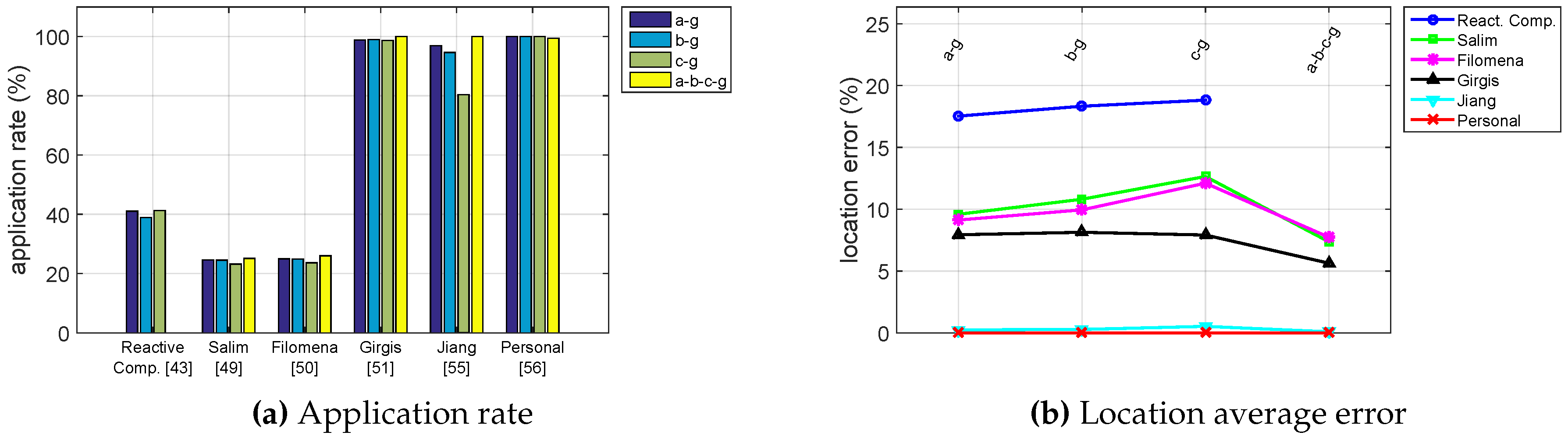
5.1. Fault Type Analysis

In this section, a fault type analysis has been selected as the first study. Following the philosophy of the global analysis, it has also been divided into two stages: an applicability study (see Figure 12a) and an error study (see Figure 12b). Additionally, numerical results of both stages are summarized in

Table A1. Fault type analysis.

Method	Parameter	Application	Error (%)
	Fault Type	Rate (%)	Maximum	Average	$\mathit{\sigma }$
Reactive component  [44]	a-g	$41.03$	$89.96$	$17.53$	$1.85$
	b-g	$38.91$	$89.98$	$18.33$	$1.82$
	c-g	$41.30$	$89.84$	$18.82$	$1.80$
	a-b-c-g	$0.00$	-	-	-
Salim et al. [50]	a-g	$24.61$	$89.07$	$9.59$	$1.46$
	b-g	$24.54$	$89.95$	$10.81$	$1.59$
	c-g	$23.17$	$88.34$	$12.65$	$1.62$
	a-b-c-g	$25.13$	$84.51$	$7.37$	$1.34$
Filomena et al. [51]	a-g	$24.97$	$89.46$	$9.13$	$1.36$
	b-g	$24.88$	$89.13$	$9.95$	$1.41$
	c-g	$23.64$	$89.87$	$12.11$	$1.53$
	a-b-c-g	$26.01$	$89.31$	$7.73$	$1.33$
Girgis et al. [52]	a-g	$98.88$	$88.33$	$7.94$	$1.57$
	b-g	$98.99$	$89.30$	$8.13$	$1.60$
	c-g	$98.64$	$88.56$	$7.92$	$1.56$
	a-b-c-g	$100.00$	$86.21$	$5.64$	$1.35$
Jiang et al. [56]	a-g	$96.93$	$20.04$	$0.25$	$7.82\times {10}^{-2}$
	b-g	$94.62$	$23.43$	$0.28$	$7.67\times {10}^{-2}$
	c-g	$80.43$	$25.64$	$0.53$	$0.19$
	a-b-c-g	$100.00$	$6.67$	$9.27\times {10}^{-2}$	$3.50\times {10}^{-2}$
Personal et al. [57]	a-g	$100.00$	$0.34$	$3.20\times {10}^{-3}$	$1.20\times {10}^{-3}$
	b-g	$100.00$	$0.51$	$3.31\times {10}^{-3}$	$1.56\times {10}^{-3}$
	c-g	$100.00$	$0.98$	$8.19\times {10}^{-3}$	$3.32\times {10}^{-3}$
	a-b-c-g	$99.39$	$5.10$	$6.76\times {10}^{-3}$	$9.81\times {10}^{-3}$

(in the Appendix section).

From this study, it is easy to note the lack of information for three-phase fault in the Reactive Component method. It is due to its inability to estimate a position under this situation. Thus, a reduction in the effectiveness in some of these methods (on the application rate in Jiang et al., and on the location error in Salim et al. and Filomena et al.) for single fault in line c cases is detected. However, this error is not an effect of the fault type. It is due to the fact that this line is unbalanced and has a higher load than others.

In summary, based on the obtained data, it could be argued that the studied methods do not have a strong dependency on the type of fault.

5.2. Insertion Angle Analysis

This analysis evaluates the dependency on the instant when the fault occurs, sweeping values of $0^{\circ }$, ${90}^{\circ }$, ${180}^{\circ }$ and ${270}^{\circ }$. In this sense, Figure 13a shows an applicability study and Figure 13b shows an error study for each method. Additionally, numerical results are summarized in

Table A2. Insertion angle analysis.

Method	Parameter Insertion Angle	Application Rate (%)	Error (%)
			Maximum	Average	$\mathit{\sigma }$
Reactive component [44]	$0^{\circ }$	$29.18$	$89.98$	$18.95$	$1.92$
	${90}^{\circ }$	$31.98$	$89.49$	$16.96$	$1.67$
	${180}^{\circ }$	$28.61$	$89.97$	$19.46$	$1.93$
	${270}^{\circ }$	$31.48$	$89.96$	$17.72$	$1.77$
Salim et al. [50]	$0^{\circ }$	$24.10$	$88.71$	$10.75$	$1.59$
	${90}^{\circ }$	$24.40$	$89.07$	$10.13$	$1.45$
	${180}^{\circ }$	$24.20$	$88.34$	$10.05$	$1.54$
	${270}^{\circ }$	$24.75$	$89.95$	$9.30$	$1.49$
Filomena et al. [51]	$0^{\circ }$	$24.63$	$89.87$	$10.26$	$1.47$
	${90}^{\circ }$	$24.94$	$83.50$	$9.75$	$1.34$
	${180}^{\circ }$	$24.71$	$84.30$	$9.70$	$1.44$
	${270}^{\circ }$	$25.23$	$89.46$	$9.01$	$1.41$
Girgis et al. [52]	$0^{\circ }$	$99.12$	$89.30$	$7.41$	$1.53$
	${90}^{\circ }$	$99.18$	$89.30$	$7.39$	$1.53$
	${180}^{\circ }$	$99.03$	$89.29$	$7.41$	$1.52$
	${270}^{\circ }$	$99.18$	$89.30$	$7.40$	$1.53$
Jiang et al. [56]	$0^{\circ }$	$90.78$	$24.86$	$0.30$	$0.12$
	${90}^{\circ }$	$96.50$	$23.43$	$0.24$	$8.05\times {10}^{-2}$
	${180}^{\circ }$	$90.96$	$25.64$	$0.30$	$0.13$
	${270}^{\circ }$	$93.75$	$20.92$	$0.27$	$9.15\times {10}^{-2}$
Personal et al. [57]	$0^{\circ }$	$99.85$	$5.10$	$6.05\times {10}^{-3}$	$6.44\times {10}^{-3}$
	${90}^{\circ }$	$99.84$	$0.98$	$3.97\times {10}^{-3}$	$2.06\times {10}^{-3}$
	${180}^{\circ }$	$99.85$	$5.05$	$5.99\times {10}^{-3}$	$6.38\times {10}^{-3}$
	${270}^{\circ }$	$99.85$	$3.84$	$5.44\times {10}^{-3}$	$4.96\times {10}^{-3}$

(in the Appendix section).

From this study, it is possible to determine that the insertion angle is not a critical parameter for the estimation of fault position in analyzed methods.

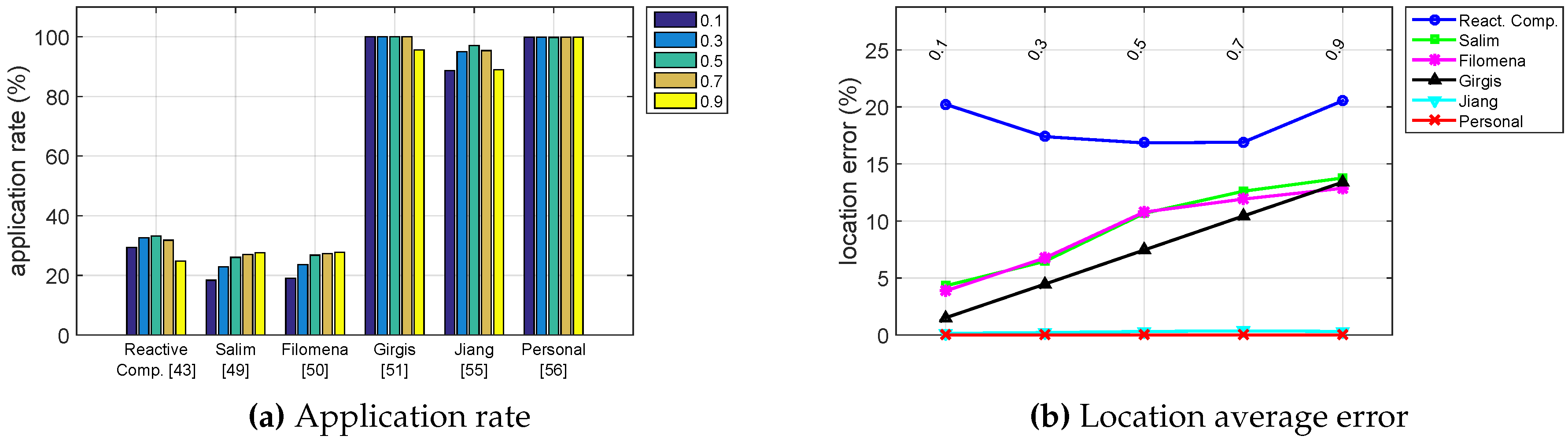
5.3. Normalized Position Analysis

The next analyzed parameter is the normalized position (d) within the line section. In this case, the studied cases sweep the values $0.1$, $0.3$, $0.5$, $0.7$ and $0.9$. From this analysis, Figure 14 is generated, showing the application rates and location errors for each method. Additionally,

Table A3. Normalized position analysis.

Method	Parameter d	Application Rate (%)	Error (%)
			Maximum	Average	$\mathit{\sigma }$
Reactive component [44]	0.1	$29.30$	$89.98$	$20.22$	$2.25$
	0.3	$32.55$	$69.99$	$17.39$	$1.65$
	0.5	$33.19$	$49.98$	$16.84$	$1.37$
	0.7	$31.76$	$69.87$	$16.90$	$1.53$
	0.9	$24.76$	$89.72$	$20.53$	$2.27$
Salim et al. [50]	0.1	$18.36$	$88.25$	$4.32$	$1.14$
	0.3	$22.89$	$67.41$	$6.47$	$0.87$
	0.5	$26.00$	$50.00$	$10.67$	$1.37$
	0.7	$27.00$	$69.52$	$12.61$	$1.66$
	0.9	$27.56$	$89.95$	$13.76$	$1.92$
Filomena et al. [51]	0.1	$19.01$	$84.82$	$3.87$	$0.89$
	0.3	$23.57$	$69.96$	$6.76$	$0.91$
	0.5	$26.76$	$49.99$	$10.78$	$1.35$
	0.7	$27.32$	$69.93$	$11.92$	$1.55$
	0.9	$27.72$	$89.87$	$12.86$	$1.78$
Girgis et al. [52]	0.1	$100.00$	$17.47$	$1.51$	$0.25$
	0.3	$100.00$	$29.65$	$4.47$	$0.76$
	0.5	$100.00$	$49.55$	$7.45$	$1.27$
	0.7	$100.00$	$69.43$	$10.44$	$1.78$
	0.9	$95.64$	$89.30$	$13.40$	$2.34$
Jiang et al. [56]	0.1	$88.62$	$23.43$	$0.15$	$7.10\times {10}^{-2}$
	0.3	$94.99$	$18.85$	$0.22$	$8.60\times {10}^{-2}$
	0.5	$97.05$	$25.64$	$0.31$	$0.12$
	0.7	$95.37$	$23.94$	$0.37$	$0.14$
	0.9	$88.95$	$19.77$	$0.32$	$0.1$
Personal et al. [57]	0.1	$99.89$	$5.10$	$8.81\times {10}^{-3}$	$9.61\times {10}^{-3}$
	0.3	$99.84$	$1.90$	$5.75\times {10}^{-3}$	$4.29\times {10}^{-3}$
	0.5	$99.79$	$0.58$	$2.53\times {10}^{-3}$	$1.31\times {10}^{-3}$
	0.7	$99.84$	$1.31$	$3.88\times {10}^{-3}$	$2.40\times {10}^{-3}$
	0.9	$99.89$	$2.41$	$5.83\times {10}^{-3}$	$4.49\times {10}^{-3}$

(in the Appendix section) summarizes their numerical results.

From this study, it is possible to note that the Reactive Component method performs better in the central portion of the line sections. Salim et al., Filomena et al. and Girgis et al. behavior methods worsen by the increase of d. The Jiang et al. method keeps the error retaining its approximately constant value, but worsens its application rate (about 10%) by moving away from the center of the line sections. Conversely, the Personal et al. method shows a similar behavior for the entire analysis.

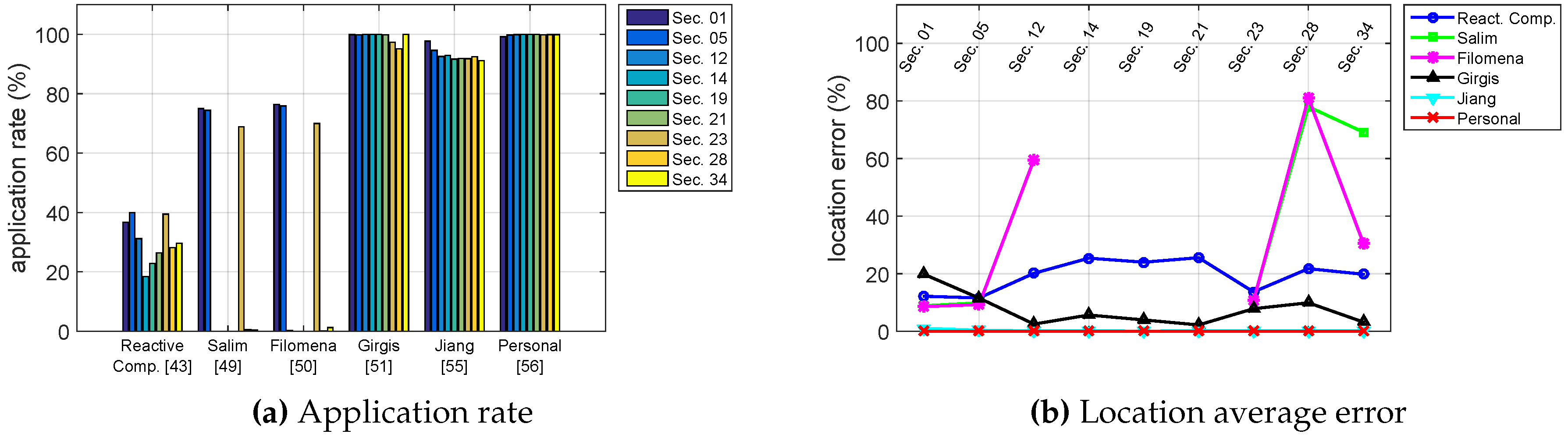
5.4. Affected Fault Section Analysis

In the same direction as the previous section, this study analyzes the behavior of each method result related to the fault position. However, in this case, it is associated with different line sections (see network topology, Figure 10). Specifically, this parameter has been swept for sections 1, 5, 23, 28, 34, 12, 19, 21 and 14 (in order of distance), their results being shown in Figure 15. Thus, numerical results are summarized in

Table A4. Affected fault section analysis.

Method	Parameter Section	Application Rate (%)	Error (%)
			Maximum	Average	$\mathit{\sigma }$
Reactive component [44]	Section 01	$36.71$	$87.97$	$12.19$	$1.54$
	Section 05	$40.01$	$72.82$	$11.60$	$1.44$
	Section 12	$31.20$	$89.96$	$20.16$	$1.92$
	Section 14	$18.46$	$89.91$	$25.41$	$1.71$
	Section 19	$22.86$	$89.97$	$24.01$	$2.05$
	Section 21	$26.40$	$89.98$	$25.58$	$2.17$
	Section 23	$39.44$	$89.69$	$13.69$	$1.56$
	Section 28	$28.12$	$89.33$	$21.77$	$1.80$
	Section 34	$29.60$	$89.84$	$19.83$	$1.69$
Salim et al. [50]	Section 01	$75.03$	$64.08$	$8.90$	$1.36$
	Section 05	$74.43$	$83.02$	$9.91$	$1.49$
	Section 12	$0.00$	-	-	-
	Section 14	$0.00$	-	-	-
	Section 19	$0.00$	-	-	-
	Section 21	$0.00$	-	-	-
	Section 23	$68.91$	$89.95$	$10.62$	$1.53$
	Section 28	$0.50$	$88.25$	$77.99$	$1.12$
	Section 34	$0.39$	$78.73$	$69.18$	$0.59$
Filomena et al. [51]	Section 01	$76.40$	$57.99$	$8.59$	$1.28$
	Section 05	$75.91$	$76.11$	$9.29$	$1.34$
	Section 12	$0.31$	$75.05$	$59.66$	$1.32$
	Section 14	$0.00$	-	-	-
	Section 19	$0.00$	-	-	-
	Section 21	$0.00$	-	-	-
	Section 23	$69.97$	$89.87$	$10.62$	$1.52$
	Section 28	$7.14\times {10}^{-2}$	$84.19$	$80.97$	$0.31$
	Section 34	$1.21$	$89.31$	$30.66$	$2.37$
Girgis et al. [52]	Section 01	$99.93$	$88.87$	$19.80$	$2.25$
	Section 05	$99.85$	$89.30$	$11.55$	$1.91$
	Section 12	$100.00$	$55.25$	$2.52$	$0.73$
	Section 14	$100.00$	$81.66$	$5.67$	$1.35$
	Section 19	$100.00$	$74.39$	$3.97$	$1.07$
	Section 21	$99.86$	$48.31$	$2.22$	$0.60$
	Section 23	$97.40$	$84.16$	$7.86$	$1.50$
	Section 28	$95.11$	$87.09$	$9.92$	$1.68$
	Section 34	$100.00$	$63.83$	$3.23$	$0.85$
Jiang et al. [56]	Section 01	$97.73$	$24.72$	$1.05$	$0.21$
	Section 05	$94.61$	$25.64$	$0.42$	$0.15$
	Section 12	$92.57$	$5.17$	$0.12$	$2.98\times {10}^{-2}$
	Section 14	$92.90$	$6.71$	$0.12$	$4.03\times {10}^{-2}$
	Section 19	$91.68$	$3.26$	$6.06\times {10}^{-2}$	$1.63\times {10}^{-2}$
	Section 21	$91.94$	$18.54$	$0.13$	$6.95\times {10}^{-2}$
	Section 23	$91.85$	$23.43$	$0.17$	$7.02\times {10}^{-2}$
	Section 28	$92.53$	$20.04$	$0.19$	$8.76\times {10}^{-2}$
	Section 34	$91.14$	$17.96$	$0.17$	$7.25\times {10}^{-2}$
Personal et al. [57]	Section 01	$99.20$	$2.37$	$1.59\times {10}^{-2}$	$6.68\times {10}^{-3}$
	Section 05	$99.81$	$5.10$	$1.53\times {10}^{-2}$	$1.35\times {10}^{-2}$
	Section 12	$99.94$	$9.30\times {10}^{-2}$	$6.88\times {10}^{-4}$	$2.57\times {10}^{-4}$
	Section 14	$99.98$	$0.30$	$1.72\times {10}^{-3}$	$7.11\times {10}^{-4}$
	Section 19	$99.96$	$1.31$	$3.99\times {10}^{-3}$	$2.28\times {10}^{-3}$
	Section 21	$99.98$	$0.45$	$1.94\times {10}^{-3}$	$9.38\times {10}^{-4}$
	Section 23	$99.88$	$0.77$	$4.58\times {10}^{-3}$	$2.49\times {10}^{-3}$
	Section 28	$99.94$	$1.36$	$3.19\times {10}^{-3}$	$2.37\times {10}^{-3}$
	Section 34	$99.94$	$0.57$	$9.68\times {10}^{-4}$	$7.46\times {10}^{-4}$

(in the Appendix section).

In this Figure, it is easy to note that the methods of Salim et al. and Filomena et al. exhibit a bad performance, if we turn away from the measuring point (obtaining acceptable results only for the three closest segments). The Reactive Component method is also affected by this parameter, but to a lesser degree. Conversely, as was expected, multi-end methods are not affected by this parameter, because their estimation is directly based on the measurements at both sides of each segment.

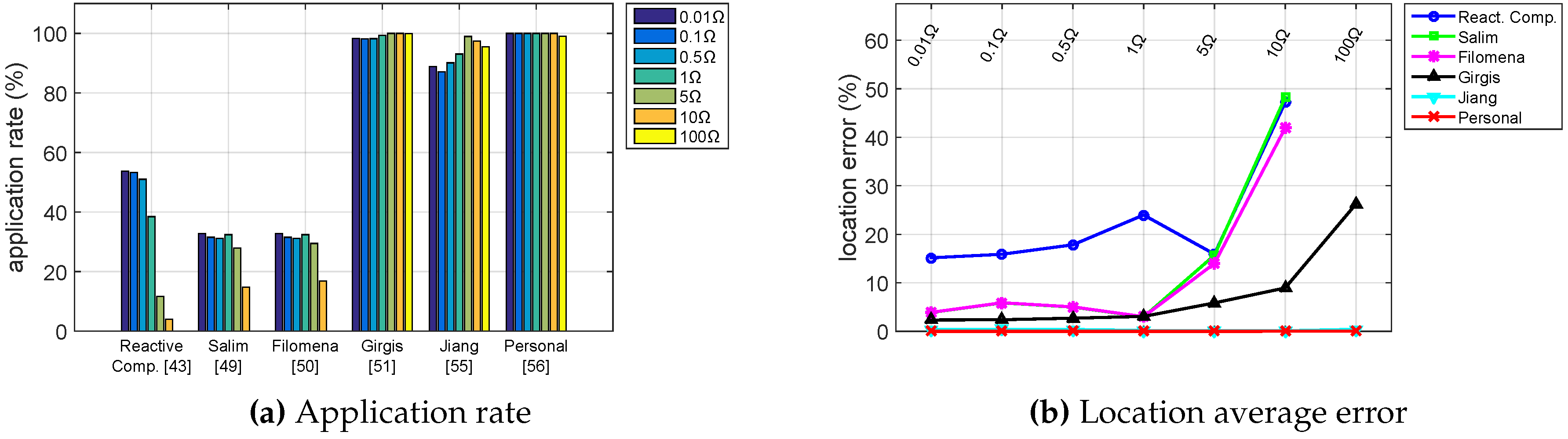
5.5. Line-To-Sheath Resistance Analysis

A typical trouble in fault location methods is their dependency on the fault resistance value. In this work, in order to achieve better characterization of the underground network behavior, this resistance is divided into two parts. Specifically, dependency related to the resistance between the conductor and cable sheath in a fault situation will be analyzed in this section. This line-to-sheath resistance ($R_{LS,x}$) has been swept for 0.01, 0.1, 0.5, 1, 5, 10 and 100 Ω values; their results being shown in Figure 16 and their numerical results in

Table A5. Line-to-sheath resistance analysis.

Method	Parameter ${\mathit{R}}_{\mathit{LS},\mathit{x}}$	Application rate (%)	Error (%)
			Maximum	Average	$\mathit{\sigma }$
Reactive component [44]	$0.01\mathrm{\Omega }$	$53.73$	$89.91$	$15.15$	$1.69$
	$0.1\mathrm{\Omega }$	$53.30$	$89.69$	$15.88$	$1.73$
	$0.5\mathrm{\Omega }$	$50.98$	$89.97$	$17.83$	$1.66$
	$1\mathrm{\Omega }$	$38.47$	$89.98$	$23.98$	$2.14$
	$5\mathrm{\Omega }$	$11.70$	$81.02$	$15.91$	$1.20$
	$10\mathrm{\Omega }$	$4.00$	$88.99$	$47.20$	$1.10$
	$100\mathrm{\Omega }$	$0.00$	-	-	-
Salim et al. [50]	$0.01\mathrm{\Omega }$	$32.77$	$48.31$	$3.89$	$0.63$
	$0.1\mathrm{\Omega }$	$31.55$	$70.57$	$5.85$	$0.99$
	$0.5\mathrm{\Omega }$	$31.14$	$72.54$	$5.00$	$0.91$
	$1\mathrm{\Omega }$	$32.42$	$84.78$	$2.96$	$0.52$
	$5\mathrm{\Omega }$	$27.88$	$72.21$	$15.68$	$0.90$
	$10\mathrm{\Omega }$	$14.79$	$89.95$	$48.25$	$1.31$
	$100\mathrm{\Omega }$	$0.00$	-	-	-
Filomena et al. [51]	$0.01\mathrm{\Omega }$	$32.77$	$48.29$	$3.91$	$0.63$
	$0.1\mathrm{\Omega }$	$31.55$	$70.54$	$5.89$	$0.99$
	$0.5\mathrm{\Omega }$	$31.14$	$72.51$	$5.04$	$0.90$
	$1\mathrm{\Omega }$	$32.42$	$84.82$	$3.02$	$0.51$
	$5\mathrm{\Omega }$	$29.45$	$84.30$	$13.98$	$0.94$
	$10\mathrm{\Omega }$	$16.81$	$89.87$	$41.93$	$1.31$
	$100\mathrm{\Omega }$	$0.00$	-	-	-
Girgis et al. [52]	$0.01\mathrm{\Omega }$	$98.32$	$52.10$	$2.33$	$0.57$
	$0.1\mathrm{\Omega }$	$98.15$	$52.56$	$2.38$	$0.57$
	$0.5\mathrm{\Omega }$	$98.23$	$56.61$	$2.70$	$0.64$
	$1\mathrm{\Omega }$	$99.30$	$60.79$	$3.07$	$0.72$
	$5\mathrm{\Omega }$	$100.00$	$76.13$	$5.85$	$1.17$
	$10\mathrm{\Omega }$	$100.00$	$81.96$	$8.94$	$1.51$
	$100\mathrm{\Omega }$	$99.89$	$89.30$	$26.25$	$2.54$
Jiang et al. [56]	$0.01\mathrm{\Omega }$	$88.85$	$17.96$	$0.38$	$0.13$
	$0.1\mathrm{\Omega }$	$87.07$	$25.64$	$0.43$	$0.17$
	$0.5\mathrm{\Omega }$	$90.11$	$23.94$	$0.38$	$0.12$
	$1\mathrm{\Omega }$	$93.06$	$9.64$	$0.17$	$5.29\times {10}^{-2}$
	$5\mathrm{\Omega }$	$98.92$	$13.01$	$8.51\times {10}^{-2}$	$2.53\times {10}^{-2}$
	$10\mathrm{\Omega }$	$97.44$	$5.13$	$0.10$	$2.74\times {10}^{-2}$
	$100\mathrm{\Omega }$	$95.51$	$20.92$	$0.42$	$0.13$
Personal et al. [57]	$0.01\mathrm{\Omega }$	$99.98$	$0.12$	$1.72\times {10}^{-3}$	$4.43\times {10}^{-4}$
	$0.1\mathrm{\Omega }$	$100.00$	$6.32\times {10}^{-2}$	$1.65\times {10}^{-3}$	$4.10\times {10}^{-4}$
	$0.5\mathrm{\Omega }$	$100.00$	$6.66\times {10}^{-2}$	$1.64\times {10}^{-3}$	$4.15\times {10}^{-4}$
	$1\mathrm{\Omega }$	$100.00$	$0.21$	$1.67\times {10}^{-3}$	$4.69\times {10}^{-4}$
	$5\mathrm{\Omega }$	$100.00$	$2.37$	$2.29\times {10}^{-3}$	$2.75\times {10}^{-3}$
	$10\mathrm{\Omega }$	$99.96$	$1.65$	$2.94\times {10}^{-3}$	$3.26\times {10}^{-3}$
	$100\mathrm{\Omega }$	$99.00$	$5.10$	$2.58\times {10}^{-2}$	$1.31\times {10}^{-2}$

(in the Appendix section).

In this sense, it is easy to note in Figure 16 that the applicability of one-end methods decreases dramatically for high values of this resistance. Additionally, the location error of these methods also gets worse, as was commented in Section 3.1. Conversely, multi-end methods keep their behavior approximately constant, with only Girgis et al. showing an increase in the error for very high values of this parameter.

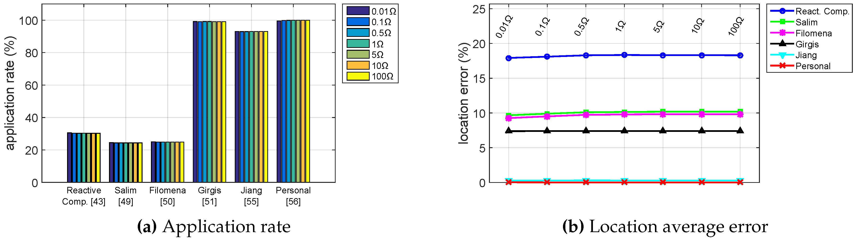
5.6. Sheath-To-Ground Resistance Analysis

This section analyzes the second part of the fault resistance model. It characterizes the resistance which appears between the cable sheath and earth potential in a fault event. As in the previous section, this sheath-to-ground resistance ($R_{F,x}$) has been swept for 0.01, 0.1, 0.5, 1, 5, 10 and 100 Ω values; their results being shown in Figure 17 and their numerical results in

Table A6. Sheath-to-ground resistance analysis.

Method	Parameter ${\mathit{R}}_{\mathit{f},\mathit{x}}$	Application Rate (%)	Error (%)
			Maximum	Average	$\mathit{\sigma }$
Reactive component [44]	$0.01\mathrm{\Omega }$	$30.56$	$89.91$	$17.92$	$1.83$
	$0.1\mathrm{\Omega }$	$30.35$	$89.98$	$18.10$	$1.83$
	$0.5\mathrm{\Omega }$	$30.27$	$89.93$	$18.30$	$1.83$
	$1\mathrm{\Omega }$	$30.28$	$89.97$	$18.35$	$1.83$
	$5\mathrm{\Omega }$	$30.25$	$89.92$	$18.31$	$1.82$
	$10\mathrm{\Omega }$	$30.23$	$89.92$	$18.31$	$1.82$
	$100\mathrm{\Omega }$	$30.23$	$89.93$	$18.30$	$1.82$
Salim et al. [50]	$0.01\mathrm{\Omega }$	$24.48$	$89.48$	$9.67$	$1.49$
	$0.1\mathrm{\Omega }$	$24.36$	$89.78$	$9.89$	$1.51$
	$0.5\mathrm{\Omega }$	$24.33$	$89.90$	$10.10$	$1.52$
	$1\mathrm{\Omega }$	$24.34$	$89.93$	$10.15$	$1.52$
	$5\mathrm{\Omega }$	$24.34$	$89.94$	$10.18$	$1.53$
	$10\mathrm{\Omega }$	$24.34$	$89.95$	$10.18$	$1.53$
	$100\mathrm{\Omega }$	$24.35$	$89.95$	$10.19$	$1.53$
Filomena et al. [51]	$0.01\mathrm{\Omega }$	$24.98$	$89.42$	$9.27$	$1.38$
	$0.1\mathrm{\Omega }$	$24.87$	$89.71$	$9.51$	$1.40$
	$0.5\mathrm{\Omega }$	$24.85$	$89.83$	$9.73$	$1.42$
	$1\mathrm{\Omega }$	$24.86$	$89.85$	$9.78$	$1.42$
	$5\mathrm{\Omega }$	$24.86$	$89.87$	$9.81$	$1.43$
	$10\mathrm{\Omega }$	$24.85$	$89.87$	$9.81$	$1.43$
	$100\mathrm{\Omega }$	$24.86$	$89.87$	$9.82$	$1.43$
Girgis et al. [52]	$0.01\mathrm{\Omega }$	$99.15$	$89.30$	$7.38$	$1.52$
	$0.1\mathrm{\Omega }$	$99.12$	$89.30$	$7.39$	$1.53$
	$0.5\mathrm{\Omega }$	$99.13$	$89.30$	$7.40$	$1.53$
	$1\mathrm{\Omega }$	$99.13$	$89.30$	$7.41$	$1.53$
	$5\mathrm{\Omega }$	$99.12$	$89.30$	$7.41$	$1.53$
	$10\mathrm{\Omega }$	$99.12$	$89.30$	$7.41$	$1.53$
	$100\mathrm{\Omega }$	$99.12$	$89.30$	$7.41$	$1.53$
Jiang et al. [56]	$0.01\mathrm{\Omega }$	$93.01$	$23.43$	$0.25$	$9.41\times {10}^{-2}$
	$0.1\mathrm{\Omega }$	$92.97$	$23.94$	$0.28$	$0.10$
	$0.5\mathrm{\Omega }$	$92.94$	$23.86$	$0.28$	$0.11$
	$1\mathrm{\Omega }$	$93.00$	$24.72$	$0.28$	$0.11$
	$5\mathrm{\Omega }$	$93.01$	$25.38$	$0.28$	$0.11$
	$10\mathrm{\Omega }$	$93.02$	$25.51$	$0.28$	$0.11$
	$100\mathrm{\Omega }$	$93.01$	$25.64$	$0.28$	$0.11$
Personal et al. [57]	$0.01\mathrm{\Omega }$	$99.50$	$2.37$	$1.47\times {10}^{-2}$	$5.93\times {10}^{-3}$
	$0.1\mathrm{\Omega }$	$99.86$	$5.10$	$4.77\times {10}^{-3}$	$6.19\times {10}^{-3}$
	$0.5\mathrm{\Omega }$	$99.90$	$4.00$	$3.85\times {10}^{-3}$	$5.22\times {10}^{-3}$
	$1\mathrm{\Omega }$	$99.92$	$3.86$	$3.68\times {10}^{-3}$	$4.97\times {10}^{-3}$
	$5\mathrm{\Omega }$	$99.92$	$3.74$	$3.53\times {10}^{-3}$	$4.78\times {10}^{-3}$
	$10\mathrm{\Omega }$	$99.92$	$3.72$	$3.51\times {10}^{-3}$	$4.75\times {10}^{-3}$
	$100\mathrm{\Omega }$	$99.92$	$3.71$	$3.49\times {10}^{-3}$	$4.73\times {10}^{-3}$

(in the Appendix section).

As can be seen in both Figures, it is not only the behavior of the six studied methods that is affected by this parameter. This fact can be explained because the sheath acts as a better way (with less resistance) for the fault current than ground potential, only appreciating small variations for very small values of this parameter.

5.7. Applied Load Percentages Analysis

The last study is related to the network load level. For this study, several percentages of a load factor have been applied over the network. Specifically, this parameter has been swept for $0\%$, $25\%$, $50\%$, $75\%$ and $100\%$ of the load associated with this network. Following the philosophy of previous sections, it has also been divided into two stages: an applicability study (see Figure 18a) and an error study (see Figure 18b). Additionally, numerical results of both stages are summarized in

Table A7. Applied load percentage analysis.

Method	Parameter Load	Application Rate (%)	Error (%)
			Maximum	Average	$\mathit{\sigma }$
Reactive component [44]	$0\%$	$50.81$	$88.99$	$11.76$	$1.21$
	$25\%$	$29.89$	$89.91$	$19.57$	$1.75$
	$50\%$	$24.98$	$89.98$	$22.04$	$2.02$
	$75\%$	$23.22$	$89.84$	$22.97$	$2.11$
	$100\%$	$22.65$	$89.96$	$21.90$	$2.08$
Salim et al. [50]	$0\%$	$26.08$	$88.25$	$7.77$	$1.37$
	$25\%$	$24.32$	$89.07$	$10.77$	$1.63$
	$50\%$	$23.78$	$89.95$	$11.00$	$1.57$
	$75\%$	$23.84$	$87.20$	$10.47$	$1.47$
	$100\%$	$23.80$	$85.99$	$10.45$	$1.53$
Filomena et al. [51]	$0\%$	$26.72$	$50.97$	$6.59$	$1.05$
	$25\%$	$24.77$	$84.82$	$10.21$	$1.51$
	$50\%$	$24.07$	$89.87$	$10.53$	$1.45$
	$75\%$	$24.46$	$89.31$	$10.90$	$1.52$
	$100\%$	$24.36$	$89.46$	$10.45$	$1.48$
Girgis et al. [52]	$0\%$	$100.00$	$15.97$	$0.17$	$6.86\times {10}^{-2}$
	$25\%$	$99.47$	$86.48$	$5.85$	$1.26$
	$50\%$	$98.78$	$88.64$	$8.58$	$1.58$
	$75\%$	$98.68$	$89.13$	$10.52$	$1.77$
	$100\%$	$98.71$	$89.30$	$11.99$	$1.90$
Jiang et al. [56]	$0\%$	$96.46$	$20.92$	$0.16$	$8.16\times {10}^{-2}$
	$25\%$	$91.26$	$25.64$	$0.32$	$0.14$
	$50\%$	$90.49$	$24.72$	$0.31$	$0.12$
	$75\%$	$92.80$	$18.86$	$0.30$	$0.10$
	$100\%$	$93.97$	$14.28$	$0.29$	$8.65\times {10}^{-2}$
Personal et al. [57]	$0\%$	$99.26$	$5.10$	$7.43\times {10}^{-3}$	$1.09\times {10}^{-2}$
	$25\%$	$99.99$	$0.50$	$3.51\times {10}^{-3}$	$1.51\times {10}^{-3}$
	$50\%$	$99.99$	$0.75$	$4.74\times {10}^{-3}$	$2.13\times {10}^{-3}$
	$75\%$	$100.00$	$0.89$	$5.38\times {10}^{-3}$	$2.52\times {10}^{-3}$
	$100\%$	$100.00$	$0.98$	$5.75\times {10}^{-3}$	$2.78\times {10}^{-3}$

(in the Appendix section).

In this sense, on the one hand, the Reactive Component method is highlighted by its strong dependency on this parameter. This fact occurs because, as already discussed above, this method assumes that overall registered current is completely due to the fault event (dismissing the load effects). Obviously, it operates significantly worse when this load current is not negligible. Thus, the behavior of the other one-end methods remains approximately stable under changes in this parameter. In the other one-end methods, their behavior remains approximately stable with this parameter. On the other hand, regarding the multi-end methods, Jiang et al. and Personal et al. show a fairly stable behavior. This fact is logical, due to their multi-end philosophy (with measurements at both ends of the line section). However, the Girgis et al. method does not have this characteristic, increasing its error with this parameter.

6. Conclusions

Throughout this paper, the needs for better strategies on operation and planning tasks are highlighted as a key factor in SG networks. In this sense, fault location is a cornerstone of the OMS, allowing this system to identify the fault position and mitigate its consequences.

In this paper, a comparative review of different fault location techniques has been done. Specifically, this study is focused on impedance-based methods because they are more in line with typical instrumentation deployed in the distribution systems, distinguishing two sets of methods. On the one had, one-end methods have been analyzed, the main advantage being less deployment needs (only one measuring point). However, they have higher errors than the second set of methods, and have the significant drawback of not being compatible with DG scenarios. Reactive Component, Salim et al. and Filomena et al. methods have been chosen as relevant examples for their evaluation. On the other hand, multi-end methods have also been studied. This set provides better results than one-end methods. However, this fact mainly occurs because they are supported by a greater measurement infrastructure, which is significantly more expensive than one-end method deployments. Additionally, multi-end methods are compatible with DG scenarios, thus being a perfect solution for SG networks. For this second set, the methods of Girgis et al., Jiang et al. and Personal et al. have been the chosen methods as relevant examples for their evaluation.

In this sense, these six chosen methods have been widely tested, studying their dependencies under different conditions. All of these studies have been based on an implementation over PSCAD^TM of a standard test network (the IEEE 37 Node Test Feeder). The use of a common testbed has allowed this study to coherently compare the different method results, beyond typical individual analyses in these methods. Thus, for these studies, the multi-end methods of Personal et al. and Jiang et al. are the best options due to their excellent results. However, Filomena et al. is the best option of the analyzed one-end method, being a good option for underground networks where a multi-end deployment is not possible.

References

1. Farhangi, H. The path of the smart grid. IEEE Power Energy Mag. 2010, 8, 18–28. [Google Scholar] [CrossRef]
2. Kezunovic, M.; McCalley, J.D.; Overbye, T.J. Smart Grids and Beyond: Achieving the Full Potential of Electricity Systems. Proc. IEEE 2012, 100, 1329–1341. [Google Scholar] [CrossRef]
3. Ardito, L.; Procaccianti, G.; Menga, G.; Morisio, M. Smart Grid Technologies in Europe: An Overview. Energies 2013, 6, 251–281. [Google Scholar] [CrossRef]
4. Personal, E.; Guerrero, J.I.; Garcia, A.; Peña, M.; Leon, C. Key performance indicators: A useful tool to assess Smart Grid goals. Energy 2014, 76, 976–988. [Google Scholar] [CrossRef]
5. Grid 2030—A National Vision for Electricity’s Second 100 Years; Office of Electricity Delivery and Energy Reliability, US Departament of Energy: Washington, DC, USA, 2003.
6. Song, G.; Chen, H.; Guo, B. A Layered Fault Tree Model for Reliability Evaluation of Smart Grids. Energies 2014, 7, 4835–4857. [Google Scholar] [CrossRef]
7. Ackermann, T.; Andersson, G.; Söder, L. Distributed generation: A definition. Electr. Power Syst. Res. 2001, 57, 195–204. [Google Scholar] [CrossRef]
8. Ferreira, H.L.; Garde, R.; Fulli, G.; Kling, W.; Lopes, J.P. Characterisation of electrical energy storage technologies. Energy 2013, 53, 288–298. [Google Scholar] [CrossRef]
9. Palensky, P.; Dietrich, D. Demand Side Management: Demand Response, Intelligent Energy Systems, and Smart Loads. IEEE Trans. Ind. Inform. 2011, 7, 381–388. [Google Scholar] [CrossRef]
10. Shen, J.; Jiang, C.; Li, B. Controllable Load Management Approaches in Smart Grids. Energies 2015, 8, 11187–11202. [Google Scholar] [CrossRef]
11. Lasseter, R.H. Smart Distribution: Coupled Microgrids. Proc. IEEE 2011, 99, 1074–1082. [Google Scholar] [CrossRef]
12. Moslehi, K.; Kumar, R. A Reliability Perspective of the Smart Grid. IEEE Trans. Smart Grid 2010, 1, 57–64. [Google Scholar] [CrossRef]
13. Amin, S.M.; Giacomoni, A.M. Smart Grid—Safe, Secure, Self-Healing. IEEE Power Energy Mag. 2012, 10, 33–40. [Google Scholar] [CrossRef]
14. Hwang, I.; Kim, S.; Kim, Y.; Seah, C.E. A Survey of Fault Detection, Isolation, and Reconfiguration Methods. IEEE Trans. Control Syst. Technol. 2010, 18, 636–653. [Google Scholar] [CrossRef]
15. Das, R.; Madani, V.; Aminifar, F.; McDonald, J.; Venkata, S.S.; Novosel, D.; Bose, A.; Shahidehpour, M. Distribution Automation Strategies: Evolution of Technologies and the Business Case. IEEE Trans. Smart Grid 2015, 6, 2166–2175. [Google Scholar] [CrossRef]
16. Rahmati, A.; Adhami, R. A Fault Detection and Classification Technique Based on Sequential Components. IEEE Trans. Ind. Appl. 2014, 50, 4202–4209. [Google Scholar] [CrossRef]
17. Sachdev, M.; Baribeau, M. A New Algorithm for Digital Impedance Relays. IEEE Trans. Power Appar. Syst. 1979, PAS-98, 2232–2240. [Google Scholar] [CrossRef]
18. Sheng, Y.; Rovnyak, S. Decision Tree-Based Methodology for High Impedance Fault Detection. IEEE Trans. Power Deliv. 2004, 19, 533–536. [Google Scholar] [CrossRef]
19. Liang, F.; Jeyasurya, B. Transmission Line Distance Protection Using Wavelet Transform Algorithm. IEEE Trans. Power Deliv. 2004, 19, 545–553. [Google Scholar] [CrossRef]
20. Adu, T. An accurate fault classification technique for power system monitoring devices. IEEE Trans. Power Deliv. 2002, 17, 684–690. [Google Scholar] [CrossRef]
21. Perez, F.; Orduña, E.; Guidi, G. Adaptive wavelets applied to fault classification on transmission lines. IET Gener. Transm. Distrib. 2011, 5, 694–702. [Google Scholar] [CrossRef]
22. Silva, K.; Souza, B.; Brito, N. Fault Detection and Classification in Transmission Lines Based on Wavelet Transform and ANN. IEEE Trans. Power Deliv. 2006, 21, 2058–2063. [Google Scholar] [CrossRef]
23. Yadav, A.; Swetapadma, A. Enhancing the performance of transmission line directional relaying, fault classification and fault location schemes using fuzzy inference system. IET Gener. Transm. Distrib. 2015, 9, 580–591. [Google Scholar] [CrossRef]
24. Jamehbozorg, A.; Shahrtash, S.M. A Decision-Tree-Based Method for Fault Classification in Single-Circuit Transmission Lines. IEEE Trans. Power Deliv. 2010, 25, 2190–2196. [Google Scholar] [CrossRef]
25. Jiang, J.A.; Chuang, C.L.; Wang, Y.C.; Hung, C.H.; Wang, J.Y.; Lee, C.H.; Hsiao, Y.T. A Hybrid Framework for Fault Detection, Classification, and Location—Part I: Concept, Structure, and Methodology. IEEE Trans. Power Deliv. 2011, 26, 1988–1998. [Google Scholar] [CrossRef]
26. IEEE Std. C37.114-2014. IEEE Guide for Determining Fault Location on AC Transmission and Distribution Lines; IEEE: New York, NY, USA, 2015.
27. Brahma, S.M. Fault Location in Power Distribution System With Penetration of Distributed Generation. IEEE Trans. Power Deliv. 2011, 26, 1545–1553. [Google Scholar] [CrossRef]
28. Cuadra, L.; Salcedo-Sanz, S.; Del Ser, J.; Jimenez-Fernandez, S.; Geem, Z. A Critical Review of Robustness in Power Grids Using Complex Networks Concepts. Energies 2015, 8, 9211–9265. [Google Scholar] [CrossRef] [Green Version]
29. Kezunovic, M. Smart Fault Location for Smart Grids. IEEE Trans. Smart Grid 2011, 2, 11–22. [Google Scholar] [CrossRef]
30. Bo, Z.; Weller, G.; Redfern, M. Accurate fault location technique for distribution system using fault-generated high-frequency transient voltage signals. IEE Proc. Gener. Transm. Distrib. 1999, 146, 73–79. [Google Scholar] [CrossRef]
31. Dommel, H.; Michels, J. High-speed relaying using traveling wave transient analysis. IEEE Trans. Power Appar. Syst. 1978, 97, 1011. [Google Scholar]
32. McLaren, P.; Rajendra, S. Travelling-Wave Techniques Applied to the Protection of Teed Circuits: Principle of Travelling-Wave Techniques. IEEE Trans. Power Appar. Syst. 1985, PAS-104, 3544–3550. [Google Scholar] [CrossRef]
33. Magnago, F.; Abur, A. Fault location using wavelets. IEEE Trans. Power Deliv. 1998, 13, 1475–1480. [Google Scholar] [CrossRef]
34. Jafarian, P.; Sanaye-Pasand, M. A Traveling-Wave-Based Protection Technique Using Wavelet/PCA Analysis. IEEE Trans. Power Deliv. 2010, 25, 588–599. [Google Scholar] [CrossRef]
35. Mosavi, M.R.; Tabatabaei, A. Traveling-Wave Fault Location Techniques in Power System Based on Wavelet Analysis and Neural Network Using GPS Timing. Wirel. Pers. Commun. 2015, 86, 835–850. [Google Scholar] [CrossRef]
36. Livani, H.; Evrenosoglu, C. A machine learning and wavelet-based fault location method for hybrid transmission lines. IEEE Trans. Smart Grid 2014, 5, 51–59. [Google Scholar] [CrossRef]
37. Dutta, P.; Esmaeilian, A.; Kezunovic, M. Transmission-Line Fault Analysis Using Synchronized Sampling. IEEE Trans. Power Deliv. 2014, 29, 942–950. [Google Scholar] [CrossRef]
38. Kulkarni, S.; Santoso, S. Time-Domain Algorithm for Locating Evolving Faults. IEEE Trans. Smart Grid 2012, 3, 1584–1593. [Google Scholar] [CrossRef]
39. Esmaeilian, A.; Popovic, T.; Kezunovic, M. Transmission line relay mis-operation detection based on time-synchronized field data. Electr. Power Syst. Res. 2015, 125, 174–183. [Google Scholar] [CrossRef]
40. Mallat, S. A theory for multiresolution signal decomposition: The wavelet representation. IEEE Trans. Pattern Anal. Mach. Intell. 1989, 11, 674–693. [Google Scholar] [CrossRef]
41. Da Silva, A.P.A.; Lima, A.C.; Souza, S.M. Fault location on transmission lines using complex-domain neural networks. Int. J. Electr. Power Energy Syst. 2012, 43, 720–727. [Google Scholar] [CrossRef]
42. Rafinia, A.; Moshtagh, J. A new approach to fault location in three-phase underground distribution system using combination of wavelet analysis with ANN and FLS. Int. J. Electr. Power Energy Syst. 2014, 55, 261–274. [Google Scholar] [CrossRef]
43. Sadeh, J.; Afradi, H. A new and accurate fault location algorithm for combined transmission lines using Adaptive Network-Based Fuzzy Inference System. Elec. Power Syst. Res. 2009, 79, 1538–1545. [Google Scholar] [CrossRef]
44. Van, C. Warrington, A.R. Protective Relays; Springer Science: New York, NY, USA, 1968. [Google Scholar]
45. Girgis, A.; Fallon, C.; Lubkeman, D. A fault location technique for rural distribution feeders. IEEE Trans. Ind. Appl. 1993, 29, 1170–1175. [Google Scholar] [CrossRef]
46. Das, R.; Sachdev, M.; Sidhu, T. A fault locator for radial subtransmission and distribution lines. In Proceedings of the Power Engineering Society Summer Meeting, Seattle, WA, USA, 16–20 July 2000.
47. Novosel, D.; Hart, D.; Hu, Y.; Myllymaki, J. System for Locating Faults and Estimating Fault Resistance in Distribution Networks with Tapped Loads. U.S. Patent 5839093A, 17 November 1998. [Google Scholar]
48. Lee, S.J.; Choi, M.S.; Kang, S.H.; Jin, B.G.; Lee, D.S.; Ahn, B.S.; Yoon, N.S.; Kim, H.Y.; Wee, S.B. An Intelligent and Efficient Fault Location and Diagnosis Scheme for Radial Distribution Systems. IEEE Trans. Power Deliv. 2004, 19, 524–532. [Google Scholar] [CrossRef]
49. Choi, M.S.; Lee, S.J.; Lee, D.S.; Jin, B.G. A New Fault Location Algorithm Using Direct Circuit Analysis for Distribution Systems. IEEE Trans. Power Deliv. 2004, 19, 35–41. [Google Scholar] [CrossRef]
50. Salim, R.; Resener, M.; Filomena, A.; Rezende Caino de Oliveira, K.; Bretas, A. Extended Fault-Location Formulation for Power Distribution Systems. IEEE Trans. Power Deliv. 2009, 24, 508–516. [Google Scholar] [CrossRef]
51. Filomena, A.; Resener, M.; Salim, R.; Bretas, A. Fault Location for Underground Distribution Feeders: An Extended Impedance-Based Formulation with Capacitive Current Compensation. Int. J. Electr. Power Energy Syst. 2009, 31, 489–496. [Google Scholar] [CrossRef]
52. Girgis, A.; Hart, D.; Peterson, W. A new fault location technique for two- and three-terminal lines. IEEE Trans. Power Deliv. 1992, 7, 98–107. [Google Scholar] [CrossRef]
53. Liu, C.W.; Lin, T.C.; Yu, C.S.; Yang, J.Z. A Fault Location Technique for Two-Terminal Multisection Compound Transmission Lines Using Synchronized Phasor Measurements. IEEE Trans. Smart Grid 2012, 3, 113–121. [Google Scholar] [CrossRef]
54. Lin, T.C.; Lin, P.Y.; Liu, C.W. An Algorithm for Locating Faults in Three-Terminal Multisection Nonhomogeneous Transmission Lines Using Synchrophasor Measurements. IEEE Trans. Smart Grid 2014, 5, 38–50. [Google Scholar] [CrossRef]
55. Terzija, V.; Radojevic, Z.M.; Preston, G. Flexible Synchronized Measurement Technology-Based Fault Locator. IEEE Trans. Smart Grid 2015, 6, 866–873. [Google Scholar] [CrossRef]
56. Jiang, Q.; Wang, B.; Li, X. An Efficient PMU-Based Fault-Location Technique for Multiterminal Transmission Lines. IEEE Trans. Power Deliv. 2014, 29, 1675–1682. [Google Scholar] [CrossRef]
57. Personal, E. Sistema para Localización de Faltas en Líneas Subterráneas de Distribución Eléctrica de Media Tensión, Mediante una Red Distribuida de Sensores de Corriente. Ph.D. Thesis, University of Seville, Seville, Spain, 2015. [Google Scholar]
58. Biscaro, A.A.P.; Pereira, R.A.F.; Kezunovic, M.; Mantovani, J.R.S. Integrated Fault Location and Power-Quality Analysis in Electric Power Distribution Systems. IEEE Trans. Power Deliv. 2016, 31, 428–436. [Google Scholar] [CrossRef]
59. Mirzaei, M.; Ab Kadir, M.Z.A.; Moazami, E.; Hizam, H. Review of fault location methods for distribution power system. Aust. J. Basic Appl. Sci. 2009, 3, 2670–2676. [Google Scholar]
60. Borghetti, A.; Bosetti, M.; Di Silvestro, M.; Nucci, C.A.; Paolone, M.; Peretto, L.; Scala, E.; Tinarelli, R. Assessment of Fault Location in Power Distribution Networks. Electr. Power Qual. Util. 2007, 13, 33–41. [Google Scholar]
61. Murari Mohan, S.; Ratan, D.; Verho, P.; Novosel, D. Review of fault location techniques for distribution systems. In Proceedings of the Power Systems and Communications Instruments for the Future, Beijing, China, 23–27 September 2002.
62. Mora-Florez, J.; Melendez, J.; Carrillo-Caicedo, G. Comparison of impedance based fault location methods for power distribution systems. Electr. Power Syst. Res. 2008, 78, 657–666. [Google Scholar] [CrossRef]
63. Al-Mohammed, A.H.; Abido, M.A. Fault Location Based on Synchronized Measurements: A Comprehensive Survey. Sci. World J. 2014, 2014, 845307. [Google Scholar] [CrossRef] [PubMed]
64. De Almeida, M.; Costa, F.; Xavier-de Souza, S.; Santana, F. Optimal placement of faulted circuit indicators in power distribution systems. Electr. Power Syst. Res. 2011, 81, 699–706. [Google Scholar] [CrossRef]
65. Lotfifard, S.; Kezunovic, M.; Mousavi, M.J. A Systematic Approach for Ranking Distribution Systems Fault Location Algorithms and Eliminating False Estimates. IEEE Trans. Power Deliv. 2013, 28, 285–293. [Google Scholar] [CrossRef]
66. Mora-Florez, J.; Barrera-Nuez, V.; Carrillo-Caicedo, G. Fault Location in Power Distribution Systems Using a Learning Algorithm for Multivariable Data Analysis. IEEE Trans. Power Deliv. 2007, 22, 1715–1721. [Google Scholar] [CrossRef]
67. Salim, R.; de Oliveira, K.; Filomena, A.; Resener, M.; Bretas, A. Hybrid Fault Diagnosis Scheme Implementation for Power Distribution Systems Automation. IEEE Trans. Power Deliv. 2008, 23, 1846–1856. [Google Scholar] [CrossRef]
68. Mora-Florez, J.; Morales-Espana, G.; Perez-Londono, S. Learning-based strategy for reducing the multiple estimation problem of fault zone location in radial power systems. IET Gener. Transm. Distrib. 2009, 3, 346–356. [Google Scholar] [CrossRef]
69. Zhang, Z.; Gong, S.; Dimitrovski, A.D.; Li, H. Time Synchronization Attack in Smart Grid: Impact and Analysis. IEEE Trans. Smart Grid 2013, 4, 87–98. [Google Scholar] [CrossRef]
70. Terzija, V.; Valverde, G.; Cai, D.; Regulski, P.; Madani, V.; Fitch, J.; Skok, S.; Begovic, M.M.; Phadke, A. Wide-Area Monitoring, Protection, and Control of Future Electric Power Networks. Proc. IEEE 2011, 99, 80–93. [Google Scholar] [CrossRef]
71. Phadke, A.; Thorp, J. Synchronized Phasor Measurements and Their Applications; Springer: New York, NY, USA, 2008. [Google Scholar]
72. IEEE 37-Node Test Feeder Report. Distribution System Analysis Subcommittee. Available online: http://ewh.ieee.org/soc/pes/dsacom/testfeeders/ (accessed on 29 November 2016).
73. Kersting, W. Radial distribution test feeders. IEEE Trans. Power Syst. 1991, 6, 975–985. [Google Scholar] [CrossRef]
74. PSCAD User’s Guide; Manitoba HVDC Research Centre: Winnipeg, MB, Canada, 2010.
Figure 1. Brief description of the self-healing process.
Energies 09 01022 g001
Figure 2. Simplified line model for general one-end methods.
Energies 09 01022 g002
Figure 3. Simplified model of a faulted section in the Salim et al. method [50].
Energies 09 01022 g003
Figure 4. Simplified model of an underground faulted section in the Filomena et al. method [51].
Energies 09 01022 g004
Figure 5. Simplified line model for general multi-end methods.
Energies 09 01022 g005
Figure 6. Simplified line model for the Girgis et al. [52] method.
Energies 09 01022 g006
Figure 7. Simplified model of section in the Jiang et al. method [56].
Energies 09 01022 g007
Figure 8. Line section model for the Personal et al. [57] method.
Energies 09 01022 g008
Figure 9. Proposed deployment for the Personal et al. [57] method.
Energies 09 01022 g009
Figure 10. Testbed network for comparative (IEEE 37 Node Test Feeder).
Energies 09 01022 g010
Figure 11. Global analysis results.
Energies 09 01022 g011
Figure 12. Fault type analysis.
Energies 09 01022 g012
Figure 13. Insertion angle analysis.
Energies 09 01022 g013
Figure 14. Normalized position analysis.
Energies 09 01022 g014
Figure 15. Affected fault section analysis.
Energies 09 01022 g015
Figure 16. Line-to-sheath resistance analysis.
Energies 09 01022 g016
Figure 17. Sheath-to-ground resistance analysis.
Energies 09 01022 g017
Figure 18. Applied load percentage analysis.
Energies 09 01022 g018