A Flexible Ramping Capacity Model for Generation Scheduling with High Levels of Wind Energy Penetration

Abstract

The penetration level of renewable generation has increased significantly in recent years, which has led to operational concerns associated with the system ramping capability. Here, we propose the flexible ramping capacity (FRC) model, which considers the practical ramping capability of generation resources as well as the uncertainty in net load. The FRC model also incorporates the demand curve of the ramping capacity, which represents the hourly economic value of the ramping capacity. The model is formulated mathematically using ramp constraints, which are incorporated into unit commitment (UC) and economic dispatch (ED) processes. Simulations are carried out using a 10-unit system to compare the FRC model with conventional methods. We show that the FRC method can improve reliability and reduce expected operating costs. The simulation results also show that, by using the FRC model, system reliability can be satisfied at high wind power generation levels while achieving economic efficiency.

1. Introduction

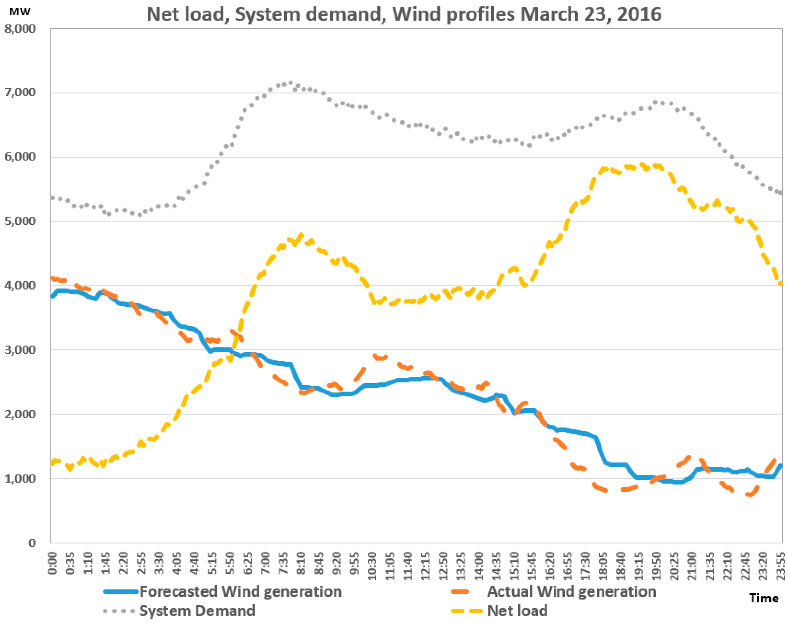
The penetration of intermittent renewable generation resources has increased significantly in recent years, which has led to increased variability of the system net load. This has resulted in challenges for independent system operators (ISOs), including frequency control issues and complications for planning transmission systems [1]. As shown in Figure 1, the net load varied significantly with the variations in the output from wind power [2]. This volatility of wind power can result in ramping events in the system. A ramping event is defined as a large change in the magnitude of the net load (at least 50% of installed capacity) within a time interval of up to 4 h [3]. Previous studies have focused on the reserve level to mitigate variations and uncertainties associated with renewable power generation [4,5,6,7,8,9,10,11,12,13]. References [9,10] managed uncertainty in net loads by imposing operating reserve requirements in deterministic models and [11,12,13] proposed stochastic programming which attempts to minimize expected costs over net load scenarios. However, procuring more regulation services to maintain power balance in the case of sudden changes in net load may result in high energy prices due to insufficient resource in energy market. Furthermore, the additional dispatch must be compensated for by penalty prices associated with shortages, even when there are no contingency events [2]. Accordingly, it will be uneconomic to manage the intermittent characteristics of renewable energy by procuring more regulation services. Furthermore, some power systems have already experienced shortages of energy and reserve caused by insufficient ramping capability [14], and both Midcontinent independent system operator (MISO) and California independent system operator (CAISO) intend to establish ramping products in the power market to accommodate uncertainties and variations in net load [15,16].

There have been many investigations into the requirements for ramping capacity. In [16], the authors describe a mathematical formulation for incorporation into CAISO’s market optimization application to analyze the effects on the system and provide flexibility. Wang et al. [17] reported a method to determine the ramping capacity requirements. Simulation-based optimization was used to minimize the expected cost while maintaining the required reliability. Wang and Hobbs [18] compared the performances of ramping products using a deterministic economic dispatch (ED) model, and compared the results with those of a stochastic ED model. Their results illustrate how “flexiramp” can improve system flexibility and market efficiency. Chen, R., et al. [19] explored the mechanism and possibility of including wind power producers (WPPs) as ramping capacity providers. In [20], the impacts of ramping services on the thermal generation scheduling which include hourly demand response in the deregulated environment were addressed. The approaches described above focused on determining the ramping capacity requirements or investigating the corresponding cost and reliability, and did not consider ancillary services (AS) responsibility of resources when generators provide ramping capacity. If a resource has AS responsibilities, its available ramping capability must be calculated considering the ramp rate that is required to provide that AS. Moreover, most existing approaches consider ramping only in terms of ED; however, because of the increased system flexibility requirements associated with wind energy, significant changes in the on/off state of a generator may be expected with the unit commitment (UC) process.

In this paper, we present a short-term generation scheduling model, that takes into account the available practical ramping capacity, and determine the flexible ramping capacity (FRC) requirements using a probabilistic method. A demand curve for FRC is proposed, which indicates the price that a system operator is willing to pay for ramping capacity. The method was designed to maintain system reliability above a threshold each hour, and also secure flexibility regarding the requirements of hourly varying ramping capacity. Significant cost reductions were found, which were more significant at higher levels of wind power penetration. The main contributions of this paper can be summarized as follows: (1) we recognize the limitations of conventional ramping capacity models and suggest the two improvements; we consider operating reserve constraints to reflect the resource’s available ramping capacity and propose a method to determine the FRC requirements; (2) the FRC model is incorporated into day-ahead UC and real-time ED processes; and (3) we develop the demand curve which represents the amount that a system operator is willing to pay for FRC.

The remainder of the paper is organized as follows. Section 2 describes a model of uncertainties in the system (i.e., load forecast error, wind power forecast error and generator forced outages) as well as the design of the flexible ramping model. Section 3 describes the mathematical formulation of the flexible ramping capacity constraints. In Section 4, the assumptions and methodology used in the paper are discussed by way of simulation studies. Section 5 concludes the paper.

2. Modeling Flexible Ramping Capacity and Uncertainties in Power Systems

In this section, we describe the FRC model, which addresses uncertainties and variability of net load. To this end, we distinguish between variability and uncertainty, and then go on to model the system uncertainties stochastically.

2.1. Uncertainty and Variability of Wind Power

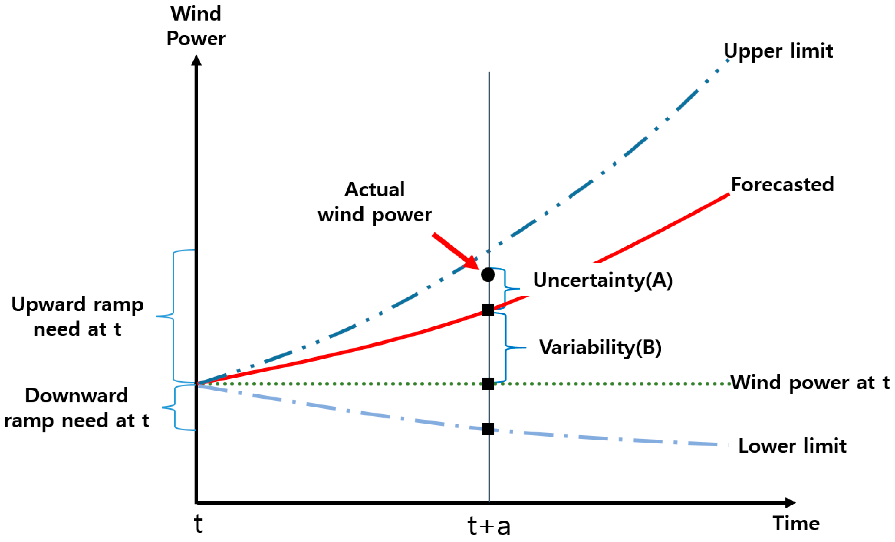
Most methods reported in the literature either use the terms “uncertainty” and “variability” interchangeably or only focus on uncertainty in the forecast data. However, the effects of variability and uncertainty on a system differ. Therefore, the corresponding measures taken by the system operator (SO) to account for them should also differ. The uncertainty is represented by (A) in Figure 2, and can be expressed as the difference between the forecast wind power and the actual wind power output. It is very difficult to predict by how much the actual wind power output will deviate from the forecast wind power output [21]. Therefore, the uncertainty caused by the forecast error requires operating reserve in order to control the balance between generation and load [14]. The variability is shown by (B) in Figure 2, which is defined as the difference between wind power at time t and wind power output at time (t + a) [2]. This may result in power imbalance due to insufficient ramping capability. As the penetration of renewable energy resources increases, these problems become more severe, and it is therefore becoming increasingly important to determine the appropriate ramping capacity for a system in order to provide flexibility. Here, we propose the FRC method, which considers both uncertainty and variability.

2.2. Modeling System Uncertainties

2.2.1. Load Forecast Error and Conventional Generator Outage

The uncertainty in the forecast load can be described using a Gaussian distribution with a zero mean and a fixed standard deviation [22]. The main source of uncertainties with conventional generation is forced outages of the generation units. The most widely used probability tool is the capacity outage probability table (COPT), which contains all possible power outputs of the committed conventional generation fleet, and a corresponding discrete probability distribution is calculated based on the individual forced outage probabilities of each of the generation units [22].

2.2.2. Wind Power Forecast Error

The uncertainty in the forecast wind power was described using a probability distribution. Models of wind power forecast error typically employ a normal distribution; however, measured data for wind power show that a Gaussian distribution does not well describe the tails in the error distribution in the forecast data [1]. 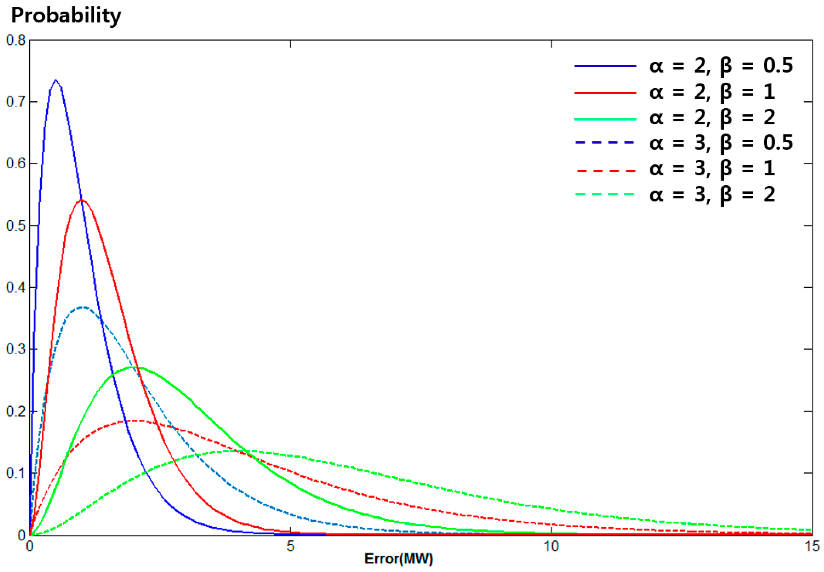Furthermore, wind power generation is asymmetric in terms of the forecast error distribution, and also follows different distributions depending on the generation level [7]. Because of this, to capture the statistics of the error, here the wind power forecast errors were classified into five groups according to wind power level for a given lead time. The low predicted wind powers produce negative forecasts, and when the wind power is high, the forecast errors tend to be positive. Positive error indicates overestimation and negative error indicates underestimation. The probability distribution can be represented using gamma-like densities [7]:

$$\begin{gathered} f_{\mathsf{\gamma }}\left(y\right)=\frac{1}{{\mathsf{\beta }}^{\mathsf{\alpha }}\mathrm{\Gamma }\left(\mathsf{\alpha }\right)}{y}^{\mathsf{\alpha }-1e^{-\frac{y}{\mathsf{\beta }}}};\left\{\mathsf{\alpha },\mathsf{\beta },y\right\}>0 \\ \mathsf{\mu }\triangleq \mathsf{\alpha }\mathsf{\beta };\mathsf{\sigma }\triangleq \sqrt{{\mathsf{\alpha }\mathsf{\beta }}^2} \end{gathered}$$

(1)

where {μ, σ} are functions of the parameters {α, β}, and indicate the mean and standard deviation of the gamma density. Figure 3 shows gamma-like density functions with various α and β where α is a shape parameter, and β is a scale parameter. For simplicity, all wind turbines were assumed to be identical; therefore, the output of a wind farm is N times the output of a single wind turbine.

2.3. Flexible Ramping Capacity

2.3.1. Operating Reserve Constraints

As discussed above, procuring more regulation service to manage wind power variability and forecast uncertainties is inefficient (from the perspective of market efficiency). Accordingly, some power markets, including MISO and CAISO, have proposed creating a new market termed “ramping product”. This is the amount of power output that an on-line generator can increase or decrease within a predetermined time interval. To ensure reliable operation, there must be sufficient ramping capacity to handle a change in net load. However, existing approaches do not consider constraints caused by the operating reserve when evaluating the ramping capability of a generator. This may lead to overestimates of the ramping capacity of resources with AS responsibilities. If a resource being dispatched has AS responsibility at time t, the ramping capability of resources must be reduced to provide some ramping capacity for AS. 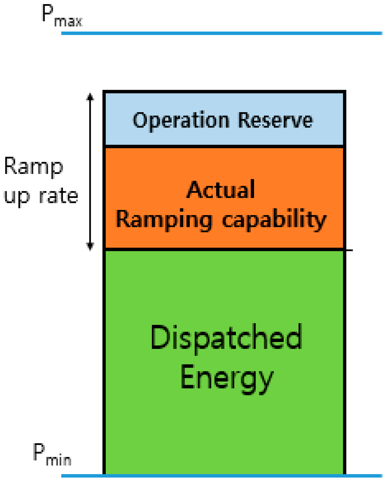Figure 4 illustrates the practical ramping capability of resources, considering operating reserve constraints. The technical upward ramp rate of a generator ranges from the dispatch level to the top of the box. However, since the region shown in blue is retained due to AS awards, the practical ramping capability that the generator can provide becomes limited to the region shown in orange. If this constraint is not considered, it can lead to scarcity events caused by resources that have sufficient power capacity, but insufficient ramping capability [14].

2.3.2. Flexible Ramping Capability Requirement

The target system upward and downward ramping capacity requirements (SURC and SUDC, respectively) can be expressed as follows [14]:

$$\begin{gathered} SUR{C}_t=\max \left[\left(NetDeman{d}_{t+n}-NetDeman{d}_t\right)+Uncertaint{y}_{u{p}_{t+n}},0\right] \\ SDR{C}_t=\max \left[\left(NetDeman{d}_t-NetDeman{d}_{t+n}\right)+Uncertaint{y}_{d{n}_{t+n}},0\right] \end{gathered}$$

(2)

The first terms on the right-hand side of these expressions represent the variability between consecutive time intervals. The second terms are fixed values that correspond to the uncertainty in the net load. With significant variability and uncertainty in a power system, this method cannot prevent power imbalance and price spikes. Here, to improve system reliability and cost efficiency, the amount of FRC required at time t is calculated stochastically:

$$\begin{gathered} SUR{C}_t=\max \left[\left(NetDeman{d}_{t+n}-NetDeman{d}_t\right)+\max (Uncertaint{y}_{u{p}_{t+n}}-Reserv{e}_{t+n},0\right),0] \\ SDR{C}_t=\max \left[\left(NetDeman{d}_t-NetDeman{d}_{t+n}\right)+\max \left(Uncertaint{y}_{d{n}_{t+n}}-Reserv{e}_{t+n},0\right),0\right] \end{gathered}$$

(3)

In general, when the variability of the system net load is positive, (i.e., the net load is increasing), upward ramping capacity is required. Conversely, when the variability is negative, downward ramping capacity is required. When considering the uncertainties in the net load, however, there may be times when both upward and downward ramping capacity is required simultaneously. With FRC method, both upward and downward ramping capacity can be secured, which can satisfy system reliability criteria. The first term in (3) is the ramping capacity for managing the net load variability, and the second term is ramping capacity required to maintain system reliability. The ramping capacity required for uncertainty is calculated as the difference between the upper limit of the net load and the forecast net load at time (t + n). If the operating reserve is insufficient to compensate for this uncertainty, additional capacity is secured via flexible ramping capacity using a stochastic method. The requirements calculated using the FRC method can maintain system reliability above the threshold in all cases, and can reduce the rate of occurrence of price spikes by increasing the system flexibility.

To calculate the additional flexible ramping capacity requirements, the generation margin probability distribution function M was used, which is defined as the difference between the total generation and load. Assuming independence, the system generation margin can be computed using convolution [23]. First, the sum G of the conventional generator output C and the wind generation output W is computed using convolution:

$$P_G\left(G=g\right)={\displaystyle \sum }_{c=-\infty }^{\infty }{P}_W\left(W=g-c\right)P_C\left(C=c\right)$$

(4)

Next, the system generation margin M can be calculated by the convolving the system generation output and load:

$$P_M\left(G-L=m\right)={\displaystyle \sum }_{l=-\infty }^{\infty }{P}_G\left(G=g-l\right)P_L\left(L=l\right)$$

(5)

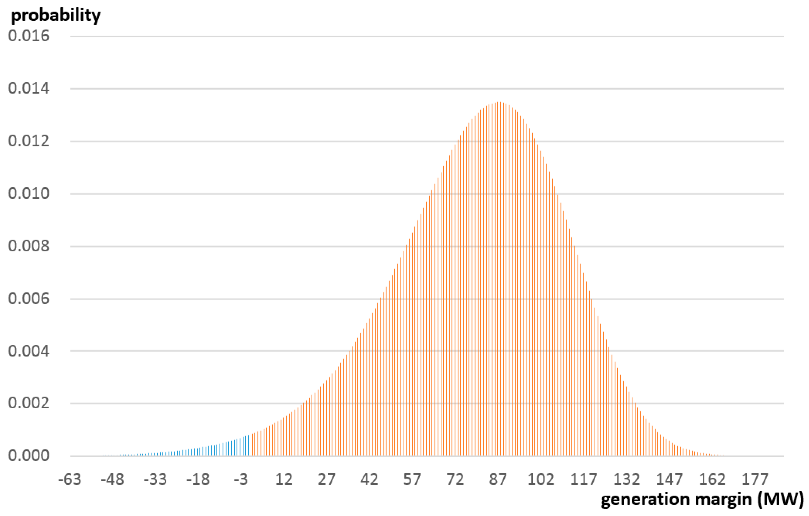
The variable, L, is the load. The system generation margin is the margin by which the available generating capacity exceeds the system net load, and can be expressed using a discrete probability distribution for each look-ahead time, as shown in Figure 5 [4]. The y-axis means probability corresponding to the generation margin. The sum of probabilities of negative generation margin is the loss of load probability (LOLP), which is widely used in power systems analysis. It is calculated by summing the probability that the demand exceeds the available generation capacity [14]. The FRC requirement (see Section 2.3.2) is determined to maintain the LOLP below the threshold for the reliability criteria. Using a stochastic method, we can maintain the system reliability within the reliability threshold and reduce the number of short-term scarcity events due to shortages of ramping capacity.

2.4. Calculation of the Demand Curve

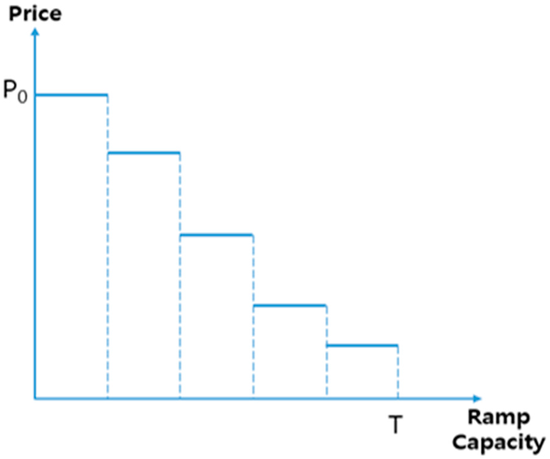
In this section, we define the demand curve for FRC. This indicates the price of the ramping capacity of the system and sets an effective cap on the required ramping capacity that must be procured. Hourly FRC demand curves can be determined based on the FRC requirement. The price of flexible ramping capacity R is represented as follows.

$$P\left(R\right)={\displaystyle \sum }_{m}LOLP\left(R,m\right)\times m\times VOLL-{\displaystyle \sum }_{m}LOLP\left(T,m\right)\times m\times VOLL$$

(6)

Figure 6 shows the FRC demand curve, which is developed every time interval. X-axis of the FRC demand curve represents ramping capacity. Y-axis refers to the price of ramping capacity. T is the maximum FRC that a SO is willing to procure in order to satisfy the system reliability. When the SO has procured FRC with T amount, the system reliability satisfies the given reliability standard, which means the SO does not have to purchase FRC any more even if the FRC price is zero. P refers to the difference between the EENS cost of the case when the SO has procured FRC with T amount and that of the case when the SO has procured with R amount as shown in (6). If the price of FRC is greater than P₀, the cost for purchasing FRC becomes bigger than the EENS cost of the system. Consequently, the SO will take the risk of power imbalance instead of purchasing FRC. In this way, FRC demand curve evaluates the value of the FRC depending on the system condition, and provides a price signal considering system reliability. The SO can achieve reasonable decision making taking account of the tradeoff between system reliability and FRC cost through the FRC demand curve.

3. Mathematical Formulation

The following objective function minimizes the production cost over all scheduling intervals subject to the constraints in (8)–(24):

$$\min {{\displaystyle \sum }}_{t=1}^T{{\displaystyle \sum }}_i^I[C_{i,t}^E\left(v_i\left(t\right),P_i\left(t\right)\right)+C_{i,t}^R(v_i\left(t\right),R_i\left(t\right))]$$

(7)

Here, we sum two components: the energy cost $(C_{i,t}^E)$ and the reserve cost $(C_{i,t}^R)$. The energy cost consists of startup and fuel costs for satisfying the generation-demand balance. The reserve provision cost is imposed on conventional generator. Reserve costs are typically much lower than energy costs. We assume that the operating reserve costs are 20% of the energy marginal cost. The real-time economic dispatch (RTED) model is nonlinear and contains modified constraints. RTED also uses the commitment schedule from the day-ahead UC (DAUC), and optimizes it in RT over a single shorter interval (i.e., 1 h) using actual load and wind power data.

3.1. Generation Limits and Ramping Constraints

The inequalities below describe a power output constraint for each generator and a ramping rate constraint. The generation of each unit must be within the following limits [24]:

$$P_{{\min }_i}\times v_i\left(t\right)\le P_i\left(t\right)\le P_{{\max }_i}\times v_i\left(\mathrm{t}\right)$$

(8)

where the variable P_i(t) is constrained by the ramping constraints:

$$-Ram{p}_{dn,i}\times ResponseTime\le P_i\left(t\right)-P_i\left(t-1\right)\le Ram{p}_{up,i}\times ResponseTime$$

(9)

where, v_i is the commitment variable of unit i, where v_i = 1 if unit i is scheduled to be on during period t, and v_i = 0 otherwise. P_maxi and P_mini are the maximum and minimum output powers of unit i, respectively (MW). Equation (9) represents the ramping constraints of generator i.

3.2. Minimum Up and Down Time Constraints

The expressions describing the minimum up and down time constraints in DAUC are formulated as mixed-integer linear expressions [25]. The minimum up time constraints are as follows.

$${\displaystyle \sum }_{t=1}^{S_i}\left[1-v_i\left(t\right)\right]=0;\forall i\in I$$

(10)

$${\displaystyle \sum }_{n=t}^{t+U{T}_i-1}{v}_i\left(n\right)\ge U{T}_i[v_i\left(t\right)-v_i\left(t-1\right)]$$

(11)

$${\displaystyle \sum }_{n=t}^{24}\{v_i\left(n\right)-\left[v_i\left(t\right)-v_i\left(t-1\right)\right]\}\ge 0;\forall t=24-U{T}_i+2,\dots \dots ,24$$

(12)

The minimum down time constraints are represented as follows:

$${\displaystyle \sum }_{t=1}^{L_i}\left[v_i\left(t\right)\right]=0;\forall i\in I$$

(13)

$${\displaystyle \sum }_{n=t}^{t+D{T}_i-1}\left[1-v_i\left(n\right)\right]\ge D{T}_i[v_i\left(t\right)-v_i\left(t-1\right)]$$

(14)

$${\displaystyle \sum }_{n=t}^{24}\{1-v_i\left(n\right)-\left[v_i\left(t-1\right)-v_i\left(t\right)\right]\}\ge 0;\forall t=24-D{T}_i+2,\dots \dots ,24$$

(15)

where, S_i is the number of periods that unit i must be on-line initially because of its minimum up time constraint h. L_i is the number of periods that unit i must be initially off-line because of its minimum down time constraint h, and UT_i is the minimum up time of unit i.

3.3. Power Balance Constraints

The total generation of all scheduled units during period t must be equal to system net demand:

$${\displaystyle \sum }_{geni}{P}_i\left(t\right)=D\left(t\right)$$

(16)

where, D(t) is the system net demand during period t.

3.4. Operating Reserve Constraints

For system reliability, some operating reserve must be maintained (we assume 5% of the net demand). A generator that is being called upon to provide operating reserve should operate within its upper generation limits [24]:

$${\displaystyle \sum }_{onlinegeni}{P}_{ma{x}_i}\ge D\left(t\right)+OR\left(t\right)$$

(17)

$$P_i\left(t\right)+O{R}_i\left(t\right)\le P_{ma{x}_i}\times v_i\left(t\right)$$

(18)

where, OR(t) is the system operating reserve and OR_i(t) is the operating reserve contribution of unit i during period t (MW).

3.5. Flexible Ramping Capacity Constraints

The following constraints ensure that the total amount of upward and downward flexible ramping capacity can meet the system requirements [15]:

$${\displaystyle \sum }_{onlinegeni}FR{C}_{up,i}\left(t\right)\ge SURC\left(t\right)$$

(19)

$${\displaystyle \sum }_{onlinegeni}FR{C}_{dn,i}\left(t\right)\ge SDRC\left(t\right)$$

(20)

where, FRC_up,i(t) and FRC_dn,i(t) are the upward and downward flexible ramping capacities of unit i during period t, and SURC(t) and SDRC(t) are the system upward and downward ramping capacity requirements during period t, respectively.

The upward and downward FRC during each time period t is bounded by the available unloaded resource capacity:

$$P_i\left(t\right)+O{R}_i\left(t\right)+FR{C}_{up,i}\left(t\right)\le P_{ma{x}_i}\times v_i\left(t\right)$$

(21)

$$P_i\left(t\right)-FR{C}_{dn,i}\left(t\right)\ge P_{mi{n}_i}\times v_i\left(t\right)$$

(22)

The Constraints (21) and (22) describe minimum and maximum power constraints of each generator considering the FRC. Constraint (21) limits the sum of the awards of energy schedule, operating reserve and upward flexible ramping capacity to be less than or equal to the unit’s maximum power. Constraint (22) ensures minimum power limit. The deployment of procured downward flexible ramping capacity should not violate unit’s minimum power constraint.

In this paper, we do not consider the downward operating reserves.

$$FR{C}_{up,i}\left(t\right)+O{R}_i\left(t\right)\le Ram{p}_{up,i}\times ResponseTime\times v_i\left(t\right)$$

(23)

$$FR{C}_{dn,i}\left(t\right)\le Ram{p}_{dn,i}\times ResponseTime\times v_i\left(t\right)$$

(24)

In Equation (23), the sum of the ramping capabilities plus the upward reserves provided by a unit should be limited to the ramp rate of the resource. The response time is the time after which the operating reserve and ramping capacity provided by generator i is deployable. The day-ahead interval is 1 h, and the real-time interval is 5 min. This constraint ensures that the generators in the system can provide the required ramping capability.

3.6. System Reliability Threshold Constraints

The hourly system reliability (LOLP) should always satisfy the reliability threshold ($\propto$). The hourly FRC requirement will be adjusted to maintain the reliability level.

$$LOL{P}_t\left(t\right)\le \propto \left(Reliabilitythreshold\right).$$

(25)

4. Simulation and Discussion

We carried out simulations to explore the benefits of the proposed FRC method and analyze its impact on generation scheduling of DAUC and RTED. The DAUC produces optimal generation scheduling, including commitment status, reserve schedule, and ramping capacity over 24 h. The RTED model takes the DAUC results as inputs, and produces the least-cost dispatch schedules at 5-min intervals for 1 h. We developed FRC demand curves, which indicate the value of the ramping capacity of the system.

This section is divided into two parts. The first compares generation schedules and expected operating cost between the conventional method and the proposed FRC method. The expected operating cost is computed as the sum of the production costs and expected energy not served (EENS) costs, assuming that the value of lost load (VOLL) is $1000/MWh. EENS cost models describe the economic losses imposed on the demand side in case of interruptions of electrical power [26]. The second part of this section illustrates how the FRC model affects the system reliability and expected operating costs, and how this depends on the level of wind power generation.

The test system was a modified 10-unit system consisting of thermal units and wind power plants, where the output was described as a negative load [27]. Wind turbines were considered to be non-schedulable, and could supply the power up to the maximum available wind power. We do not consider transmission constraints for simplicity, and focus on the impact of the FRC model.

Table 1. Generator data for the 10-unit system [27].

Unit No.	1	2	3	4	5	6	7	8	9	10
Cost coefficient
a ($/h)	1000	970	700	680	450	370	480	660	665	670
b ($/MWh)	16.19	17.26	16.6	16.5	19.7	22.26	27.74	25.92	27.27	27.79
c ($/MW2h)	0.00048	0.00031	0.002	0.00211	0.00398	0.00712	0.00079	0.00413	0.00222	0.00173
Pmax (MW)	455	455	130	130	162	80	85	55	55	55
Pmin (MW)	150	150	20	20	25	20	25	10	10	10
Min up (h)	8	8	5	5	6	3	3	1	1	1
Min down (h)	8	8	5	5	6	3	3	1	1	1
Start-up cost ($)	4500	5000	550	560	900	170	260	30	30	30
Initial state (h)	8	8	−5	−5	−6	−3	−3	−1	−1	−1
Ramp (MW/h)	150	150	25	25	30	30	30	50	50	50

lists the data on the generators, and

Table 2. Forecast hourly load and wind generation. These data were obtained from the EirGrid website [28].

H	Load (MW)	Wind (MW)	H	Load (MW)	Wind (MW)	H	Load (MW)	Wind (MW)
1	700	351	9	1300	220	17	1000	171
2	750	330	10	1400	158	18	1100	160
3	850	298	11	1450	115	19	1200	181
4	950	315	12	1500	102	20	1400	219
5	1000	316	13	1400	116	21	1300	240
6	1100	285	14	1300	148	22	1100	271
7	1150	277	15	1200	153	23	900	309
8	1200	238	16	1050	187	24	800	320

lists the forecast hourly load and available wind power. The system peak load was 1500 MW, and occurred at hour 12.

4.1. Comparison between the Conventional and Proposed Methods

The following three cases were studied to investigate the impact of the proposed method on optimal DAUC and RTED. The operating reserve was assumed to be 5% of each hourly load, and the total power supplied from wind was set to 21.5% of the daily forecast system load.

• Case 1: Ramping capacity method without operating reserve constraints and flexible ramping capacity requirement.
• Case 2: Ramping capacity method with operating reserve constraints.
• Case 3: Flexible ramping capacity method with operating reserve constraints and flexible ramping capacity requirement.

Case 1 is a conventional ramping model, which does not consider operating reserve constraints. In this model, the ramping capacity to deal with uncertainty in the net load was fixed. Case 2 considers operating reserve constraints, which reflect the available practical ramping capacity of the generation resources. Case 3 is the proposed method with operating reserve constraints and FRC requirement, where the FRC requirement was calculated stochastically depending on the uncertainty in the net load. The system reliability (LOLP) threshold was set to 1% [29].

4.1.1. Results of Day-Ahead Unit Commitment

The changes in the DAUC schedules of generators 3 and 4 were analyzed, and the results are listed in

Table 3. Unit commitment schedules.

Unit		Commitment Schedule (1–24 h)
3	Case 1	000000 011111 111000 000000
	Case 2	000000 111111 111100 000000
	Case 3	000000 111111 111100 000000
4	Case 1	000000 111111 111111 111111
	Case 2	000001 111111 111111 111111
	Case 3	000000 111111 111111 111111

(see the underlined data). With cases 2 and 3, generator #3 was committed during hour 7 and 16. With case 2, generator #4 was committed only during hour 6, while the commitment schedules of the other generators were the same in all cases. Although the target system ramping capacity was the same for cases 1 and 2, the commitment schedules varied. This is because of changes in the available practical ramping capacity of each generator, which reflect the operating reserve constraints.

Comparing cases 2 and 3, the hourly unit commitment also changed. This is because with case 3 the model procured more FRC to maintain system reliability to cover the uncertainty in the net load (see

Table 4. Upward and downward system RC requirements.

Up-Ramp	1	2	3	4	5	6	7	8	9	10	11	17	18	19
Cases 1 & 2	71	132	83	49	131	58	89	118	162	93	63	111	79	162
Case 3	86	166	112	75	152	77	89	118	162	93	63	111	79	162
Down-Ramp	7	11	12	13	14	15	16	18	20	21	22	23
Cases 1 & 2	0	0	114	132	105	184	34	0	121	231	238	111
Case 3	5	11	187	205	178	278	128	15	159	269	276	145

). Conventional methods only consider either upward or downward ramping capacity, depending on whether the change in the net load is negative or positive. However, the proposed method considers the ramping requirements in both directions.

As listed in

Table 5. Expected operating costs with DAUC.

Case	Production Cost ($)	EENS Cost ($)	Operating Cost ($)
Case 1	464,155.82	32,775.61	496,931.43
Case 2	465,381.49 (+0.26%)	2,720.05 (−91.7%)	468,101.53 (−5.8%)
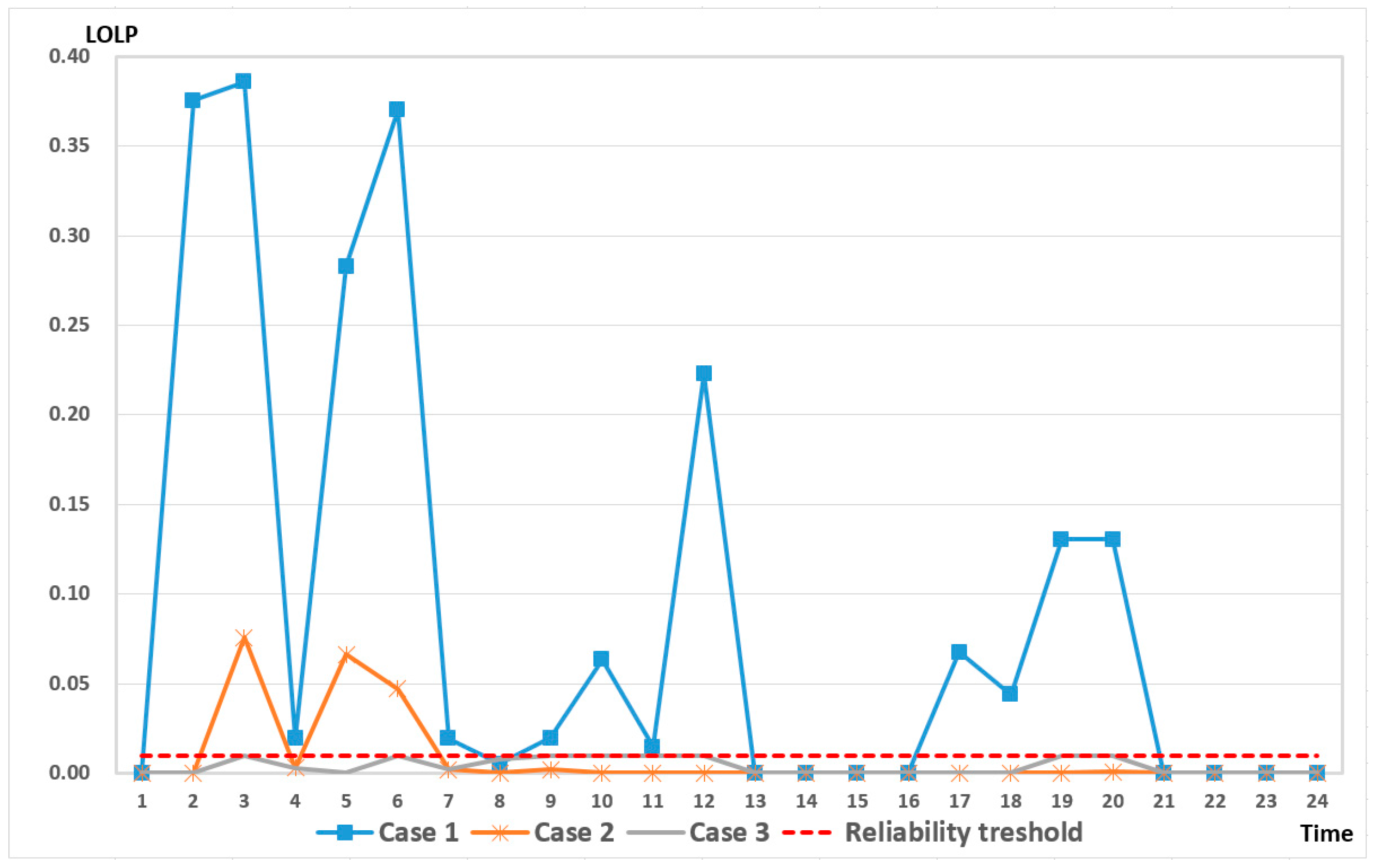
Case 3	465,294.29 (+0.25%)	337.57 (−98.9%)	465,631.86 (−6.3%)

, the production costs of case 2 increased by 0.26% compared with those of case 1. This is because more expensive resources were committed. However, the total expected operating cost was 5.8% lower with case 2 than with case 1. This is because the EENS cost decreased significantly (by 91.7%). Case 1 did not take into account the reduction in the ramping rate of generators with a reserve obligation. Therefore, if net load were to increase, LOLP would increase significantly due to the lack of available ramping capacity, as shown in Figure 7. With case 3, there were significant savings in terms of the EENS cost because LOLP was maintained below a certain level by ensuring greater system flexibility. The simulation results show that the proposed FRC method was the most economic.

Figure 7 shows the hourly LOLP for each case. With cases 1 and 2, the LOLP exceeded the reliability threshold. However, with case 3, the LOLP remained below the reliability threshold during all time periods. The conventional method did not consider the operating reserve constraints, which led to a significant increase in the LOLP because of a lack of capacity to handle large variations in net load. In other words, if practical ramping capability is not taken into account, system flexibility may be overestimated. However, using the proposed FRC method, system reliability was enhanced significantly. Thus, these simulations show that the FRC method is effective in terms of both supply reliability and economics. This is achieved by avoiding the dispatch of additional reserve resources to maintain system reliability, and thus avoiding the associated short-term price spikes.

The downward ramping capacity did not influence the commitment schedule in these simulations. This is because the downward ramping capability of an online generator was sufficient to cope with the uncertainty and variability of the net load. If load decreases significantly at the same time as wind power generation greatly increases, situations in which downward ramping capacity may be insufficient are more likely to occur.

4.1.2. Results of Real-Time Economic Dispatch

RTED was carried out based on the commitment output from the DAUC model at hour 20.

Table 6. Real-time economic dispatch schedules at hour 20.

Unit		0	5	10	15	20	25	30	35	40	45	50	55
1	Case 1	453	448	453	451	453	443	453	453	445	453	453	449
	Case 2	449	441	453	447	451	439	451	453	448	453	453	450
	Case 3	445	437	448	441	451	439	451	450	445	450	453	447
5	Case 1	141	143	146	148	151	148	148	148	145	147	149	147
	Case 2	145	146	147	148	150	147	148	148	145	147	148	145
	Case 3	148	149	152	153	153	150	151	151	152	153	151	148

lists the results of generation scheduling of units #1 and #5 for each case. Unit #1 was the least expensive base-load unit, and unit #5 was the marginal unit at hour 20. With case 2, the ramping capacity of resources with AS responsibility was reduced compared with that of case 1 because of operating reserve constraints. To compensate for the shortage of ramping capacity, the power output of unit #1 was reduced to provide the ramping capacity. The power output of unit #5 increased because of the reduction in the power output of unit #1, which resulted in an increase in the production cost. With case 3, which considered the system uncertainty and the required additional FRC, the changes in output powers of units #1 and #5 were more significant.

The proposed FRC method resulted in greater system flexibility (see

Table 7. System RC requirements for ED.

Up-Ramp	5	10	15	25	30	35	40	45	50
Cases 1 & 2	21	0	17	23	0	0	9	4	0
Case 3	27	2	23	27	11	1	20	15	3
Down-Ramp	0	15	25	35	40	45	50	55
Cases 1 & 2	14	9	31	0	10	0	0	8
Case 3	26	21	31	12	22	3	8	20

). The increased ramping capacity requirement in case 3 contributed to the reduced EENS cost (see

Table 8. The expected operating costs with RTED.

Case	Production Cost ($)	EENS Cost ($)	Operating Cost ($)
Case 1	25,103.02	1,475.72	26,578.74
Case 2	25,111.44 (+0.03%)	126.55 (−91.4%)	25,237.99 (−5.04%)
Case 3	25,124.78 (+0.08%)	100.38 (−93.2%)	25,225.16 (−5.09%)

). This in turn resulted in a reduction in the expected operation costs and maintained system reliability, as shown in Figure 8. In short, the conventional method resulted in situations where ramping capacity was insufficient to satisfy the change in the net load. To maintain system reliability, the operating reserve should be more ensured, which will lead to a significant increase in the production cost.

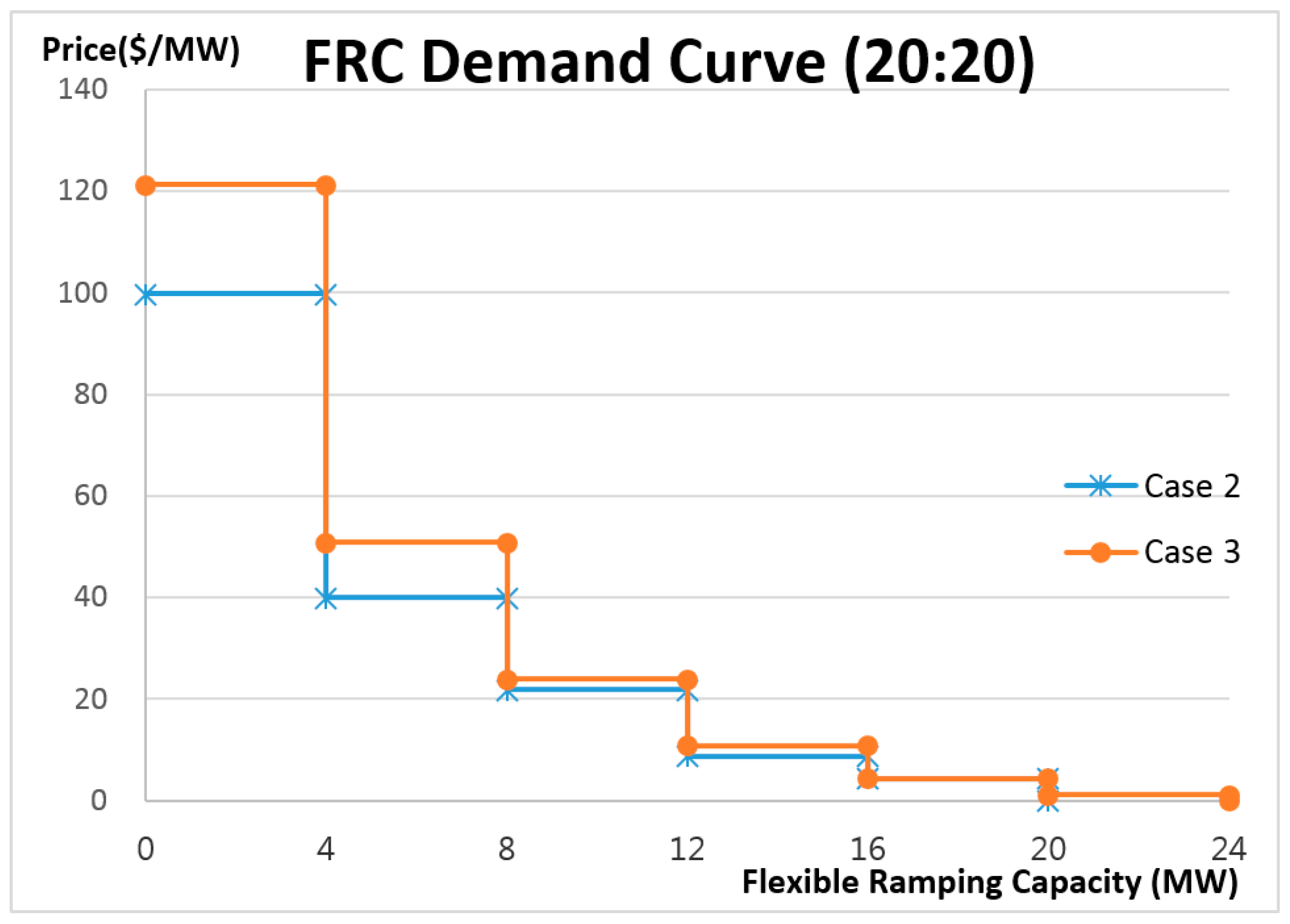
The FRC demand curves at a specific time (20:20) for RTED with cases 2 and 3 are shown in Figure 9. The required quantity of FRC was higher with case 3 because we must secure more ramping capacity to satisfy the reliability criteria (LOLP < 0.01); this led to a significant decrease in the EENS costs compared with those in cases 1 and 2. Therefore, price levels of the corresponding ramping capacity were higher with case 3. Although the conventional methods did not reflect the practical value of ramping capacity, the proposed FRC method could describe the practical economic value of ramping capacity considering system reliability.

4.2. Impact of the Wind Energy Level

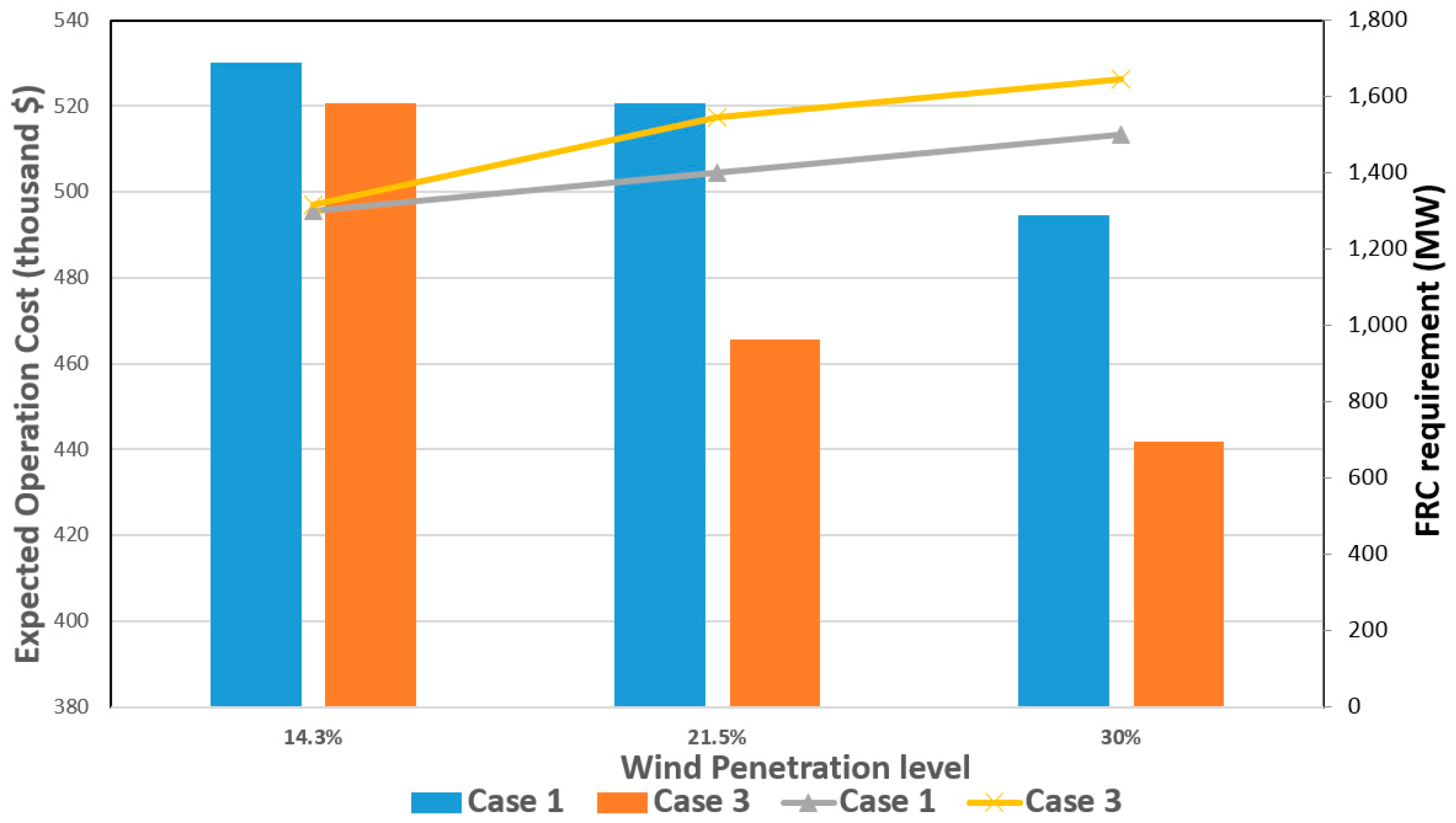
In this section, we discuss the impact of the level of wind power generation. Cases with wind generation of daily load forecasts of 14.3%, 21.5%, and 30% were investigated using simulations. Figure 10 shows the expected operating costs and FRC requirements as a function of the level of wind power generation with cases 1 and 3. For all cases, as the wind power increased, the expected operating cost decreased due to a decrease in the generation of (relatively expensive) conventional units. The reduction in cost was more significant with case 3 because the FRC method considers the hourly system reliability. Moreover, the hourly ramping capacity requirement increased as the wind power generation level increased, which in turn resulted in increases in system uncertainty and variability.

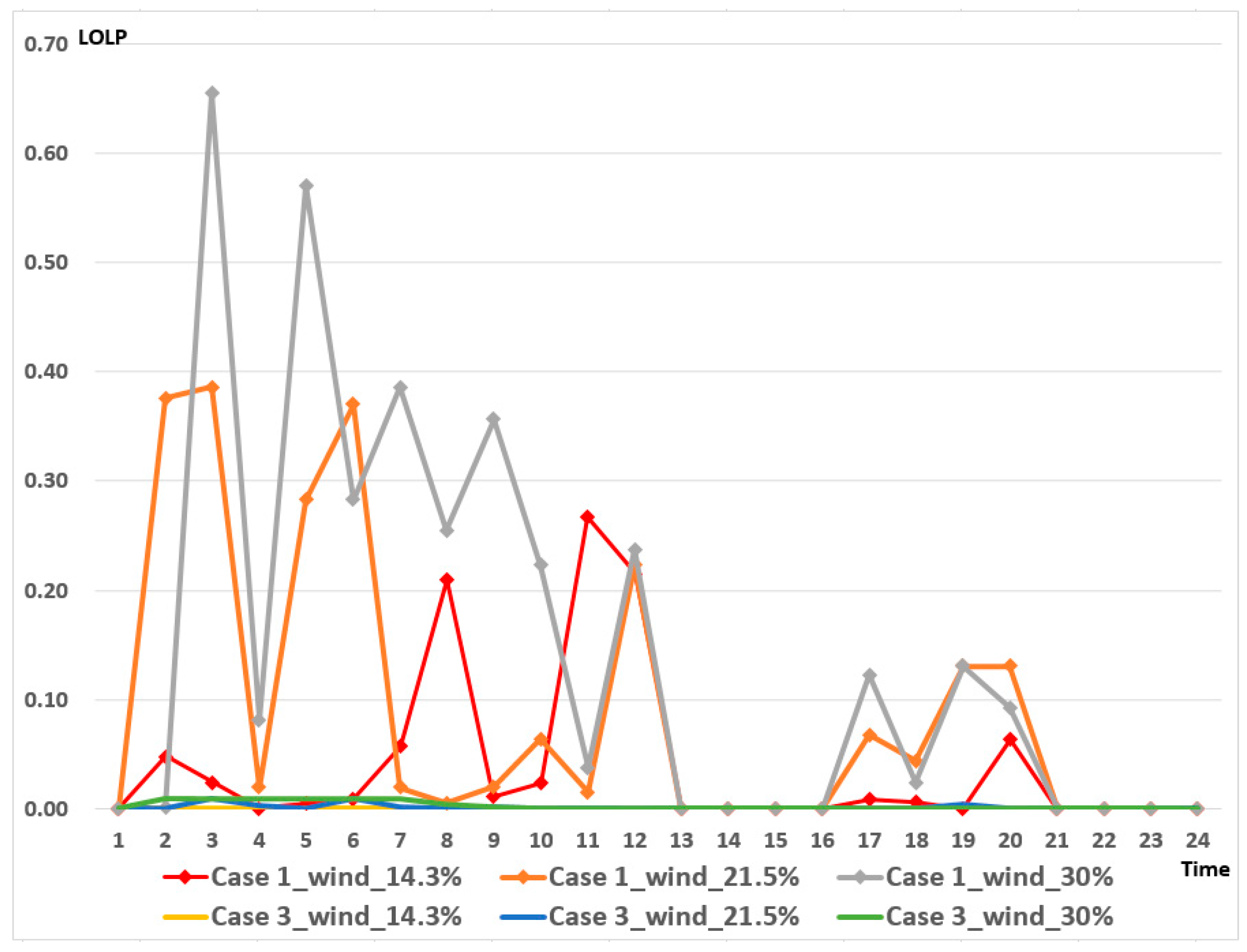
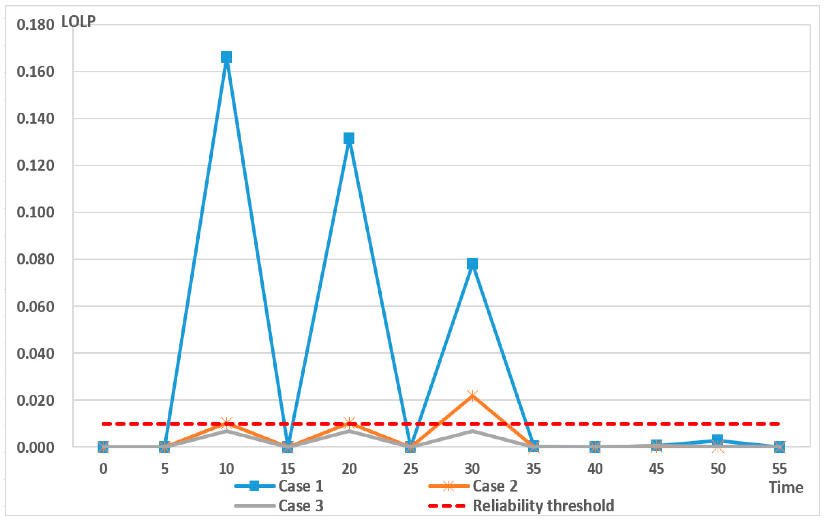
Figure 11 shows the system reliability at different wind power generation levels. With case 1, as the wind power generation increased, the LOLP also increased, as did the number of events whereby the LOLP exceeded the reliability criteria. By contrast, with case 3, we can clearly see that the system reliability was maintained regardless of the wind power generation level. Consequently, these results show that the proposed FRC method could accommodate wind power generation with improved economic efficiency while satisfying the system reliability criteria.

5. Conclusions

We have described a model for generation scheduling with FRC. This model takes into account uncertainties in the net load and operating reserve constraints. A stochastic approach was used to account for uncertainty and variability of net load, and operating reserve constraints were considered when measuring ramping capacity of generating units with AS responsibility.

The proposed method was shown to exhibit significant reliability improvements, as well as improved economic efficiency by altering commitment and dispatch. Our simulation studies showed that the hourly LOLP could be maintained below the reliability threshold, and the expected operating costs could be reduced. As the wind power generation increased, the reduction in the expected operating cost became greater. The proposed FRC model enabled a reduction in the EENS cost by securing FRC considering the practical ramping capability of the generation resources. The FRC method also allowed us to calculate the FRC demand curve, which quantifies the economic value of the hourly ramping capacity product. The prices of the FRC demand curves reflect hourly system reliability as a function of the FRC. In other words, the FRC demand curve represents the economic value of hourly system reliability. The proposed method also showed improved economic efficiency and system reliability in accommodating increased wind power.

As part of future research, we intend to investigate the impact of generating schedules that consider an FRC model with demand response in both UC and ED processes.

References

- Martinez-Cesena, E.A.; Mutale, J. Impact of wind speed uncertainty and variability on the planning and design of wind power projects in a smart grid environment. In Proceedings of the 2011 2nd IEEE Power and Energy Society (PES) International Conference and Exhibition on Innovative Smart Grid Technologies (ISGT Europe), Manchester, UK, 5–7 December 2011.
- Xu, L.; Tretheway, D. Flexible Ramping Products; California ISO: Folsom, CA, USA, 2012. [Google Scholar]
- Ferreira, C.; Gama, J.; Matias, L.; Botterud, A.; Wang, J. A Survey on Wind Power Ramp Forecasting; No. ANL/DIS-10-13; Argonne National Laboratory (ANL): Lemont, IL, USA, 2011.
- Matos, M.A.; Bessa, R.J. Setting the operating reserve using probabilistic wind power forecasts. IEEE Trans. Power Syst. 2011, 26, 594–603. [Google Scholar] [CrossRef]
- Matos, M.A.; Bessa, R. Operating reserve adequacy evaluation using uncertainties of wind power forecast. In Proceedings of the IEEE PowerTech 2009, Bucharest, Romania, 28 June–2 July 2009.
- Zhi, Z.; Botterud, A. Dynamic Scheduling of Operating Reserves in Co-Optimized Electricity Markets with Wind Power. IEEE Trans. Power Syst. 2014, 29, 160–171. [Google Scholar] [CrossRef]
- Menemenlis, N.; Huneault, M.; Robitaille, A. Computation of Dynamic Operating Balancing Reserve for Wind Power Integration for the Time-Horizon 1–48 h. IEEE Trans. Sustain. Energy 2012, 3, 692–702. [Google Scholar] [CrossRef]
- Papavasiliou, A.; Oren, S.S.; O’Neill, R.P. Reserve requirements for wind power integration: A scenario-based stochastic programming framework. IEEE Trans. Power Syst. 2011, 26, 2197–2206. [Google Scholar] [CrossRef]
- Streiffert, D.; Philbrick, R.; Ott, A. A mixed integer programming solution for market clearing and reliability analysis. In Proceedings of the 2005 IEEE PES General Meeting, San Francisco, CA, USA, 2–16 June 2005.
- Sioshansi, R.; Short, W. Evaluating the impacts of real-time pricing on the usage of wind generation. IEEE Trans. Power Syst. 2009, 24, 516–524. [Google Scholar] [CrossRef]
- Mount, T.; Anderson, L.; Cardell, J.; Lamadrid, A.; Maneevitjit, S.; Thomas, B.; Zimmerman, R. The economic implications of adding wind capacity to a bulk power transmission network. In Proceedings of the 21st Annual Western Center for Research in Regulated Industries Conference, Monterey, CA, USA, 18–20 June 2008.
- Morales, J.M.; Conejo, A.J.; Perez-Ruiz, J. Economic Valuation of Reserves in Power Systems with High Penetration of Wind Power. IEEE Trans. Power Syst. 2009, 24, 900–910. [Google Scholar] [CrossRef]
- Hargreaves, J.J.; Hobbs, B.F. Commitment and dispatch with uncertain wind generation by dynamic programming. IEEE Trans. Sustain. Energy 2012, 3, 724–734. [Google Scholar] [CrossRef]
- Navid, N.; Rosenwald, G. Ramp Capability Product Design for MISO Markets. Available online: https://www.misoenergy.org/Library/Repository/Communication%20Material/Key%20Presentations%20and%20Whitepapers/Ramp%20Product%20Conceptual%20Design%20Whitepaper.pdf (accessed on 8 December 2016).
- Navid, N.; Rosenwald, G. Market solutions for managing ramp flexibility with high penetration of renewable resource. IEEE Trans. Sustain. Energy 2012, 3, 784–790. [Google Scholar] [CrossRef]
- Abdul-Rahman, K.H.; Alarian, H.; Rothleder, M.; Ristanovic, P.; Vesovic, B.; Lu, B. Enhanced system reliability using flexible ramp constraint in CAISO market. In Proceedings of the 2012 IEEE PES General Meeting, San Diego, CA, USA, 22–26 July 2012.
- Wang, C.; Luh, P.B.; Navid, N. Requirement design for a reliable and efficient ramp capability product. In Proceedings of the 2013 IEEE PES General Meeting, Vancouver, BC, Canada, 21–25 July 2013.
- Wang, B.; Hobbs, B.F. A flexible ramping product: Can it help real-time dispatch markets approach the stochastic dispatch ideal? Electr. Power Syst. Res. 2014, 109, 128–140. [Google Scholar] [CrossRef]
- Chen, R.; Wang, J.; Botterud, A.; Sun, H. Wind Power Providing Flexible Ramp Product. IEEE Trans. Power Syst. 2016. [Google Scholar] [CrossRef]
- Wu, H.; Shahidehpour, M.; Alabdulwahab, A.; Abusorrah, A. Thermal generation flexibility with ramping costs and hourly demand response in stochastic security-constrained scheduling of variable energy sources. IEEE Trans. Power Syst. 2005, 30, 2955–2964. [Google Scholar] [CrossRef]
- Ela, E.; Malley, M.O. Scheduling and Pricing for Expected Ramp Capability in Real-Time Power Markets. IEEE Trans. Power Syst. 2016, 31, 1681–1691. [Google Scholar] [CrossRef]
- Billinton, R.; Allan, R.N. Reliability Evaluation of Power Systems; Plenum Press: New York, NY, USA, 1984; Volume 2. [Google Scholar]
- Williamson, R.C.; Downs, T. Probabilistic arithmetic. I. Numerical methods for calculating convolutions and dependency bounds. Int. J. Approx. Reason. 1990, 4, 89–158. [Google Scholar] [CrossRef]
- Carrión, M.; Arroyo, J.M. A computationally efficient mixed-integer linear formulation for the thermal unit commitment problem. IEEE Trans. Power Syst. 2006, 21, 1371–1378. [Google Scholar] [CrossRef]
- Aminifar, F.; Fotuhi-Firuzabad, M. Reliability-constrained unit commitment considering interruptible load participation. Iran. J. Electr. Electron. Eng. 2007, 3, 10–20. [Google Scholar]
- Liu, G.; Tomsovic, K. Quantifying spinning reserve in systems with significant wind power penetration. IEEE Trans. Power Syst. 2012, 27, 2385–2393. [Google Scholar] [CrossRef]
- Kazarlis, S.A.; Bakirtzis, A.; Petridis, V. A genetic algorithm solution to the unit commitment problem. IEEE Trans. Power Syst. 1996, 11, 83–92. [Google Scholar] [CrossRef]
- Eirgrid Smart Grid Dashboard. Available online: http://smartgriddashboard.eirgrid.com/ (accessed on 8 December 2016).
- Liu, K.; Zhong, J. Generation dispatch considering wind energy and system reliability. In Proceedings of the 2010 IEEE PES General Meeting, Detroit, MI, USA, 24–28 July 2010.
© 2016 by the authors; licensee MDPI, Basel, Switzerland. This article is an open access article distributed under the terms and conditions of the Creative Commons Attribution (CC-BY) license (http://creativecommons.org/licenses/by/4.0/).