A Parallel Probabilistic Load Flow Method Considering Nodal Correlations

Abstract

With the introduction of more and more random factors in power systems, probabilistic load flow (PLF) has become one of the most important tasks for power system planning and operation. Cumulants-based PLF is an effective algorithm to calculate PLF in an analytical way, however, the correlations among the nodal injections to the system level have rarely been studied. A novel parallel cumulants-based PLF method considering nodal correlations is proposed in this paper, which is able to deal with the correlations among all system nodes, and avoid the Jacobian matrix inversion in the traditional cumulants-based PLF as well. In addition, parallel computing is introduced to improve the efficiency of the numerical calculations. The accuracy of the proposed method is validated by numerical tests on the standard IEEE-14 system, comparing with the results from Correlation Latin hypercube sampling Monte Carlo Simulation (CLMCS) method. And the efficiency and parallel performance is proven by the tests on the modified IEEE-300, C703, N1047 systems with distributed generation (DG). Numerical simulations show that the proposed parallel cumulants-based PLF method considering nodal correlations is able to get more accurate results using less computational time and physical memory, and have higher efficiency and better parallel performance than the traditional one.

1. Introduction

With the introduction of more and more uncertainties, such as load fluctuations, variations of distributed generation (DG) into power systems, there is an increasing need to analyze the power system using probabilistic load flow (PLF) methods. PLF is able to take various kinds of random factors into consideration and obtain the probabilistic descriptions of a power system. This method contributes mainly to power system planning, and it can also provide guidance for power system operation [1].

PLF method was first proposed by Borkowska in 1974 [2], and since then PLF has been widely used and studied. In [3], traditional PLF methods were mainly classified into simulation-based methods [4] and analytical methods [5], and some other schemes were also used to calculate the PLF [6,7]. Simulation-based methods require a huge amount of steady-state load flow calculations to determine the statistical characteristics of those random variables, while analytical methods can work out the probabilistic features of the random variables through one-time calculation. Among the analytical methods, PLF based on cumulants is one of the most widely used ones [8]. The cumulants-based PLF method can use the cumulants to avoid the complex convolution computation in stochastic production simulation of power systems [1], and thus has faster calculation speed. However, traditional cumulants-based PLF methods usually ignore the correlations among nodal power injections. Hernández [9] and Sun et al. [10] analyzed the impact of the correlation among the random variables. Usaola et al. [11] and Shi et al. [12] dealt with the wind power correlation by inverse transformation of uniform distribution and Cholesky decomposition. Fan et al [13] proposed joint cumulants to deal with the photovoltaic generation, and other approaches to deal with correlation such as extended point estimate method [14], Hybrid Latin Hypercube Sampling with Cholesky decomposition [15] were also proposed. Although these schemes are proposed to deal with specific nodal injection correlations [11,12,13,14,15], such as the wind speed correlations between neighboring wind power plants, seldom have any studies taken into account the correlations among all the nodes at a power system level [16]. On the other hand, there is also a big defect in that the cumulants-based PLF method needs large amounts of storage and calculation due to the use of the inverse of the sparse Jacobian matrices, so it cannot be adapted to the memory and speed requirements of modern large-scale electric power system applications. Therefore, this paper focuses on the improvement of the analytical PLF method, and a novel algorithm for cumulants-based PLF is proposed, which can deal with the correlations among all system nodes, and avoid the the Jacobian matrix inversion and full matrix manipulation as well.

Parallel computation originated in the latter half of the 20th century, when the University of Illinois and Burroughs Company developed the first parallel computer ILLIAC-IV [17]. Then parallel computation entered a fast-development period, and many parallel computers, such as the Cray-1, Denelcor HEP, and Sequent, began to appear. Parallel computation for power system power flow calculations [18,19], and power system transient stability analysis [20,21], were consecutively developed also. Traditional PLF based on serial computing would be rather time-consuming because of the numerous simulations needed for all possible occasions, and the matrix inversion and full matrix manipulation, therefore, a novel PLF algorithm based on parallel computing is introduced in this paper.

The structure of this paper is as follows: Section 2 introduces the basic theory of the cumulants-based PLF method. The novel PLF algorithm considering the nodal correlations is presented in Section 3. The parallel computing scheme is developed to further improve the proposed PLF algorithm in Section 4. Section 5 evaluates the accuracy, efficiency and parallel performance of the novel PLF algorithm through various case studies on standard or modified test systems. Finally, Section 6 presents the main conclusions of this paper.

2. Theory of Probabilistic Load Flow

The principle of the cumulants-based PLF consists of the probability theory, probabilistic modeling, and series expansion method for the random variables [1].

2.1. Basics of Probability

For continuous random variable $X$, the cumulative probabilistic distribution can be described by Equation (1):

$$F\left(x\right)=P\left\{X\le x\right\}=P\left\{-\infty <X\le x\right\}={\displaystyle \underset{-\infty }{\overset{x}{\int }}f\left(t\right)\mathrm{d}t}$$

(1)

where $F\left(x\right)$ is the cumulative distribution function of the random variable $X$, $f\left(x\right)$ is probability density function of the random variable $X$.

The expectation $E\left(X\right)$ and variance $D\left(X\right)$ of the random variable $X$ are as follows:

$$E\left(X\right)={\displaystyle \underset{-\infty }{\overset{+\infty }{\int }}xf\left(x\right)}\mathrm{d}x$$

(2)

$$D\left(X\right)=E\left\{{\left[X-E\left(X\right)\right]}^2\right\}$$

(3)

The $k$-th order moment $m_k$ and central moment $M_k$ of the random variable $X$ can be calculated through its probability density function and expectation:

$$m_k={\displaystyle \underset{-\infty }{\overset{+\infty }{\int }}{x}^{k}f\left(x\right)}\mathrm{d}x$$

(4)

$$M_k={\displaystyle \underset{-\infty }{\overset{+\infty }{\int }}{\left(x-E\left(X\right)\right)}^{k}f\left(x\right)}dx$$

(5)

The cumulants of the random variable X are then defined by Equation (6).

$$\log \mathsf{\phi }\left(t\right)=\log \left(1+{\displaystyle \sum _{s=1}^{\infty }\frac{m_s}{s!}}{\left(it\right)}^s\right)={\displaystyle \sum _{s=1}^{\infty }\frac{k_s}{s!}}{\left(it\right)}^s$$

(6)

where $k_s$ is the cumulant of the random variable $X$, $\mathsf{\phi }\left(t\right)$ is characteristic function of the random variable $X$, and it can be acquired from the cumulative distribution function $F\left(x\right)$ through Equation (7):

$$\mathsf{\phi }\left(t\right)={\displaystyle \underset{-\infty }{\overset{+\infty }{\int }}{\mathrm{e}}^{itx}\mathrm{d}F\left(x\right)}$$

(7)

According to the definition of cumulants, the following properties can be drawn:

(a)

The cumulants meet the additivity condition. If $Y=X_1+X_2$, and $X_1$, $X_2$ are independent of each other, the following expression can be derived:

$$Y^{\left(k\right)}=X_1{}^{\left(k\right)}+X_2{}^{\left(k\right)}$$

(8)

where $Y^{\left(k\right)}$, $X_1{}^{\left(k\right)}$, $X_2{}^{\left(k\right)}$ are separately the $k$-th order culumants of $Y$, $X_1$, $X_2$.

(b)

The cumulants meet the homogeneity condition. If $Y=aX$, the $k$-th order cumulants of $Y$ will be equal to the product of the $k$-th order cumulants of $X$ and $a^k$:

$$Y^{\left(k\right)}=a^k{X}^{\left(k\right)}$$

(9)

According to the definitions of cumulants, moment, and central moment, the corresponding relationship among the three types of probability features can be obtained. The three features can be transformed into each other, which is the basis of the cumulants-based PLF method.

2.2. Probabilistic Modeling of Power System Uncertainties

The linearized load flow equations of the probabilistic model are formulated under polar coordinates in this study. The nodal power equation and branch transmitted power equation can be described as follows, according to [22]:

$$\{\begin{array}{c}{P}_i=V_i{\displaystyle \sum _{j=1}^n{V}_j\left(G_{ij}\cos {\mathsf{\theta }}_{ij}+B_{ij}\sin {\mathsf{\theta }}_{ij}\right)}\\ Q_i=V_i{\displaystyle \sum _{j=1}^n{V}_j\left(G_{ij}\sin {\mathsf{\theta }}_{ij}-B_{ij}\cos {\mathsf{\theta }}_{ij}\right)}\end{array}$$

(10)

$$\{\begin{array}{l}{P}_{ij}=-V_i{V}_j\left(G_{ij}\cos {\mathsf{\theta }}_{ij}+B_{ij}\sin {\mathsf{\theta }}_{ij}\right)+t_{ij}{G}_{ij}{V}_i{}^2\hfill \\ Q_{ij}=-V_i{V}_j\left(G_{ij}\sin {\mathsf{\theta }}_{ij}-B_{ij}\cos {\mathsf{\theta }}_{ij}\right)+\left(B_{ij}-b_{ij0}\right)V_i{}^2\hfill \end{array}$$

(11)

where $P_i$ and $Q_i$ are the nodal injected active and reactive power of node $i$, $V_i$ and $V_j$ are the voltage of nodes $i$ and $j$; ${\mathsf{\theta }}_{ij}$ is the angle difference between nodes $i$ and $j$, $G_{ij}$ and $B_{ij}$ are the conductance and susceptance of the branch that connects $i$ and $j$, $t_{ij}$ is the ratio of transformer if applicable; $b_{ij0}$ is half of the line capacitive susceptance.

The steady-state load flow Equations (10) and (11) can be rewritten in a general description of function form as:

$$W=f_1\left(V\right)$$

(12)

$$Z=g\left(V\right)$$

(13)

where $W$, $V$, $Z$ are the vectors for nodal power injection, nodal voltage variables, and the branch transmitted power, respectively.

According to Taylor series expansion, the Equations (12) and (13) can be transformed into linearized equations:

$$\Delta V=J_0{}^{-1}\Delta W=S_0\Delta W$$

(14)

$$\Delta Z=G_0\Delta V=G_0{J}_0{}^{-1}\Delta W=T_0\Delta W$$

(15)

where $\Delta W$, $\Delta V$, $\Delta Z$ are the correction vectors for the nodal power injection, nodal voltage variables, and branch transmitted power, $J_0$ and $G_0$ are the Jacobian matrices of $f_1\left(V\right)$ and $g\left(V\right)$, $S_0$ and $T_0$ are the corresponding sensitivity matrices.

For the probabilistic modeling of DG, different DGs might obey different distributions. For example, the Weibull distribution [23,24] is usually used for the wind speed model as shown in Equation (16), and the probabilistic expression and control strategy for wind power generation can be obtained through Equations (16) and (17):

$$f\left(v\right)=\frac{\mathsf{\alpha }}{\mathsf{\beta }}{\left(\frac{v}{\mathsf{\beta }}\right)}^{\mathsf{\alpha }-1}\exp \left[-{\left(\frac{v}{\mathsf{\beta }}\right)}^{\mathsf{\alpha }}\right]$$

(16)

$$P_{wind}=\{\begin{array}{l}0,v_{wind}\le v_{in},v_{wind}\ge v_{out}\hfill \\ \frac{v_{wind}{}^3-v_{in}{}^3}{v_R{}^3-v_{in}{}^3}{P}_R,v_{in}\le v_{wind}\le v_R\hfill \\ P_R,v_{wind}\ge v_R\hfill \end{array}$$

(17)

where $\mathsf{\alpha }$ and $\mathsf{\beta }$ are the shape and scale parameters of Weibull distribution; $v_{in}$, $v_R$ and $v_{out}$ are the cut-in speed, rated speed, and cut-out speed, respectively.

The Beta distribution [25] is often used to model the fluctuations of solar radiation for photovoltaic power generation, seen in Equation (18). The photovoltaic generation power output can be seen as approximately linearly related to the solar radiation distribution [26]:

$$f\left(r\right)=\frac{\Gamma \left(\mathsf{\alpha }+\mathsf{\beta }\right)}{\Gamma \left(\mathsf{\alpha }\right)\Gamma \left(\mathsf{\beta }\right)}{\left(\frac{r}{r_{\max }}\right)}^{\mathsf{\alpha }-1}{\left(1-\frac{r}{r_{\max }}\right)}^{\mathsf{\beta }-1}$$

(18)

where $r$ and $r_{\max }$ are the actual value and maximum value of the solar radiation separately, $\Gamma$ is the Gamma function for the Beta distribution, which can be expressed as follows:

$$\Gamma \left(x\right)={\displaystyle \underset{0}{\overset{+\infty }{\int }}{\mathrm{e}}^{-t}{t}^{x-1}\mathrm{d}t}$$

(19)

In Equation (18), α and β are the parameters of Beta distribution, which can be calculated through the mean and variance values of the random solar radiation variable $r$:

$$\mathsf{\alpha }=\mathsf{\mu }\left[\frac{\mathsf{\mu }(1-\mathsf{\mu })}{{\mathsf{\sigma }}^2}-1\right]$$

(20)

$$\mathsf{\beta }=\left(1-\mathsf{\mu }\right)\left[\frac{\mathsf{\mu }\left(1-\mathsf{\mu }\right)}{{\mathsf{\sigma }}^2}-1\right]$$

(21)

where $\mathsf{\mu }$ and ${\mathsf{\sigma }}^2$ are the mean and variance of random solar radiation.

The normal distribution is typically chosen to model load variations, which can be shown by Equations (22) and (23):

$$f\left(P_l\right)=\frac{1}{\sqrt{2\mathsf{\pi }}\sqrt{D\left(P_l\right)}}\exp \left(-\frac{{\left(P_l-E\left(P_l\right)\right)}^2}{2D\left(P_l\right)}\right)$$

(22)

$$f\left(Q_l\right)=\frac{1}{\sqrt{2\mathsf{\pi }}\sqrt{D\left(Q_l\right)}}\exp \left(-\frac{{\left(Q_l-E\left(Q_l\right)\right)}^2}{2D\left(Q_l\right)}\right)$$

(23)

where $P_l$ and $Q_l$ are the active and reactive power of load node $l$; $E\left(P_l\right)$, $D\left(P_l\right)$, $E\left(Q_l\right)$, and $D\left(Q_l\right)$ are separately the means and variances of active and reactive power.

2.3. Theory of Traditional Probabilistic Load Flow

According to the property of cumulants in Equation (8), the cumulants of all the power injections at a certain node can be added together no matter they are from a load or DG power source, thusafter the following description can be inferred:

$$\Delta W^{\left(k\right)}=\Delta W_g{}^{\left(k\right)}+\Delta W_l{}^{\left(k\right)}$$

(24)

where $\Delta W^{\left(k\right)}$, $\Delta W_g{}^{\left(k\right)}$ and $\Delta W_l{}^{\left(k\right)}$ are separately the $k$-th order cumulants of the total nodal power injection, the nodal generator injection, and the nodal load power injection.

Considering the correlation of the power injections at the same node, Equation (24) should be modified. Because the correlated power injections of the same node can be added together to form a total power injection given by $\Delta W_{xg}{}^{\left(k\right)}$, and it is independent of the other power injections as $\Delta W_{dl}{}^{\left(k\right)}$ [27], therefore, the Equation (24) can be further transformed into the following equation:

$$\Delta W^{\left(k\right)}=\Delta W_{\mathrm{dl}}{}^{\left(k\right)}+\Delta W_{\mathrm{xg}}{}^{\left(k\right)}$$

(25)

where $\Delta W_{\mathrm{dl}}{}^{\left(k\right)}$, $\Delta W_{\mathrm{xg}}{}^{\left(k\right)}$ are separately the $k$-th order cumulants for the total independent and correlated power injections of the same node.

After obtaining the cumulants for the total nodal power injection, the linearized load flow equations can be used to calculate the cumulants of the nodal voltage variables and branch power in an analytical way. It should be noted that the cumulants may only be considered to the 7-th order for power engineering practice [1], namely that $k=1,2,\dots ,7$ for the following expressions:

$$\Delta V^{\left(k\right)}={\left(S_0\right)}_{•}{}^k\Delta W^{\left(k\right)}(k=1,2,\dots ,7)$$

(26)

$$\Delta Z^{\left(k\right)}={\left(T_0\right)}_{•}{}^k\Delta W^{\left(k\right)}(k=1,2,\dots ,7)$$

(27)

where $\Delta V^{\left(k\right)}$, $\Delta W^{\left(k\right)}$ and $\Delta Z^{\left(k\right)}$ are separately the $k$-th order cumulants for the correction variables of the nodal state variables, the nodal power injection and branch transmitted power; ‘${}_{•}$’ denotes the operator for elementwise product of a matrix (Adama product), for example, ${\left(S_0\right)}_{•}{}^k$ is a matrix with each element equal to the $k$-th power of the element in matrix $S_0$.

The cumulants of each order can be calculated consecutively by the method of stochastic production simulation [1]. According to the linearized load flow equations in (14) and (15), the cumulants and central moments of the nodal state variables and branch transmitted power can be obtained. To transform the cumulants into probabilistic distribution, Gram-Charlier expansion [8], Cornish-Fisher expansion [28] and some other series expansions were presented. Gram-Charlier series expansion is adopted in this paper to transform the cumulants into probability distribution:

$$F\left(x\right)={\displaystyle \underset{\overline{x}}{\overset{\infty }{\int }}{\mathsf{\phi }}_1\left(x\right)}\mathrm{d}x+{\mathsf{\phi }}_1\left(\overline{x}\right)\left[{\displaystyle \sum _{i=2}^6{c}_i{H}_i\left(\overline{x}\right)}\right]$$

(28)

where $c_i$ is the coefficient of series expansion, $H_i\left(\overline{x}\right)$ is the Hermite polynomial [1], ${\mathsf{\phi }}_1\left(x\right)$ is the probability density function of normal distribution, $\overline{x}$ is normalized random variables, which has the following expression:

$$\overline{x}=\frac{x-\mathsf{\mu }}{\mathsf{\sigma }}$$

(29)

where $\mathsf{\mu }$, $\mathsf{\sigma }$ are separately the mean value and standard deviation of the random variables.

2.4. Flowchart of Traditional Probabilistic Load Flow

According to the theory above, the block diagram for the traditional cumulants-based PLF algorithm can be shown as in Figure 1. It can be divided into four steps, and the third and fourth step can be easily implemented with parallel computing, which is explained in the following sections.

3. The Novel Probabilistic Load Flow Algorithm Considering Nodal Correlations

3.1. Correlations between Random Variables

For random variables related to each other, the covariance matrix $\mathrm{Cov}$ and correlation matrix $C$ can be used to quantitatively describe their correlations:

$$\mathrm{Cov}=\left[\begin{array}{llll}\mathrm{cov}\left(X_1,X_1\right)\hfill & \mathrm{cov}\left(X_1,X_2\right)\hfill & \cdots \hfill & \mathrm{cov}\left(X_1,X_n\right)\hfill \\ \mathrm{cov}\left(X_2,X_1\right)\hfill & \mathrm{cov}\left(X_2,X_2\right)\hfill & \cdots \hfill & \mathrm{cov}\left(X_2,X_n\right)\hfill \\ ⋮\hfill & ⋮\hfill & \ddots \hfill & ⋮\hfill \\ \mathrm{cov}\left(X_n,X_1\right)\hfill & \mathrm{cov}\left(X_n,X_2\right)\hfill & \cdots \hfill & \mathrm{cov}\left(X_n,X_n\right)\hfill \end{array}\right]$$

(30)

$$C=\left[\begin{array}{llll}\mathsf{\rho }\left(X_1,X_1\right)\hfill & \mathsf{\rho }\left(X_1,X_2\right)\hfill & \cdots \hfill & \mathsf{\rho }\left(X_1,X_n\right)\hfill \\ \mathsf{\rho }\left(X_2,X_1\right)\hfill & \mathsf{\rho }\left(X_2,X_2\right)\hfill & \cdots \hfill & \mathsf{\rho }\left(X_2,X_n\right)\hfill \\ ⋮\hfill & ⋮\hfill & \ddots \hfill & ⋮\hfill \\ \mathsf{\rho }\left(X_n,X_1\right)\hfill & \mathsf{\rho }\left(X_1,X_2\right)\hfill & \cdots \hfill & \mathsf{\rho }\left(X_n,X_n\right)\hfill \end{array}\right]$$

(31)

where the covariance $\mathrm{cov}\left(X_i,X_j\right)$ and correlation $\mathsf{\rho }\left(X_i,X_j\right)$ between two random variables $X_i$ and $X_j$ can be calculated by:

$$\mathrm{cov}\left(X_i,X_j\right)=E\left(\left(X_i-E\left(X_i\right)\right)\left(X_j-E\left(X_j\right)\right)\right)=E\left(X_i{X}_j\right)-E\left(X_i\right)E\left(X_j\right)$$

(32)

$$\mathsf{\rho }\left(X_i,X_j\right)=\frac{\mathrm{cov}\left(X_i,X_j\right)}{\sqrt{D\left(X_i\right)}\sqrt{D\left(X_j\right)}}$$

(33)

In order to transform the associated random variables into independent random variables, a transformation matrix $T$ is introduced as follows:

$$Y=TX$$

(34)

where $Y$ and $X$ denote separately the independent and associated random variable vectors.

To solve the transformation matrix $T$, Cholesky decomposition is adopted. Assuming that the correlation matrix of random variables $X$ is $C_X$, and it is generally positive definite [29], the correlation matrix of random variables $X$ can be inferred by Cholesky decomposition:

$$C_X=L{L}^T$$

(35)

where $L$ is the lower triangular matrix by Cholesky decomposition.

As the random variables of the vector $Y$ is independent, so the correlation matrix for $Y$ is equal to identity matrix $I$:

$$C_Y=I$$

(36)

$$\begin{array}{cc}\hfill C_Y& =\mathsf{\rho }\left(Y,Y^T\right)=\mathsf{\rho }\left(TX,X^T{T}^T\right)=T\mathsf{\rho }\left(X,X^T\right)T^T\hfill \\ & =T{C}_X{T}^T=TL{L}^T{T}^T=\left(TL\right){\left(TL\right)}^T=I\hfill \end{array}$$

(37)

According to the correlation analysis above, the transformation matrix $T$ can be obtained by the triangular matrix $L$:

$$T=L^{-1}$$

(38)

This means that the transformation matrix $T$ can be acquired by Cholesky decomposition of the matrix $C_X$, and the final conversion formula are as follows:

$$Y=L^{-1}X$$

(39)

$$X=LY$$

(40)

Based on the derivation above, the associated random variables can be converted into independent variables, and then the cumulants-based PLF method can be applied using the independent vector $Y$.

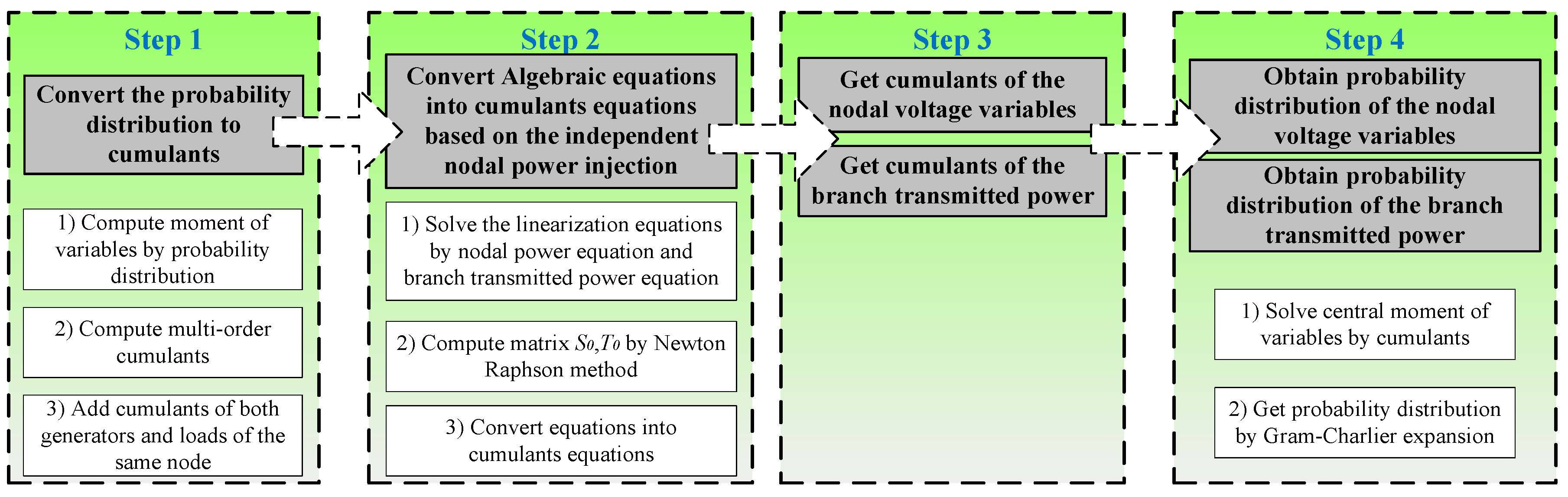
3.2. Novel Probabilistic Load Flow Algorithm Considering Nodal Correlations

For traditional cumulants-based PLF, it is assumed that the nodal injections must be independent of each other. In actual power systems, this situation could not always be true because of the properties of load consumptions, DGs may be associated together by weather related or other factors. Although some studies have been devoted to addressing these correlation problems [11,12,13,14,15], these approaches could not avoid the inverse calculation of Jacobian matrix and full matrix storage and computation, which cost too much computational space and time for large-scale power systems. Therefore, a novel algorithm is proposed in this paper, which can not only take into account of the correlations of the nodal power injections, but also avoid the inverse of the Jacobian matrix to save computational time and storage.

For the novel algorithm, the correlation matrix of the nodal state variables $C_V$ is introduced. This correlation matrix can be obtained by fitting from the historical operation data of the system, or by its relationship to the covariance matrix of the nodal power injections $Co{v}_W$ [30]:

$$\begin{array}{cc}\hfill Co{v}_W& =E\left(\Delta W\Delta W^T\right)-E\left(\Delta W\right)E\left(\Delta W^T\right)\hfill \\ & =E\left(J_0\Delta V\Delta V^T{J}_0{}^T\right)-E\left(J_0\Delta V\right)E\left(\Delta V^T{J}_0{}^T\right)\hfill \\ & =J_{0}E\left(\Delta V\Delta V^T\right)J_0{}^T-J_{0}E\left(\Delta V\right)E\left(\Delta V^T\right)J_0{}^T\hfill \\ & =J_{0}Co{v}_V{J}_0{}^T\hfill \end{array}$$

(41)

where $J_0$ is Jacobian matrix of the system.

Equation (41) can be solved by typical methods of solving linear equations, such as Gaussian elimination or others, and it can avoid the inverse of matrix $J_0$. After solving the covariance matrix $Co{v}_V$, the correlation matrix of the nodal state variables $C_V$ can be obtained.

According to Equations (39) and (40) above, the associated random variable can be calculated by the correlation matrix and the independent variable:

$$\Delta V=L\Delta V_{dl}$$

(42)

where $\Delta V$ and $\Delta V_{\mathrm{dl}}$ are separately the associated and independent vectors for the nodal state variables.

As the random variables of $\Delta V_{\mathrm{dl}}$ are independent, the linearized formula for load flow Equations (12) and (13) can be transformed into the following equations:

$$\Delta W=J_{0}L\Delta V_{\mathrm{dl}}$$

(43)

$$\Delta Z=G_{0}L\Delta V_{\mathrm{dl}}$$

(44)

So the cumulants for the random variables can be expressed as:

$$\Delta W^{\left(k\right)}={\left(J_{0}L\right)}_{•}{}^k\Delta V_{\mathrm{dl}}{}^{\left(k\right)}$$

(45)

$$\Delta Z^{\left(k\right)}={\left(G_{0}L\right)}_{•}{}^k\Delta V_{dl}{}^{\left(k\right)}$$

(46)

where $\Delta W^{\left(k\right)}$, $\Delta V_{dl}{}^{\left(k\right)}$ and $\Delta Z^{\left(k\right)}$ are separately the $k$-th order cumulants of $\Delta W$, $\Delta V_{dl}$ and $\Delta Z$.

Equation (45) can be solved by a typical linear equation-solving method with sparse technology, and Equation (46) can be calculated by simple multiplication of those matrices. Thus it can avoid the inverse of the Jacobian matrix $J_0$ to save computation time and storage.

As $\Delta V_{dl}{}^{\left(k\right)}$ is the $k$-th order cumulant of the independent nodal state variables rather than the actual nodal state variables, so the following calculation should be performed:

$$\Delta V^{\left(k\right)}=L_{•}{}^k\Delta V_{dl}{}^{\left(k\right)}$$

(47)

Through Equation (47), the cumulants calculation for the unknown voltage variables considering the correlations of nodal power injections is finally completed. Then the probability distribution can be obtained by Gram-Charlier series expansion in Equation (28).

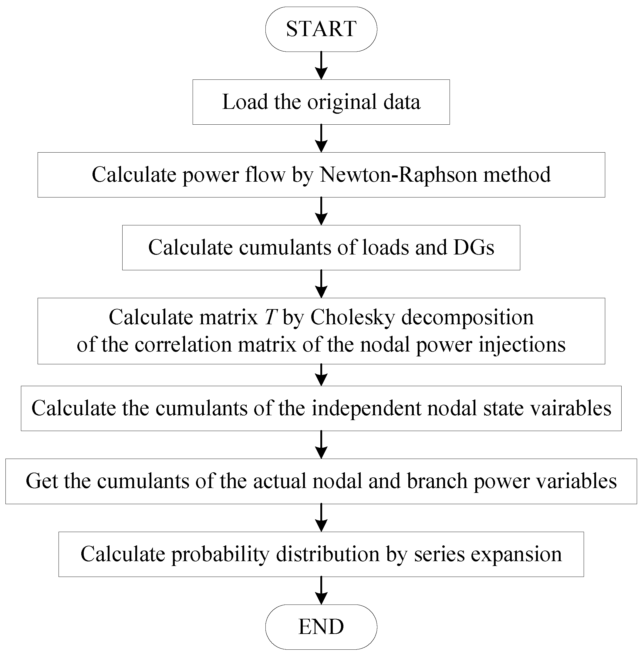
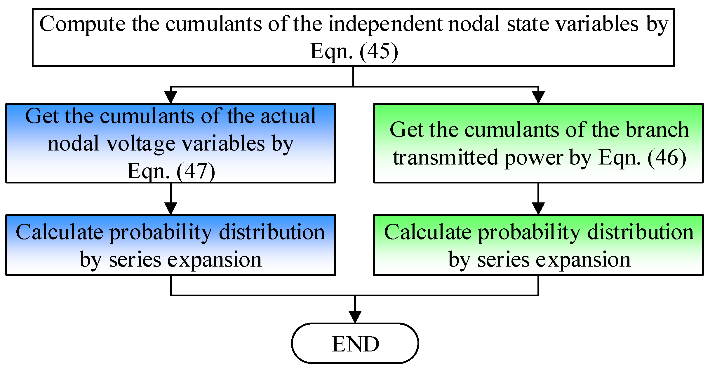
3.3. Flowchart of the Novel Probabilistic Load Flow Algorithm

According to the derivation above, the flowchart of the proposed novel PLF algorithm considering variable correlations is shown in Figure 2.

4. Further Improvement of the Novel Probabilistic Load Flow Based on Parallel Computing

PLF based on serial computing needs to calculate the multi-order cumulants and probability distribution of the nodal voltage variables and the branch transmitted power, which always takes a long time to complete. Parallel computation is therefore introduced into the PLF to improve the computation accuracy and speed of PLF in this section.

4.1. Basics of Parallel Computing

Parallel computing, or called high performance computing, is the combination of parallel computer architecture, parallel algorithm and parallel programming [31]. In this study, the parallel algorithm for the novel PLF considering nodal correlations is developed, the parallel hardware and programming parts are not included.

The evaluating standards are needed to verify the performance of each parallel computing algorithm. The popular evaluating standards include Amdahl’s Law [32], Gustafson’s Law [33], and so on. Typically, the parallel speedup ratio and parallel efficiency are used in these standards, and they are defined as:

$$S_p=\frac{t_c}{t_p}$$

(48)

$$E_p=\frac{S_p}{p}$$

(49)

where $S_p$ and $E_p$ are separately the parallel speedup ratio and parallel efficiency, $t_c$ and $t_p$ are separately the computation time of serial and parallel computation, and $p$ is the number of processors.

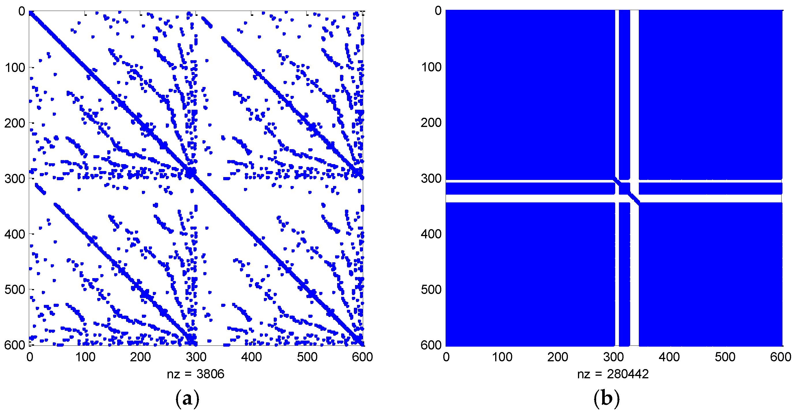
4.2. Parallel Characteristics Analysis for Probabilistic Load Flow Algorithms

According to the uniform partition principle of designing parallel algorithms, the PLF can be divided into two parts: the calculation process of the nodal state variables and the calculation process of the branch transmitted power. For traditional PLF, the two processes are linked to each other because the second part needs the inverse of the Jacobian matrix embedded in the first part. Thus the traditional PLF algorithm can only be parallelized after the inverse of the Jacobian matrix, it would be not so conducive to improve the efficiency of traditional PLF algorithm through parallel computing technology. On the contrary, the two parts of the proposed novel PLF algorithm is generally independent of each other, which makes it suitable for parallel computing.

4.3. Flowchart of the Improved Probabilistic Load Flow Algorithm Based on Parallel Computing

The flow chart of the improved PLF algorithm based on parallel computing is shown in Figure 3, in which the blocks in different colored background can be performed on separate CPU cores, according to the independent Equations (46) and (47).

5. Case Studies

5.1. System Descriptions

In order to validate the accuracy of the novel PLF algorithm, the results from Correlation Latin hypercube sampling Monte Carlo Simulation (CLMCS) [29] are taken as the true values for analytical PLF methods. Both the results of the novel cumulants-based PLF considering nodal correlations and traditional cumulants-based PLF are compared with the true values from CLMCS, all based on the standard IEEE-14 test system [34].

In addition, modified IEEE-300 system, C703 system, and N1047 system [35] with stochastic DGs are used to compare the computing efficiency of the novel PLF algorithm with the traditional cumulants-based PLF algorithm. And the parallel performance is also analyzed accordingly.

The algorithms are coded in MATLAB software (https://cn.mathworks.com/). The simulation hardware consists of a physical memory of 8.00 Gb, and a dual-core CPU i5-3230M (Intel, Santa Clara, CA, USA), with the main frequency of 2.60 GHz. For the parallel test, the MATLAB Parallel Computing Toolbox (PCT) is utilized to realize parallel partitioning for the algorithms.

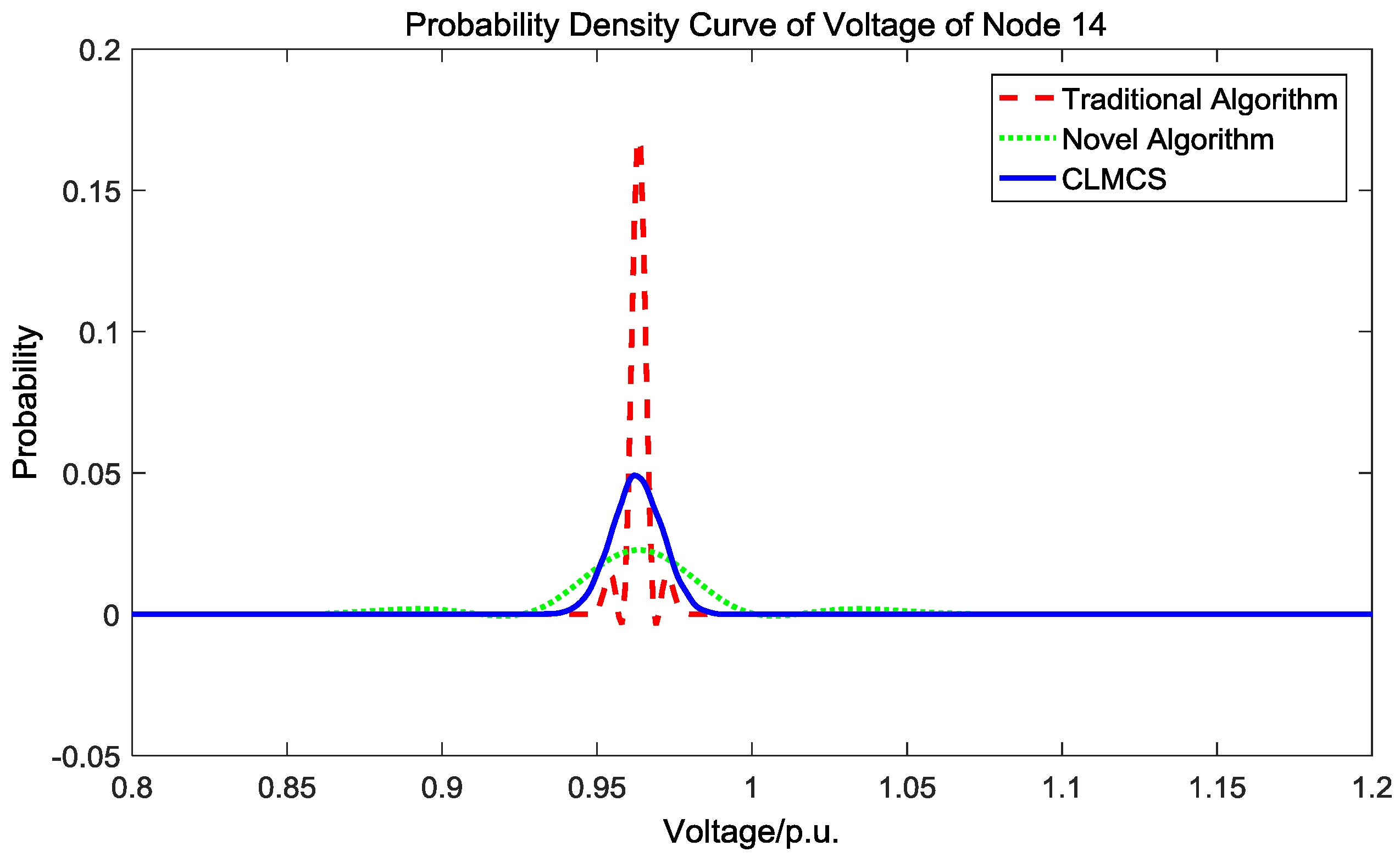
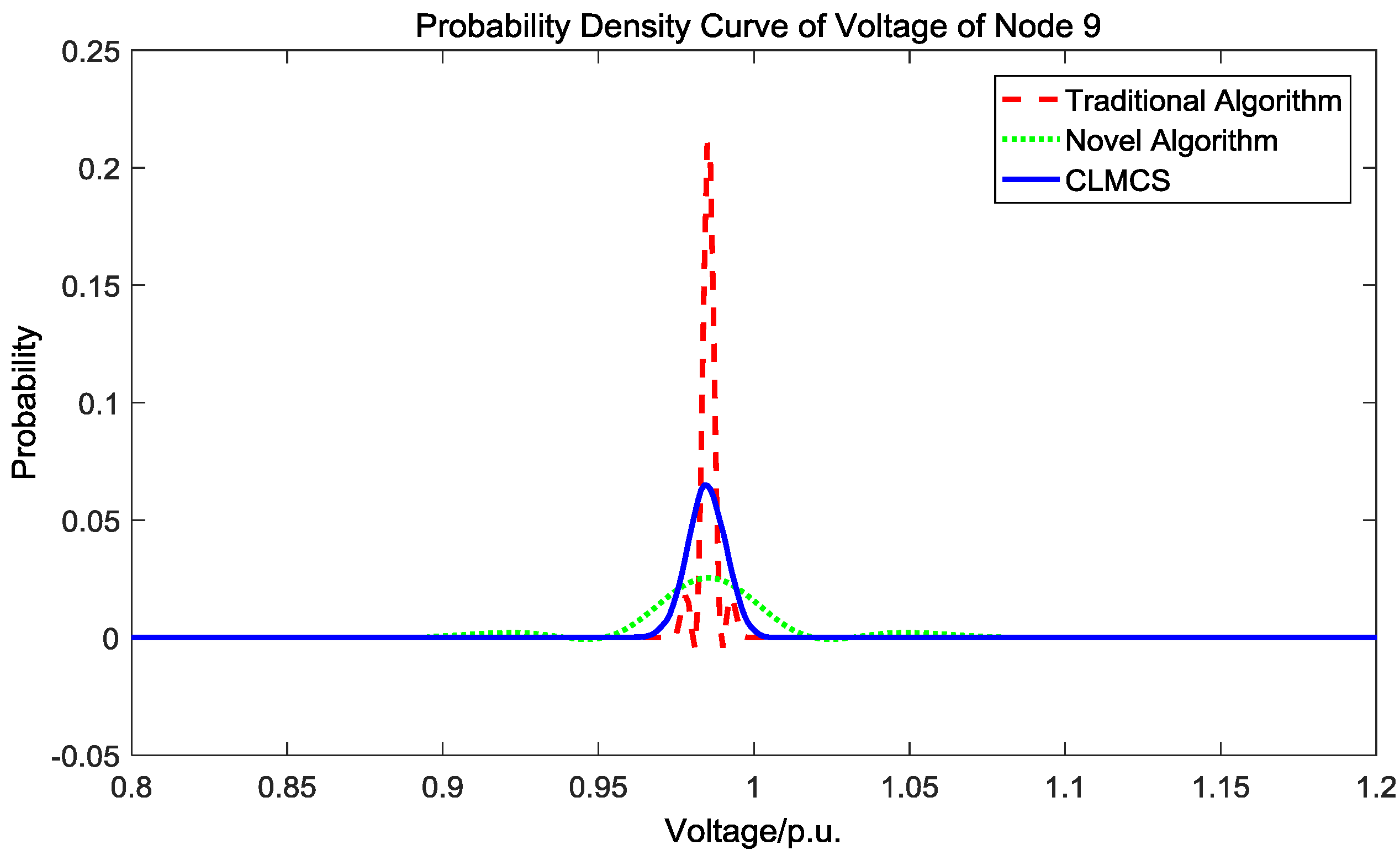
5.2. Accuracy of Novel Probabilistic Load Flow Algorithm

The steady-state operating point of the standard IEEE-14 system is firstly acquired through a normal load flow calculation. The loads are assumed to obey normal distribution, with the steady-state operating points as the mean values, and the variances are all assumed as 0.25% of the means. The correlation coefficient matrix is estimated by the historical data and numerical fitting. Based on these preliminary data, the traditional and novel PLF can then be calculated for the system.

In this case, the probability results based on CLMCS are taken as the true values. And both of the probabilistic distribution results based on the novel and traditional PLF algorithm, are compared with those from CLMCS. Without loss of generality, the probability density curves of the voltages for the load buses 9, 14 are chosen for illustration, which have been shown in Figure 4 and Figure 5.

It can be seen from the probability density curves of voltages by different methods in the Figure 4 and Figure 5 that, both algorithms have the same mean values with the CLMCS method because of the cumulants-based PLF principle, and the novel cumulants-based PLF algorithm is more accurate than traditional PLF algorithm since it has smaller variance error from the true distribution of Monte Carlo-based method. To quantitatively analyze the accuracy of the novel algorithm, the relative variance error (RVE) of both the novel and traditional algorithm to the true values of simulation-based CLMCS method is introduced, and the RVE is defined by the following equation:

$$RVE=\sqrt{\frac{{\displaystyle \sum _{i=1}^n{\left(f_i^{\mathrm{cal}}-f_i^{\mathrm{true}}\right)}^2}}{n}}$$

(50)

where $f_i^{\mathrm{cal}}$, $f_i^{\mathrm{true}}$ are separately the calculated and true values, $n$ is the number of points on the probability density curves. And the RVE for the probability density curve of voltage of node 9 in Figure 4 are separately 0.0062 and 0.0132 for the novel and traditional algorithm. Similarly, the RVE of probability density curve of voltage of node 14 in Figure 5 are separately 0.0047 and 0.0196 for the two algorithms, so the accuracy of the novel algorithm can be seen as quantitatively superior to the traditional algorithm.

Although the traditional algorithm has the smaller variance in the distribution curves of Figure 4 and Figure 5, it does not reflect the exact probability distribution of the system. The traditional PLF algorithm has larger RVE because it could not take into consideration the correlations of the nodal power injections. In contrast, our novel PLF algorithm is able to take account of the correlations among all system nodes, as the CLMCS method does.

5.3. Computational Efficiency of Novel Probabilistic Load Flow Algorithm Considering Nodal Correlations

Further tests on larger systems, namely the modified IEEE-300, C703, N1047-bus systems, are performed to investigate the computational performance of the two analytical cumulants-based PLF algorithms. The loads are still assumed to obey a normal distribution with variance set at 0.25% of the means. DGs are integrated to a particular load bus in the following test systems. Weibull distribution is chosen to model the wind speed changes, with the shape parameter and scale parameter of 2.15 and 9.0. The cut-in speed, rated speed, and cut-out speed are separately 3.5 m/s, 13 m/s and 25 m/s. The installed capacity for the wind power generation is 0.7 per unit (p.u.), with a base of 100 MVA. Beta distribution is chosen for the solar radiation fluctuations, with the mean and variance of radiation of 800 W/m² and 300 W/m², and the max radiation is 850 W/m². The installed capacity for the photovoltaic power generation is set as 1.0 p.u.

Since the wind and photovoltaic power fluctuations also belong to nodal power injections, therefore, it would not influence the applicability of our novel PLF algorithm. And these DGs can be applied to any one node or multiple nodes for the test systems. It should be noted that the system parameters need corresponding modifications if there are associated transformers and/or transmission lines connecting those DGs. Also the steady-state operating point must be re-calculated after the newly installed capacity of DGs.

The two test algorithms with DG integrations are also coded in the MATLAB software. The probability distributions of the nodal state variables and branch transmitted power are also transformed from the cumulants of the random vectors. To compare the algorithms’ numerical performance, the computational time of both algorithms is recorded. As the novel algorithm adds calculation in the correlation analysis, we only compare the time of the linearized equations solving, cumulants calculating, and series expansion probability fitting processes of the unknown variables. And the statistical results are listed in

Table 1. Computational efficiency of traditional and novel probabilistic load flow (PLF) algorithms.

Test Systems	Traditional Algorithm (s)	Novel PLF Algorithm (s)	Computational Efficiency Improvement (%)
IEEE-300	6.373	5.634	13.1
C703	14.109	10.479	34.6
N1047	22.075	16.100	37.1

.

It can be seen from Table 1 that, the novel PLF algorithm has faster computation speed than the traditional PLF algorithm, because the novel algorithm is able to avoid the inverse of the Jacobian matrix to save time. Since the calculation of sparse matrix is much easier than full matrix calculation, the computational efficiency can be improved by 13.1%, 34.6% and 37.1% for the modified IEEE-300, C703 and N1047-bus systems respectively.

As the proposed algorithm takes account of the correlations among all the system nodes, while the traditional algorithm cannot reflect these correlations, the time statistical data in the correlation computation is not included in Table 1, according to the control test principle. The time statistics for the correlation matrix calculation are approximately 0.13, 1.13, 3.18 s under modified IEEE-300, C703, N1047 system separately, which increases a very smaller amount of calculation comparing with the 6.373 s, 14.109 s, 22.075 s of the total PLF calculation process. And the speed improvement of novel algorithm can also be confirmed, with slight reduction in the computational efficiency column.

In addition, the computation time for only the cumulants calculation process of the unknown variables is shown in

Table 2. Computational time for the cumulants calculating process only.

Test Systems	Traditional Algorithm (s)	Novel PLF Algorithm (s)	Computational Efficiency Improvement (%)
IEEE-300	0.428	0.085	403.5
C703	2.244	0.493	355.2
N1047	5.300	1.185	347.3

, in which the results are much clearer to illustrate the performance improvement of our novel PLF algorithm. It can be seen from Section 3 that, the improvement of the computational time of our novel PLF algorithm is mainly due to the avoidance of Jacobian matrix inversion.

Furthermore, the sparseness of the Jacobian and its inverse matrices of IEEE-300 system is shown in Figure 6. It can be drawn from Figure 6 that, there would be 3806 non-zero elements for the Jacobian matrix of the IEEE-300 system, while the quantity would reach a number of 280,442 for the sensitivity matrix. Therefore, the novel PLF algorithm that avoids the inverse of the Jacobian matrix and full array calculation, could potentially save the computation storage and time.

Different testing periods [36] can be used to prove the efficiency of the novel PLF algorithm. In this study, the IEEE-300 system with different probabilistic parameters are also used to further prove the effectiveness and applicability of the novel PLF algorithm. In this case study, the loads are still assumed to obey normal distribution, while the variances are all assumed as 2.5% of the means rather than 0.25%. The mean and variance of solar radiation are separately modified to 817 W/m² and 350.575 W²/m⁴. The shape parameter and scale parameter of the Weibull distribution for wind speed variations are modified to 2.05 and 8.0. The computational times for the IEEE-300 system in this case are separately 6.706 s and 6.007 s for the traditional and novel algorithm. The effectiveness of the proposed PLF algorithm can also be demonstrated.

5.4. Parallel Performance of Novel Probabilistic Load Flow Algorithm

The three larger power systems are also adopted to test the superiority of the parallel performance of the novel PLF algorithm over the traditional PLF algorithm. The parallel speedup ratio $S_p$ and parallel efficiency $E_p$ are used to show quantitatively the parallel indices. Parallel computing is applied to both the traditional and novel PLF algorithms, and the results are separately shown in

Table 3. Parallel Performance of the Traditional PLF Algorithm.

Test Systems	Serial Computation Time (s)	Parallel Computation Time (s)	Parallel Speedup Ratio	Parallel Efficiency (%)
IEEE-300	6.373	4.545	1.402	70.1
C703	14.109	9.075	1.555	77.8
N1047	22.075	15.415	1.432	71.6

and

Table 4. Parallel Performance of Novel PLF Algorithm.

Test Systems	Serial Computation Time (s)	Parallel Computation Time (s)	Parallel Speedup Ratio	Parallel Efficiency (%)
IEEE-300	5.634	3.906	1.442	72.1
C703	10.479	6.361	1.647	82.4
N1047	16.100	9.900	1.626	81.3

.

As shown in the Table 3 and Table 4, parallel computing can greatly improve the calculation speed for both algorithms. The maximum speedup ratio can reach about 1.555-fold faster for the traditional PLF algorithm in the 703-bus system, while it can reach about 1.647 times faster for the proposed new PLF algorithm, using the dual-core CPU processor. The parallel performance of the novel algorithm is proven to be better than the traditional algorithm, because the cumulants calculation processes are more independent of each other for the novel PLF algorithm, which makes it more suitable for parallel computing.

6. Conclusions

Consistent fluctuations of wind, photovoltaic power generation and load consumptions have made the modern power system a more complex dynamic system, and the cumulants-based PLF method is an effective way to analyze the influence of these random factors. However, it is still a big challenge to address the correlations among all the random variables. Although some studies have thought of the wind speed correlations between neighboring wind power plants, the correlations among all the nodal injections to the system level have rarely been studied. Therefore, a novel parallel cumulants-based PLF method considering nodal correlations is proposed in this paper, and it is able to deal with the correlations among all the system nodes, and also avoid the Jacobian matrix inversion and full matrix computation in the traditional cumulants-based PLF methods. In addition, parallel computing is utilized to increase the computation speed. The accuracy of the proposed method is validated by numerical tests on the standard IEEE-14 system, comparing with the results from CLMCS method. The computational efficiency and parallel performance are demonstrated by the tests on the modified IEEE-300, C703, N1047 systems with DG integrations. Simulation results have shown that the proposed parallel cumulants-based PLF method is able to get more accurate results using less computational time and physical memory, and it also has better parallel performance, compared with the traditional cumulants-based PLF algorithm.

References

1. Wang, X.F.; Song, Y.; Irving, M. Modern Power Systems Analysis; Springer: New York, NY, USA, 2008. [Google Scholar]
2. Borkowska, B. Probabilistic load flow. IEEE Trans. Power Appar. Syst. 1974, PAS-93, 752–759. [Google Scholar] [CrossRef]
3. Schilling, M.T.; Leite da Silva, A.; Billington, R.; El-Kady, M. Bibliography on power system probabilistic analysis (1962–1988). IEEE Trans. Power Syst. 1990, 5, 1–11. [Google Scholar] [CrossRef]
4. Da Silva, A.L.; Arienti, V. Probabilistic load flow by a multilinear simulation algorithm. IEE Proc. C Gener. Transm. Distrib. 1990, 137, 276–282. [Google Scholar] [CrossRef]
5. Usaola, J. Probabilistic load flow with wind production uncertainty using cumulants and Cornish-fisher expansion. Int. J. Electr. Power Energy Syst. 2009, 31, 474–481. [Google Scholar] [CrossRef]
6. Morales, J.M.; Perez-Ruiz, J. Point estimate schemes to solve the probabilistic power flow. IEEE Trans. Power Syst. 2007, 22, 1594–1601. [Google Scholar] [CrossRef]
7. Sun, Y.; Mao, R.; Li, Z.; Tian, W. Constant Jacobian matrix-based stochastic Galerkin method for probabilistic load flow. Energies 2016, 9, 153. [Google Scholar] [CrossRef]
8. Zhang, P.; Lee, S.T. Probabilistic load flow computation using the method of combined Cumulants and Gram-Charlier expansion. IEEE Trans. Power Syst. 2004, 19, 676–682. [Google Scholar] [CrossRef]
9. Hernández, J.; Ruiz-Rodriguez, F.; Jurado, F. Technical impact of photovoltaic-distributed generation on radial distribution systems: Stochastic simulations for a feeder in Spain. Int. J. Electr. Power Energy Syst. 2013, 50, 25–32. [Google Scholar] [CrossRef]
10. Sun, C.; Bie, Z.; Xie, M.; Jiang, J. Fuzzy copula model for wind speed correlation and its application in wind curtailment evaluation. Renew. Energy 2016, 93, 68–76. [Google Scholar] [CrossRef]
11. Usaola, J. Probabilistic load flow with correlated wind power injections. Electr. Power Syst. Res. 2010, 80, 528–536. [Google Scholar] [CrossRef]
12. Shi, D.; Cai, D.; Chen, J.; Duan, X.; Huijie, L.I.; Yao, M. Probabilistic load flow calculation based on Cumulant method considering correlation between input variables. Chin. Soc. Electr. Eng. 2012, 32, 104–113. [Google Scholar]
13. Fan, M.; Vittal, V.; Heydt, G.T.; Ayyanar, R. Probabilistic power flow studies for transmission systems with photovoltaic generation using Cumulants. IEEE Trans. Power Syst. 2012, 27, 2251–2261. [Google Scholar] [CrossRef]
14. Morales, J.; Baringo, L.; Conejo, A.; Mínguez, R. Probabilistic power flow with correlated wind sources. IET Gener. Transm. Distrib. 2010, 4, 641–651. [Google Scholar] [CrossRef]
15. Yu, H.; Chung, C.Y.; Wong, K.P.; Lee, H.W.; Zhang, J.H. Probabilistic load flow evaluation with hybrid latin hypercube sampling and cholesky decomposition. IEEE Trans. Power Syst. 2009, 24, 661–667. [Google Scholar] [CrossRef]
16. Villanueva, D.; Feijóo, A.E.; Pazos, J.L. An analytical method to solve the probabilistic load flow considering load demand correlation using the DC load flow. Electr. Power Syst. Res. 2014, 110, 1–8. [Google Scholar] [CrossRef]
17. Barnes, G.H.; Brown, R.M.; Kato, M.; Kuck, D.J.; Slotnick, D.L.; Stokes, R.A. The ILLIAC IV computer. IEEE Trans. Comput. 1968, C-17, 746–757. [Google Scholar] [CrossRef]
18. Torralba, A.; Gomez, A.; Franquelo, L.G. Three methods for the parallel solution of a large, sparse system of linear equations by multiprocessors. Int. J. Energy Syst. 1992, 12, 1–5. [Google Scholar]
19. Lau, K.; Tylavsky, D.J.; Bose, A. Coarse grain scheduling in parallel triangular factorization and solution of power system matrices. IEEE Trans. Power Syst. 1991, 6, 708–714. [Google Scholar] [CrossRef]
20. Alvarado, F.L. Parallel solution of transient problems by trapezoidal integration. IEEE Trans. Power Appar. Syst. 1979, PAS-98, 1080–1090. [Google Scholar] [CrossRef]
21. Chai, J.S.; Bose, A. Bottlenecks in parallel algorithms for power system stability analysis. IEEE Trans. Power Syst. 1993, 8, 9–15. [Google Scholar] [CrossRef]
22. Fang, W.; Ngan, H.W. A robust load flow technique for use in power systems with unified power flow controllers. Electr. Power Syst. Res. 2000, 53, 181–186. [Google Scholar] [CrossRef]
23. Abouzahr, I.; Ramakumar, R. An approach to assess the performance of utility-interactive wind electric conversion systems. IEEE Trans. Energy Convers. 1991, 6, 627–638. [Google Scholar] [CrossRef]
24. Liu, J.; Fang, W.; Yang, Y.; Yang, C.; Lei, S.; Fu, S. Increasing wind power penetration level based on hybrid wind and Photovoltaic generation. In Proceedings of the TENCON 2013—2013 IEEE Region 10 Conference (31194), Xi’an, China, 22–25 October 2013.
25. Karaki, S.; Chedid, R.; Ramadan, R. Probabilistic performance assessment of autonomous solar-wind energy conversion systems. IEEE Trans. Energy Convers. 1999, 14, 766–772. [Google Scholar] [CrossRef]
26. Liu, J.; Fang, W.; Zhang, X.; Yang, C. An improved photovoltaic power forecasting model with the assistance of aerosol index data. IEEE Trans. Sustain. Energy 2015, 6, 434–442. [Google Scholar] [CrossRef]
27. Cai, D.; Chen, J.; Shi, D.; Duan, X.; Li, H.; Yao, M. Enhancements to the cumulant method for probabilistic load flow studies. In Proceedings of the 2012 IEEE Power and Energy Society General Meeting, San Diego, CA, USA, 22–26 July 2012.
28. Ruiz-Rodriguez, F.; Hernandez, J.; Jurado, F. Probabilistic load flow for photovoltaic distributed generation using the Cornish-Fisher expansion. Electr. Power Syst. Res. 2012, 89, 129–138. [Google Scholar] [CrossRef]
29. Chen, Y.; Wen, J.; Cheng, S. Probabilistic load flow analysis considering dependencies among input random variables. Proc. CSEE 2011, 31, 80–87. [Google Scholar]
30. Wang, K.; Tse, C.; Tsang, K. Algorithm for power system dynamic stability studies taking account of the variation of load power. Electr. Power Syst. Res. 1998, 46, 221–227. [Google Scholar] [CrossRef]
31. Chen, G.-L.; Sun, G.-Z.; Zhang, Y.-Q.; Mo, Z.-Y. Study on parallel computing. J. Comput. Sci. Technol. 2006, 21, 665–673. [Google Scholar] [CrossRef]
32. Amdahl, G.M. Validity of the single processor approach to achieving large scale computing capabilities. In Proceedings of the Spring Joint Computer Conference, Atlantic City, NJ, USA, 18–20 April 1967; pp. 483–485.
33. Gustafson, J.L. Reevaluating Amdahl’s law. Commun. ACM 1988, 31, 532–533. [Google Scholar] [CrossRef]
34. Duan, C.; Jiang, L.; Fang, W.; Liu, J. Moment-SOS approach to interval power flow. IEEE Trans. Power Syst. 2016. [Google Scholar] [CrossRef]
35. Niu, S.; Wang, J.; Huo, C.; Liu, J. An novel power flow calculation model with the elimination of interconnecting nodes. In Proceedings of the First International Conference on Information Sciences, Machinery, Materials and Energy, Chongqing, China, 11–13 April 2015.
36. Ruiz-Rodriguez, F.; Hernández, J.; Jurado, F. Voltage unbalance assessment in secondary radial distribution networks with single-phase photovoltaic systems. Int. J. Electr. Power Energy Syst. 2015, 64, 646–654. [Google Scholar] [CrossRef]
Figure 1. Block diagram for the traditional probabilistic load flow (PLF) algorithm.
Energies 09 01041 g001
Figure 2. Flowchart of novel PLF algorithm considering nodal correlations.
Energies 09 01041 g002
Figure 3. Flowchart of the improved PLF algorithm based on parallel computing.
Energies 09 01041 g003
Figure 4. Probability density curves of voltage for node 9. p.u.: per unit.
Energies 09 01041 g004
Figure 5. Probability density curves of voltage for node 14.
Energies 09 01041 g005
Figure 6. The sparseness of the Jacobian matrix and its inverse of IEEE-300 systems. (a) the Jacobian matrix; (b) the inverse of the Jacobian matrix.
Energies 09 01041 g006