Article

A Novel Approach for Microgrid Protection Based upon Combined ANFIS and Hilbert Space-Based Power Setting

by
Ali Hadi Abdulwahid
1,2,* and
Shaorong Wang
1
1
School of Electrical and Electronic Engineering, Huazhong University of Science and Technology, Wuhan 430074, China
2
Department of Engineering Electrical Power, Engineering Technical College, Southern Technical University, Basrah 61001, Iraq
*
Author to whom correspondence should be addressed.
Energies 2016, 9(12), 1042; https://doi.org/10.3390/en9121042
Submission received: 20 September 2016 / Revised: 10 November 2016 / Accepted: 30 November 2016 / Published: 10 December 2016

Abstract

:
Nowadays, the use of distributed generation (DG) has increased because of benefits such as increased reliability, reduced losses, improvement in the line capacity, and less environmental pollution. The protection of microgrids, which consist of generation sources, is one of the most crucial concerns of basic distribution operators. One of the key issues in this field is the protection of microgrids against permanent and temporary failures by improving the safety and reliability of the network. The traditional method has a number of disadvantages. The reliability and stability of a power system in a microgrid depend to a great extent on the efficiency of the protection scheme. The application of Artificial Intelligence approaches was introduced recently in the protection of distribution networks. The fault detection method depends on differential relay based on Hilbert Space-Based Power (HSBP) theory to achieve fastest primary protection. It is backed up by a total harmonic distortion (THD) detection method that takes over in case of a failure in the primary method. The backup protection would be completely independent of the main protection. This is rarely attained in practice. This paper proposes a new algorithm to improve protection performance by adaptive network-based fuzzy inference system (ANFIS). The protection can be obtained in a novel way based on this theory. An advantage of this algorithm is that the protection system operates in fewer than two cycles after the occurrence of the fault. Another advantage is that the error detection is not dependent on the selection of threshold values, and all types of internal fault can identify and show that the algorithm operates correctly for all types of faults while preventing unwanted tripping, even if the data were distorted by current transformer (CT) saturation or by data mismatches. The simulation results show that the proposed circuit can identify the faulty phase in the microgrid quickly and correctly.

1. Introduction

The use of renewable energy sources such as wind power, solar cells, and fuel cells in a microgrid provides a solution to the problem of greenhouse gases, increasing demand for energy sources, and depletion of fossil fuel-based energy. Despite the many benefits of the integration of the microgrid with DG, including the ability to work in an islanded mode, protection challenges have become a source of great concern when the conventional relays’ performance degrades and stop working. The protection relay faces serious challenges because the microgrid works with different types of DGs, including induction-, synchronous-, and inverter-based on DGs. The magnitude of the fault current varies greatly according to the type of contribution of the DG to the fault.
This occurs because of the limited current of inverter-based DGs. In addition, the operating conditions may change the network topology of the microgrid to provide consumers with quality and reliable energy. Under these operating conditions, it is expected that there would be major differences in the fault current. Because of the bidirectional flow of energy through the microgrid, it is necessary to use selective and reliable relays placed at the end of the feeder. Consequently, overcurrent relays (OC) with a fixed setting fail to provide accurate and reliable protection to the microgrid [1,2,3,4,5,6,7].
The paper is organized into six sections. Section 2 reviews the technical challenges of the protection of a microgrid. Section 3 the proposed algorithm for the system with (ANFIS) for the protection. Section 4 discusses the implementation of the proposed protection. Section 5 describes the Simulation and Analysis. Finally, Section 6 presents conclusions.

2. Protection Challenges

In general, a microgrid can operate in either network-connected or islanded mode, where the microgrid is interfaced with the main system of power by a fast switch called a static switch (SS). The philosophy of protection is to have the same protection strategies for operating in both island mode and the connected grid. The static switch is designed to open up all the faults. This is essential to protect the microgrid in both systems on the grid-connected and islanded mode of operation, against all types of faults.
The problem comes in islanded operation when inverter fault current sources are limited by the rating. Faults in island-based investor’s microgrid currents may not have sufficient quantities using traditional techniques of over-current protection. Faults within the microgrid need to be cleaned up with techniques that do not depend on the high currents of the fault. This possibility requires an expanded protection strategy. The microgrid assumes that the sources have appropriate qualifications to meet the demands of the load in islanded mode [8,9,10].
In this work, we presented a formulation of the generalized theory of instantaneous reactive power. This new formulation proposes a way to calculate the instantaneous reactive power that can be applied not only to three-phase power systems but to multiphase power systems. This theory is very efficient and flexible in the design of controllers for power conditioners, which are based on power electronic devices.
The integration of a microgrid into the major network raises significant questions about the benefit of using the traditional techniques of protection, which require an intelligent adaptive process. The technical challenges that must be overcome in the design of the system of protection of the microgrid, to enable it to operate successfully, are as follows:

2.1. Bidirectional Current Flow

The integration of the microgrid with the active distribution network, to provide the energy supply to local loads in the microgrid is also expected to export energy to the network with increasing production, which makes the power flow in the opposite direction [4].

2.2. Frequent Changes in Microgrid Configuration

These changes are either because of the integration or disconnection of branches in the network. The current magnitude faults could be affected by any changes in the configuration of the microgrid. The frequent changes in the short-circuit fault current make OC relays more complicated. These relays must modify their tripping characteristics immediately regarding any change in the configuration of the network [4].

2.3. Reduction in Short Circuit Fault Current Level

Current sharing of a fault at the main grid and the microgrid reduces the fault current for any relay. In addition, DG based on converter power electronics limits the short circuit fault current level, especially in the operation of the island mode [4].

2.4. Selectivity and Sensitivity of an Overcurrent Relay

The protection system must be able to make a distinction between main grid and microgrid faults [11,12,13,14,15,16,17,18]. In faults of the main grid, it is necessary to carry out islanding to protect the microgrid. When faults occur, the protection system should only isolate the smallest faulted section. Thus, the protection system should be able to operate selectively with regard to any faults, or to disconnect the faulted section. The sensitivity of the relay must be adjusted without affecting the selectivity of the protection system.

2.5. Fast and Reliable Communication in the Case of Adaptive Protection System

This is the main problem in the design of the protection system microgrid. Online monitoring and calculation of the short circuit fault current level are required for each small change in the configuration of the grid for the proper adaptive functioning of any protection system. This requires the application of a fast and reliable method and robust communication with a backup system.

3. Proposed Protection Scheme

To increase the reliability of a power system, many factors can cause failure of protection and there is always a possibility of a failure of the Circuit Breaker (CB). For this reason, it is necessary to supplement the primary protection strengthened by the backup protection in the network and make sure that nothing can prevent elimination of a failure of the system. The proposed protection scheme consists of two main stages. The proposed protection scheme consists of two main stages. The mainly used HSBP algorithm to identify the fault as primary protection and promotion by the method of THD detection used to complement the performance of the backup protection and then the second stage works ANFIS as a decision maker send to run the circuit breaker. As a result, the relay will trip and isolate the faulted section, leaving the rest of the network unaffected. The faulted phase can then be identified very clearly. Variation of the fundamental is used to identify the fault. As will be seen from the results presented in the next section, it is important to emphasize that HSBP could be applied to both instantaneous values as well as the phasors [11]. The ANFIS is a fuzzy Sugeno model of integration, where the final fuzzy inference system output is optimized through the training of ANNs. ANN has a good capacity of pattern recognition. It was concluded from a theoretic analysis that a perception neuron could realize protection based on ratio HSBP theory. Furthermore, a multi-layer ANN of protection model was advanced that was characterized by non-liner theory.

3.1. Proposed Algorithm of Hilbert Space-Based Power (HSBP) for Protection

The instantaneous reactive power theory, also named the “p-q” formulation, as introduced by Akagi in [19,20], is based on the Clarke coordinates transformation. The voltage and current vectors in phase coordinates corresponding to a three-phase system are expressed as follows:
u = [ u a u b u c ] T .   i = [ i a i b i c ] T .
Three-phase instantaneous voltage and current can be expressed as instantaneous space vectors. Applied to the voltage and current vectors in A-B-C phase coordinates, they can be transformed into αβ0 orthogonal coordinates through transformation. The new coordinates system is based on a transformation using Equations (2) and (7) [19]:
[ α β 0 ] = 2 3 [ 1 1 2 1 2 0 3 2 3 2 1 2 1 2 1 2 ] [ a b c ]
Equations (3)–(6) define the three power variables that are applied to the voltage and current vectors in phase coordinates: zero-sequence instantaneous real power p 0 , instantaneous real power p α β , and instantaneous imaginary power q α β :
p 0 ( t ) = u 0 i 0
p α β ( t ) = [ u α u β ] [ i α i β ] = u α i α + u β i β
q α β = q α β ( t ) = [ u α u β ] T [ i α i β ] T
q α β = ( u β i α + u α i β )
The “p-q” formulation defines the generalized instantaneous power p ( t ) and instantaneous reactive power vector q ( t ) in terms of the α β 0 components. The instantaneous active and reactive power of the three phases can be defined as follows. From this equation, the current may be expressed according to the power quantities:
[ p 0 p α β q α β ] = [ u 0 0 0 0 u α u β 0 u β u α ] [ i 0 i α i β ]
where
u α β 2 = u α 2 + u β 2
On the other hand, if currents and power levels are known variables, voltages can be given by applying the inverse matrix in Equation (4). For the instantaneous current in αβ orthogonal coordinates and the instantaneous active current and instantaneous reactive current in αβ orthogonal coordinates, the following expressions are given by these procedures:
[ i α i β ] = 1 u α 2 + u β 2 [ u α u β u β u α ] [ p q ]
[ u α u β ] = 1 i α 2 + i β 2 [ i α i β i β i α ] [ p q ]
The instantaneous voltage and current of the three-phase system are generally regarded as periodic functions of time, so that we can build a periodic function of space as follows:
X 3 = { ( f 1 ( t ) , f 2 ( t ) , f 3 ( t ) ) T }
t R , f i ( t ) = f i ( t ± T ) ,   i = 1 , 2 , 3 , T R
Then, with the three-phase instantaneous voltage vector u and instantaneous current vector i   u , i X 3 , the inner product in the periodic function space X 3 is defined as follows:
u , i = 1 T 0 T ( u a ( t ) i a ( t ) + u b ( t ) i b ( t ) + u c ( t ) i c ( t ) ) d t
The norm of X 3 is defined as:
u = u , u
The periodic function space X 3 becomes the inner product space and Hilbert space. Analogously, the n-dimensional periodic function space is constructed as Equation (13) to the n-phase system:
X n = { ( f 1 ( t ) , f 2 ( t ) , f n ( t ) ) T }
t R , f i ( t ) = f i ( t ± T ) ,   i = 1 , 2 , 3 , , n , T R
and n-phase instantaneous voltage vector u and instantaneous current vector i, u , i X n ,
u = [ u 1 ( t ) u 2 ( t ) u n ( t ) ]   i = [ i 1 ( t ) i 2 ( t ) i n ( t ) ]
The inner product and norm in n-dimensional periodic function space X n are defined as:
u , i = 1 T 0 T l = 1 n u 1 ( t ) i 1 ( t ) d t
u = u , u
Therefore, the n-dimensional periodic function space X 3 becomes the n-dimensional inner product space and Hilbert space. In n-dimensional Hilbert space, according to the principle that the active current is the component of phase current that has the minimum average capacity for work, the active current vector i p is defined as the projection of the phase current vector i to the phase voltage vector u as Equation (16) [21].
i p = [ i p 1 ( t ) , p 2 ( t ) , , p n ( t ) , ] T = u ( t ) i ( t ) u ( t ) u ( t ) u ( t )
i p = 1 T 0 T l = 1 n u 1 ( t ) i 1 ( t ) d t 1 T 0 T l = 1 n u 1 2 ( t ) d t u ( t )
The active power P is defined as the product of the norm of the phase voltage vector u and the norm of the active current vector i p :
P = u i p
The reactive power Q is defined as the product of the norm of the phase voltage vector u and the norm of the reactive current vector i q :
Q = u i q
The apparent power S is defined as the product of the norm of the phase voltage vector u and the norm of the phase current vector i :
S = u i
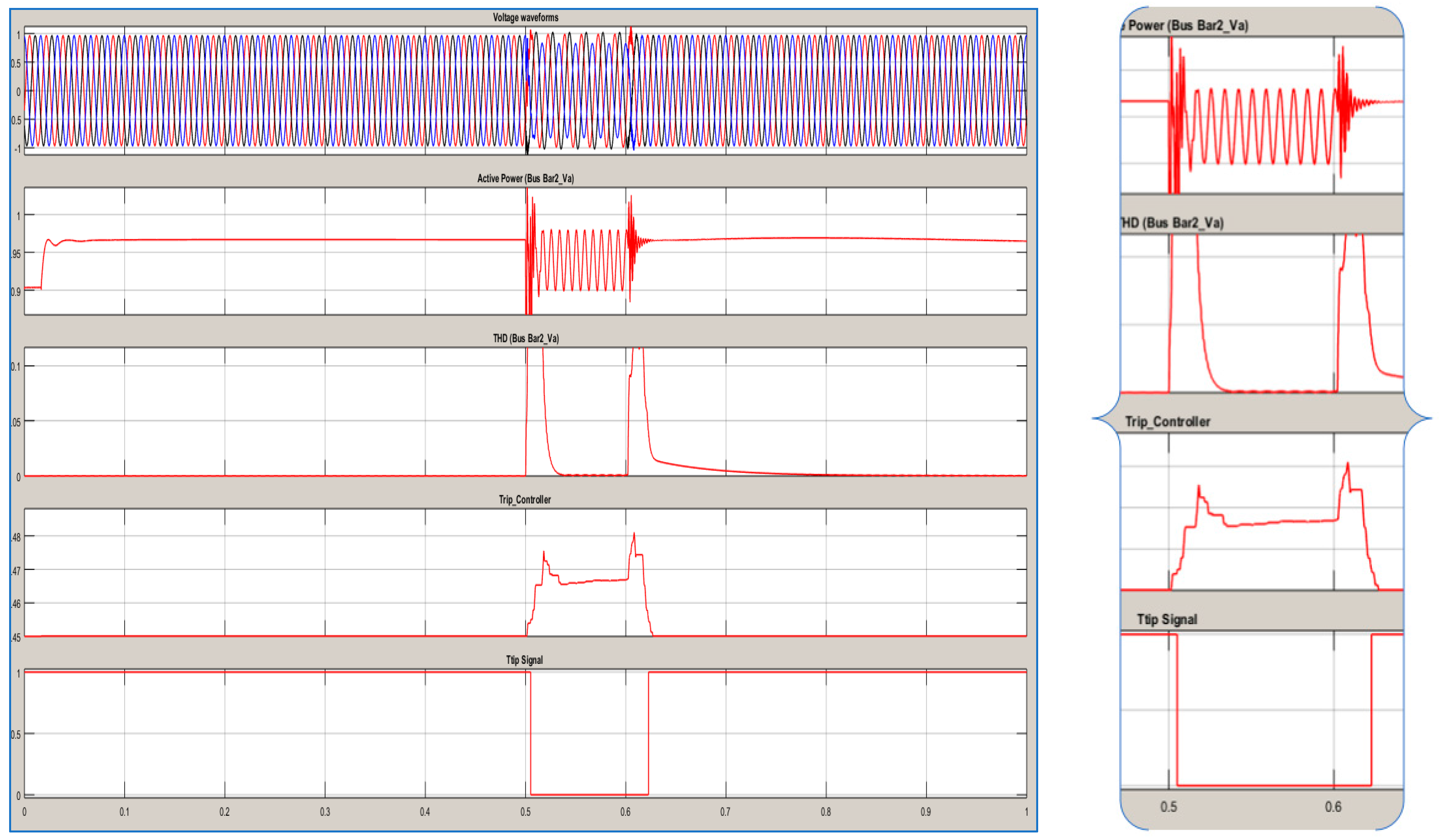
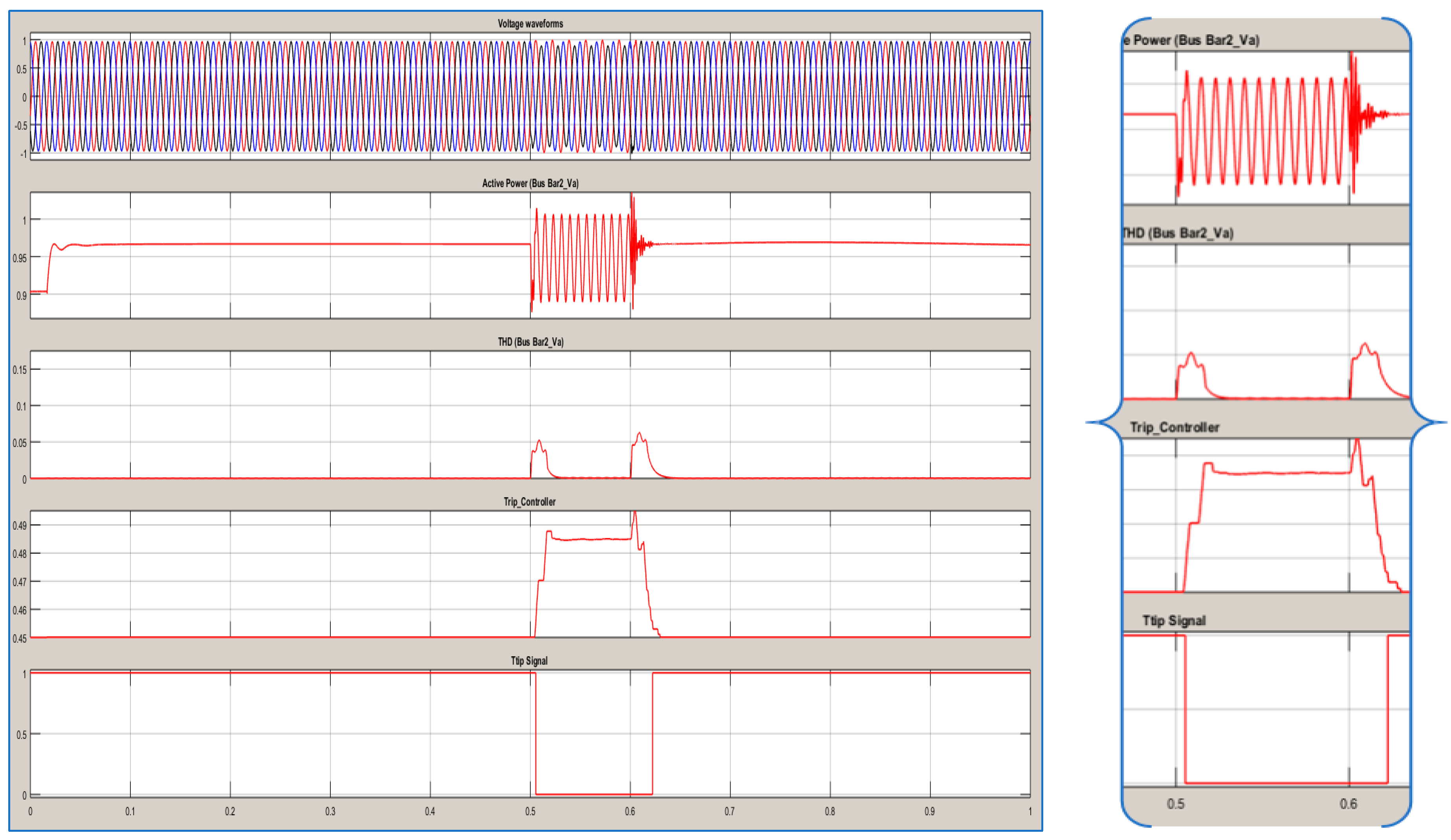
Any disturbance to the main input voltage is reflected as a disturbance in the “p-q” values. Using the disturbed “p-q” values, it is possible to extract the disturbance signal that represents the deviation of the voltage input network.

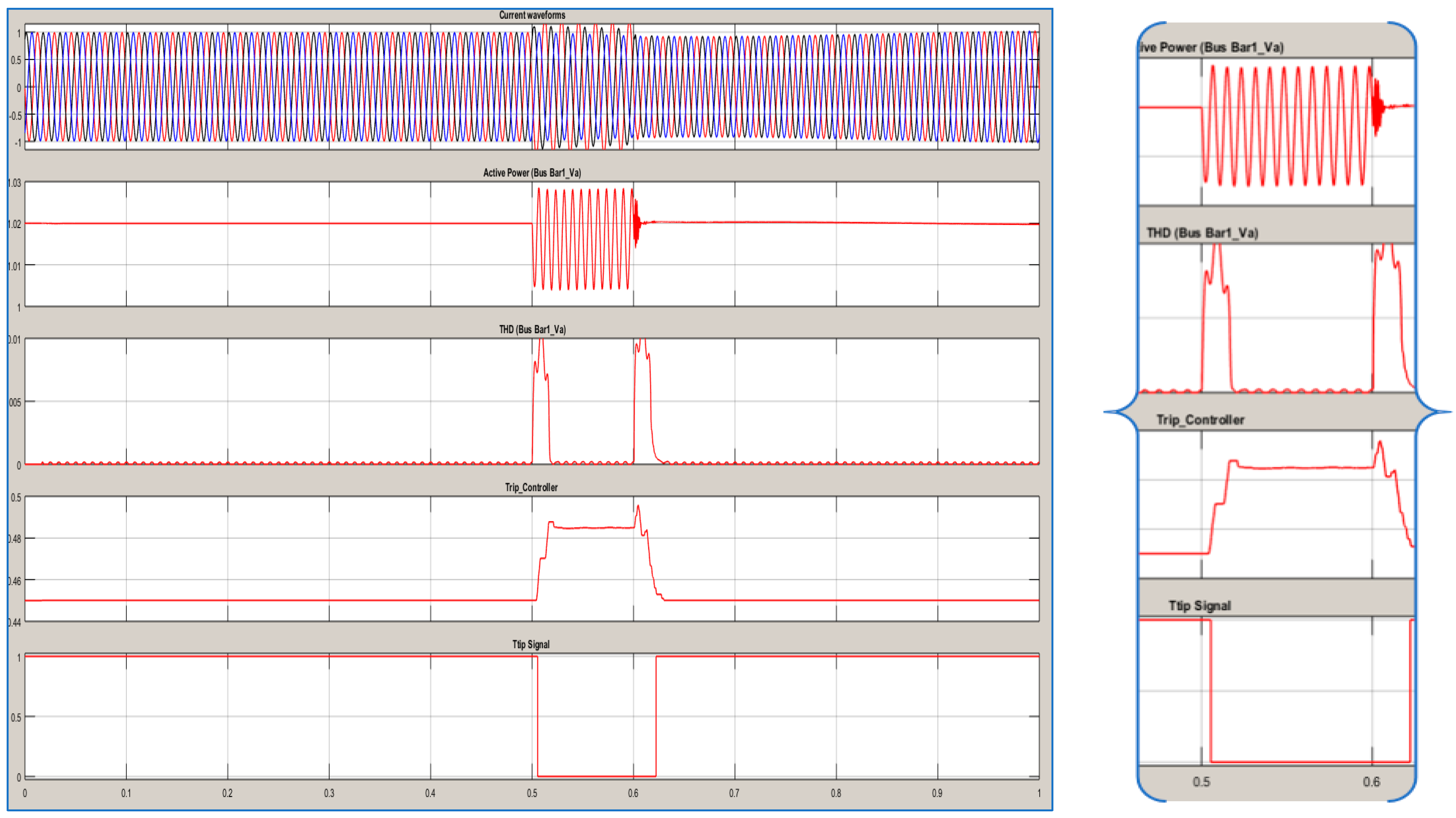
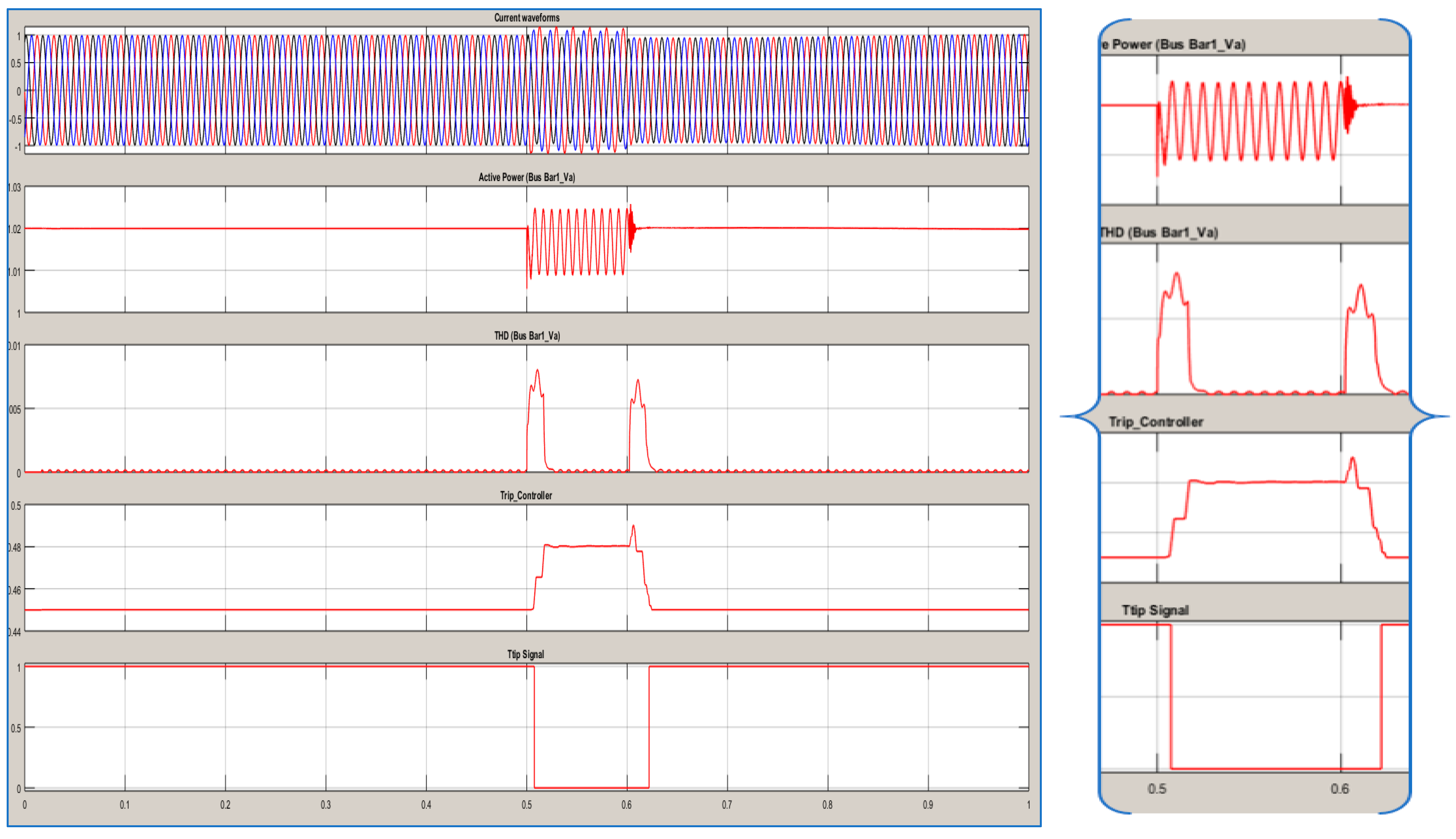
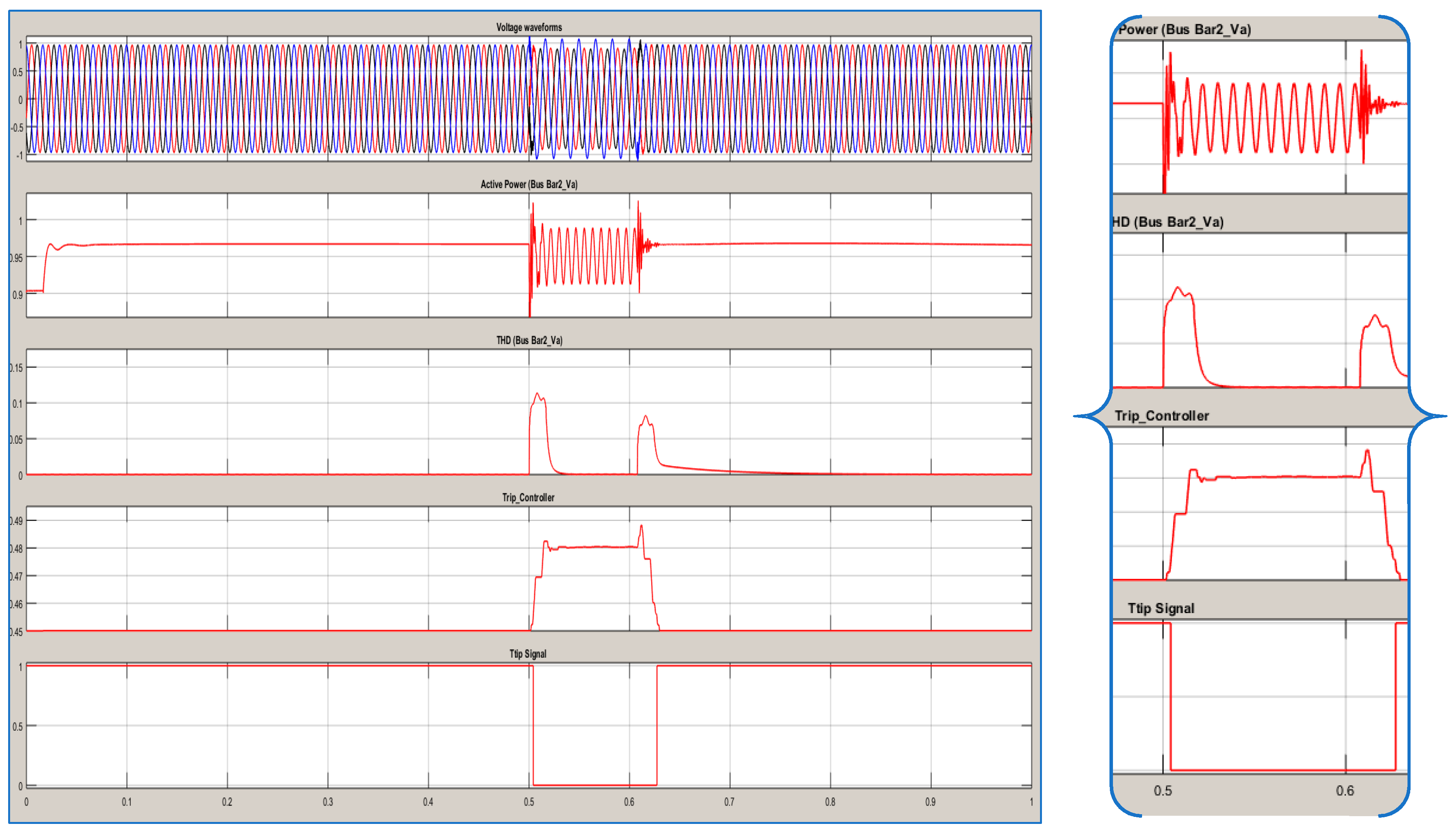
3.2. THD Detection Method

When a fault occurs in the microgrid, it causes distortions in the current. It can be expressed as the total harmonic distortion (THD) of the current at the monitoring time t as in Equation (22):
T H D t = h = 2 H I h 2 I 1 × 100
where I h is the r.m.s. the value of the harmonic components h, and I 1 is the r.m.s. value of the fundamental component [21]. THD variation (ΔTHDt) is a measure of how much the monitored THD at time t deviates from the steady state normal loading conditions, where T H D reference value for the steady state. The average of T H D t over one cycle is defined as follows:
Δ T H D t = T H D a v g , s T H D a v g , t T H D a v g , s × 100 a n d T H D a v g , t = 1 N i = 0 N 1 T H D t i
where T H D a v g , s is the T H D reference value for the steady state and normal loading conditions, and N is the sampling number of one cycle [22].

3.3. Proposed Neuro Fuzzy Inference System for Protection

ANN has strong capabilities of learning at the numerical level. Fuzzy logic has good interpretability and also integrates expert knowledge. The hybridization of both produces learning abilities, good comprehension, and the incorporation of prior knowledge. ANN can be used to learn the values of membership of the fuzzy systems, to build IF-THEN rules, or to build the logic of the decision. The true scheme of the two paradigms is a hybrid fuzzy neural system, which captures the merits of both systems. A neuro-fuzzy system has a neural network architecture built from fuzzy reasoning. Structured knowledge is organized as fuzzy rules, while the capacities of adaptation and learning of neural networks are maintained.
Expert knowledge can increase learning speed and the precision of the estimate. Fuzzy logic is one of the most popular applications in the field of control technology that may be used to control various parameters in real time. This logic, combined with the neural network model, has given very good results. The combined technique of the learning capacity of the NN and the representation of knowledge of FL has created a new hybrid technique called neuro-fuzzy networks [22].
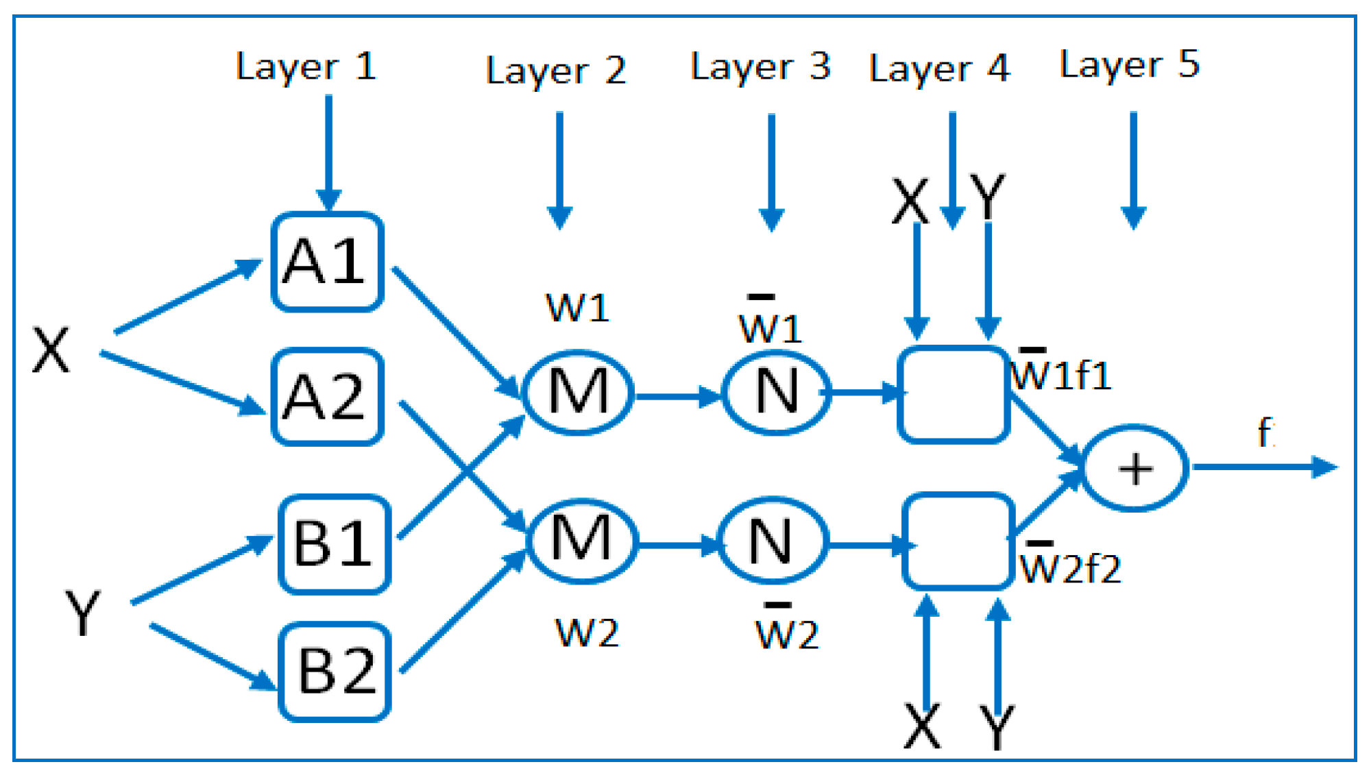
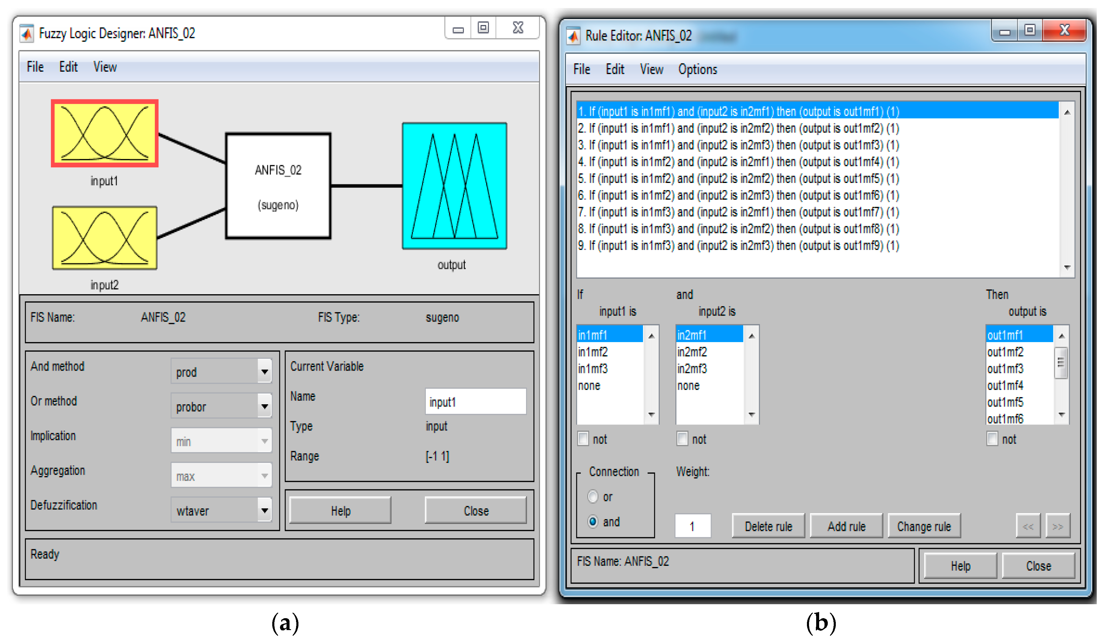
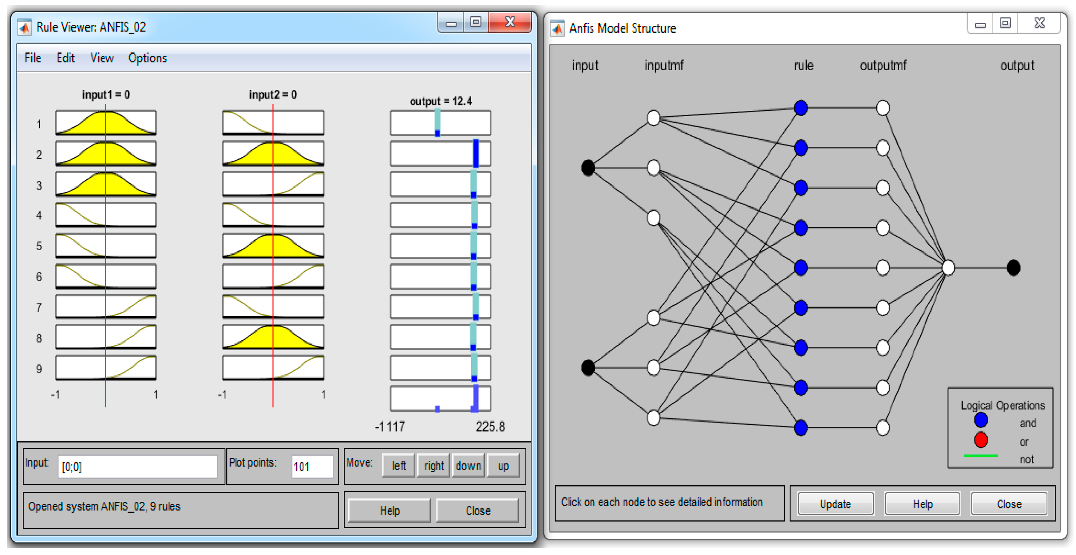
This technique was developed in the early 1990s. Adaptive network-based fuzzy inference system is a combination of neural networks with fuzzy logic; this combination has the explicit knowledge representation of a fuzzy inference system (FIS) learning the ANNs. FIS provides a useful framework for computing based on the concepts of fuzzy theory, fuzzy set if, then rules and fuzzy logic. ANFIS is an FIS applied in the context of an adaptive fuzzy neural network. The main goal is to optimize the parameters of an equivalent FIS using a learning algorithm with input datasets for output. Optimization of the parameters is performed in such a way as to minimize measurement errors. A typical architecture of an ANFIS for two inputs is shown in Figure 1, in which the circle indicates a fixed node while the square indicates an adaptive node [23,24].
For two inputs (x and y) and one output (f), in the first layer, the input values of the universe are converted into their respective membership values by the corresponding membership functions. Here, the membership function can be any appropriately membership function, such as a generalized bell function as in Equation (27), where { a i , b i ,   c i } is a set of parameters called a parameter premise [23].
Rule 1: IF x is A1 and y is B1, then
f 1 = p 1 x + q 1 y + r 1
Rule 2: IF x is A2 and y is B2, then
f 2 = p 2 x + q 2 y + r 2
(A1, A2, B1, B2) are called the premise parameters.
(pi, qi, ri) are called the consequent parameters, i = 1, 2.
The consequent parameters (p, q, and r) of the nth rule contribute through a first-order polynomial within the fuzzy region specified by the fuzzy rule; pn, qn, and rn are the design parameters that are determined during the learning process.
Layer 1: Generate the membership grades: adaptive nodes, the outputs of this layer, are the fuzzy membership grade of the inputs.
O 1 , i = μ A i ( x )       i = 1 ,   2 O 1 , i = μ B i 2 ( y ) i = 3 ,   4
where O1,i is the membership function. In this layer the parameters of each MF are adjusted. μ A i ( x ) and μ B i ( x ) are any appropriately parameterized membership functions.
μ A i ( x ) = { 1 + [ ( x c i ) 2 a i 2 ] b i } 1
Layer 2: Generate the firing strengths. The nodes are fixed nodes with function of multiplication.
O 2 , i = w i = μ A i ( x ) × μ B i ( x )   i = 1 ,   2
Layer 3: Normalize the firing strengths. The nodes are also fixed nodes with function of normalization.
O 3 , i = w ¯ i = w i w 1 + w 2   i = 1 ,   2
Layer 4: Calculate rule outputs based on the consequent parameters:
Each node in this layer is an adaptive node and in this layer parameters of output are adjusted.
O 4 , i = w ¯ i f i = w ¯ i ( p i x + q i y + r i )
Layer 5: Add up all the inputs from layer 4: a fixed node with the function of the summation:
O 5 , 1 = i w ¯ i f i
when input–output training patterns exist, the weight vector (w), which consists of the consequent parameters, can be solved by using a regression technique.

4. Implementation of the Proposed Protection Scheme

As can be seen in Figure 2, the modeled microgrid is connected to the main grid by means of a 24.9 kV Dyn transformer. It also includes one photovoltaic array (800 kW), one wind farm (9 MW), and a solid oxide fuel cell stack (150 kW), which are interfaced with the network through respective YNyn transformers. Detailed models of components used in the microgrid are given in the Appendix A.
The Simulink model with the ANFIS for the proposed protection of the microgrid was developed in Matlab, as shown in Figure 2. In order to start the simulations, the nine fuzzy rule set must first be invoked from the command window in Matlab [10].
In Figure 3, the input data are measured based on the generalized theory of instantaneous reactive power values are calculated for active and reactive power to A-B-C phase. The outputs from the primary protection and backup protection used to discriminate the healthy states and/or defective.
In Figure 4, the sample model demonstrated here on the active/reactive power vector magnitude normalization, the output parameters derived are sent to the end of the feeder in the busbar. The output becomes active when the fault occurs. After acquiring the required data, they are processed using the decision maker, ANFIS employs the theory of fuzzy sets and fuzzy if-then rules to derive outputs. The ANFIS for fault detector output is indexed with either the presence of a fault the non-faulty situation. The main objective of using the ANFIS method herein is to identify the occurrence of faults accurately and quickly in the microgrid model.
If the output of the decision maker is higher than the 0.5, the trip signal sends to the CB. It is important to emphasize that the proposed adaptive network-based fuzzy inference system computes each different power component independently.

Applications of ANFIS Network for Protection Network

The structure was built in Matlab (R2015a). The fuzzy inference method used is Sugeno, because it gives better results than the Mamdani method in designing. The type of membership functions was interrogated before choosing the best one: built-in function triangular (gaussian) membership. The trial-and-error approach for designing the ANFIS model, i.e., selecting the type of interference, the composition function type, and the number of the membership functions in the hidden layer, gave excellent results, i.e., the minimum number of rules and easy simulation. Figure 5 and Figure 6 show the Matlab fuzzy procedure based on the design toolbox Appendix B.
The ANFIS method builds a fuzzy inference system (FIS) whose membership function parameters are tuned (adjusted) using least-squares estimation and the back propagation algorithm. This enables fuzzy systems to learn from the data provided by the model. The fuzzy inference structure of the system lies in the types of network structures, similar to that of neural networks, which map the inputs with an input membership functions and related parameters, and then pass through the output membership functions and associated parameters to the results [23,24].
The process design of a sensor fault using ANFIS through the following steps:
  • Step 1: Generate suitable training data. Due to the limited amount of practical, data fault, it is necessary to generate data training/testing using simulation.
  • Step 2: Choose the ANFIS structure suitable for a particular application.
  • Step 3: The training ANFIS.
In this step, the data collected in Step (1) are presented as input data into ANFIS. It has been trained various network configurations in order to create a suitable network with satisfactory performance. ANFIS are trained to detect a fault. The structure of ANFIS is shown in Figure 5. The parameters are selected in such a way that the optimization method is hybrid, the MF type is gbellmf (generalized bell-shaped membership function), the linear output is membership function, the error tolerance is 0.01, the number of epochs is 100, grid partitions, the inputs of the grid partitions number 3, and the output is MF type, defined to be constant.
  • Step 4: Assess the ANFIS trained using test patterns so that their performance is satisfactory.
When the production of test patterns and the error of the network reaches an acceptable range, the fuzzy system is regulated in the best state, which means that membership functions and fuzzy rules achieve good fitting.
The parameters taken into account for each type of fault are:
Fault type, (AG, BG, CG, AB, BC, CA, AB-G, BC-G, CA-G, and ABC).
Fault location Lf (km), (10)
Fault impedance Rf (Ω), (1:10:20)
Fault time (s), (0.5, 0.6)
Ideally, the desired output of ANFIS is “1” or “0”. Simulation results using data from the power system model are presented in this section. ANFIS parameters are corrected through training (similar to a neural network). Figure 6 shows the structure of an ANFIS with two inputs and one output. The ANFIS has the following design parameters:
Type: Sugeno,
Gaussian and Generalized bell-shaped membership functions,
Three linguistic terms for each input membership function,
Nine linear terms of output membership functions,
Nine rules (resulting from the number of inputs and membership function terms),
Fuzzy operators: product (and), maximum (or), product (implication), maximum (aggregation), and average weight. There are nine rules, which are sufficient to assign a detector using ANFIS. Some of these rules are as follows:
1.
If (Input1 is in1mf1) and (Input2 is in2mf1) then (Output is out1mf1) (1)
2.
If (Input1 is in1mf1) and (Input2 is in2mf2) then (Output is out1mf2) (1)
3.
If (Input1 is in1mf1) and (Input2 is in2mf3) then (Output is out1mf3) (1)
4.
If (Input1 is in1mf2) and (Input2 is in2mf1) then (Output is out1mf4) (1)
… …
9.
If (Input1 is in1mf3) and (Input2 is in2mf3) then (Output is out1mf9) (1)
In our case, ANFIS is four layers representing the neural network, which simulates the principle of operation of the fuzzy inference system. Linguistic nodes in Layers 1 and 4 represent the linguistic variables of the input and output, respectively. The nodes in the layers of the two terms of nodes serve as membership functions for the input variables. Each neuron in the third layer represents a fuzzy rule with participation bonds, representing the conditions of the rule and the production of communication, presenting the consequences of the rules. Initially, all these layers are fully connected, representing all possible rules. The result of 100 training epochs was the network error (mean square error) of ANFIS.
The nodes in two layers act as variable input membership functions. Each neuron in the third layer represents a fuzzy rule with incoming connections on behalf of the government and output arrangements as a consequence of representation rules. At first, this layer fully represents all associated rules. The proposed model is shown in Figure 5. It shows the fuzzy rule architecture of ANFIS when the membership function is accepted. The architecture consists of nine fuzzy rules. The proposed architecture has proven to be sufficiently capable of extracting the fault in a microgrid model. Figure 7 shows a flow chart for fault detection via ANFIS [21].
Figure 8 shows the window of the Matlab Simulink GUI internal structure ANFIS models and output training for signal input, with the measures used in the training of the ANFIS hybrid training algorithm, with the input node (3, 3) membership functions each having nine rules. The epoch length was used in training for 100 iterations for each sample, with 0.01 s as the sampling time in Simulink.

5. Simulation and Analysis

5.1. Single Line to Ground Fault

Figure 9, Figure 10, Figure 11, Figure 12, Figure 13 and Figure 14 explain the behavior of the sending end voltages and current for a single line to ground fault with the trip signal. The fault occurred 10 km away from Busbar2. It took less than one cycle after the fault occurred at 0.5 s to cut off the power.
Current THD values are determined for the test transmission line before and after injecting a fault in the location. The THD of the pre-fault current is quite low, as shown in Figure 9, Figure 10, Figure 11, Figure 12, Figure 13 and Figure 14. This is attributed to the inherent low pre-fault harmonic distortions. The THD value for the current is found to increase drastically when a fault occurs. The high fault current translates to higher harmonic distortions in the fault current output. This large difference between THD values before and after a fault is useful for detecting the defect in a microgrid.

5.2. Double Line to Ground Fault

Figure 15, Figure 16, Figure 17, Figure 18, Figure 19 and Figure 20 explain the behavior of the sending end voltages and current for double line to ground fault with the trip signal. The fault occurred between CB (3 & 4) of the feeder, 10 km away from Busbar2. It took less than one cycle after the fault occurred at 0.5 s to cut off the power.
Figure 15, Figure 16, Figure 17, Figure 18, Figure 19 and Figure 20 show the voltage and current waveforms of the A_B fault system. The total length of the line between CB3 and CB4 is 20 km. A fault occurred 10 km away from Busbar2. The voltage waveforms were stable until the fault occurred at 0.5 s. The fault was successfully detected using the FHSP.

5.3. Double Phase Fault

Double phase faults occurring in the transmission system are A_B and B_C faults. The simulation results of both fault conditions are discussed. Figure 21 and Figure 22 show the voltage and current waveforms of the A_B fault system. The total length of the line between CB3 and CB4 is 20 km. A fault occurred 10 km away from Busbar2. The current waveforms were stable until the fault occurred at (0.5, 0.6) second. This fault was successfully detected within one cycle after the occurrence. The proposed Decision Maker (DM) is verified by the Matlab/ANFIS editor with a Gaussian membership function, as it offers a minimum training error. This algorithm is fast and accurate in the determination of the parameters, as shown in Table 1.
The ANFIS technique gives a lower percentage rise time because of the phases such as epoch and training involved in its simulation. The training phase repeats itself until and unless a minimum error is reached. This minimum error limit reached is synchronized with a given value of epoch, which gives a lower percentage rise time than the conventional protection technique.
Through the simulated process, the results indicate that the speed and selectivity of the approach are quite robust and provide adequate performance for transmission and distribution monitoring, control, and protection applications [20].

6. Conclusions

For microgrids to work properly, a circuit breaker must be opened during disruption conditions, and the distributed energy resources must be able to carry the load on the islanded section. Depending on the switch technology, momentary interruptions may occur during the transfer from grid-connected to islanded mode. For high reliability, a high-speed switch must be used Appendix C. The aim of this work was to design a decision maker based on ANFIS that solves the general problems of FL and NN in a protection system. The decision ANFIS through training for all elements (i.e., fuzzy interference, membership function, number of neurons, and number of rules) was by trial and error. The ANFIS model does not require an accurate model of the plant. Its relative simplicity makes it fairly easy to construct and implement. High-level knowledge of the system is not needed to build a set of rules for a fuzzy controller or for the identification needed in an NN controller. This technique has some advantages over traditional ones. There are several points to be noted:
(a)
The simulation results show that the average duration of the proposed technique is shorter than that of commercial relays.
(b)
High stability of the proposed algorithm for all faults and operating conditions can be observed.
(c)
Another important advantage of the algorithm lies in its simplicity and computational efficiency, suitable for commercial applications.
(d)
Traditional power theory can be considered as a special case of the power theory based on Hilbert space; in other words, a power theory based on Hilbert space can be considered as a generalization, as above.
The simulation results were analyzed for various fault conditions. It was shown that the proposed ANFIS decision processor is very effective for the stability of the protective system. The time delay for opening the circuit takes about one cycle after the occurrence of a fault [25]. Moreover, the proposed algorithm does not need a threshold. This method gives a fairly good estimation of reliable, accurate, and rapid resolution for all types of fault. One of the major advantages of the ANFIS scheme is that it is computationally efficient, increases dynamic performance, and provides good stability when there is a fault. This demonstrates the excellent response of the proposed protection system, because it has the ability to learn by using neural networks.

Acknowledgments

We would like to acknowledge financial support from the Southern Technical University Science Research Program through the Cultural Relations Department of Missions in Engineering Technical College/Basrah (ETC), funded by the Ministry of Higher Education and Scientific Research (No. 7/17/75571-7/17/34181).

Author Contributions

The paper was a collaborative effort between the authors. The authors contributed collectively to the theoretical analysis, modeling, simulation, and manuscript preparation.

Conflicts of Interest

The authors declare no conflict of interest.

Appendix A

Components used in the microgrid for studies.
Table A1. Grid, feeders, and load types in the microgrid.
MicrogridParameters Value
GridVoltage24.9 kV L-L
Frequency60 Hz
Line impedanceR = 0.02 X, L = 0.64 mH
Feeders25 km FeederR/km = 0.4 Ω, X/km = 0.3 Ω
LoadResistive load45 kW, 100 kW
Table A2. PV and boost chopper parameters.
ParametersValue
No. of PV cells in series318
No. of PV cells in parallel150
Rated output power800 KW
Table A3. Wind turbine specifications.
ParametersValue
Rated capacity9000 kW
Output voltage1.6 k
Table A4. Battery specifications.
ParametersValue
No. of battery units in series20
No. of battery units in parallel2
Output voltage of battery unit12 V DC
Rated output power100 KW
Table A5. Fuel cell and boost chopper specifications.
ParametersValue
Fuel cell rated power100 KW
Output voltage240 V
Boost chopper parametersL = 1 mH, C = 1 mF

Appendix B

This appendix provides why Gaussian MF is selected:
(1) Accuracy with triangular membership function
The input–output data pairs are given as:
( x i p , y i p )   where   p = 1 ,   2 ,   3 ,  
where x i p and an unknown nonlinear function y = f ( x ) , can be generated. A fuzzy system f ( x ) based on this input–output pairs is designed that approximates the function f(x). The fuzzy system for triangular membership function can be constructed as:
f ( x ) = l = 1 M y c l ( k ) j = 1 n μ ( x j ; x c , j l r , x c , j l , x c , j l + r ) l = 1 M j = 1 n μ ( x j ; x c , j l r , x c , j l , x c , j l + r )  
where M is a number of classes, y c l ( k ) is the average of the y i p ’s in class l, and kth input–output pairs are considered. The size of the class is determined by the radius parameter r, the distance between the classes.
Theorem B.1.
Let f(x) be a continuous function on the compact R n that generates the input–output data pairs in Equation (B1) and f ( x ) is the fuzzy system in Equation (B2).
Then
| f ( x ) f k ( x ) | { 2 r i = 1 n f x i , x s ( k ) ( d x + r ) i = 1 n f x i , o t h e r w i s e  
where s(k) is defined as s ( k ) = x ,   x belongs to some existing class after the kth data is used. The infinite norm is defined as d ( x ) = S u p x | d ( x ) | , and d x is the distance from x to the nearest cluster center. For x s ( k ) we have
| f ( x ) f k ( x ) | l = 1 M | f ( x ) y c l ( k ) | j = 1 n μ j l ( x j ) l = 1 M j = 1 n μ j l ( x j )  
In Theorem B.1, the approximation error of the fuzzy system designed for classification using triangular membership is determined by three factors: the radius r of the classes, the smoothness of the function to be approximated that is characterized by f x i , and how far away x is from the nearest class center characterized by d x .
(2) Accuracy with Gaussian membership function
For Gaussian membership function, the fuzzy system is designed as
f k ( x ) l = 1 M y c l ( k ) j = 1 n exp ( 1 2 ( x x c l σ k ) ) l = 1 M j = 1 n exp ( 1 2 ( x x c l σ k ) )  
Theorem B.2.
Let f(x) be a continuous function on U that generates the input–output pairs in Equation (B1); then we have
| f ( x ) f k ( x ) | l = 1 M i = 1 n f x i ( | x i x c , l l | + r ) exp ( 1 2 ( x x c l σ k ) ) l = 1 M exp ( 1 2 ( x x c l σ k ) ) i = 1 n { f x i r + [ l = 1 M | x i x c , l l | exp ( 1 2 ( x x c l σ k ) ) l = 1 M exp ( 1 2 ( x x c l σ k ) ) ] }  
Similar to the triangular membership function, the Gaussian membership function is also determined by the radius r, the smoothness factor f x i , and the distance factor d x . A new factor in Equation (B6) is the standard deviation σ k of the Gaussian membership function. As σ k is small, it gives a smaller approximation error compared to triangular membership function.

Appendix C

Total breaker failure clearing time consists of:
Primary relay operate time: time required to initially detect a short circuit on the power system.
Breaker failure initiate: time required to send an initiate signal from the primary protective relay to the breaker failure relay.
Breaker failure time delay: time required to clear the fault by the circuit breaker and to detect open phases. An additional margin of 2 or more cycles is usually also added to this time.
Distribution of breaker failure trip: time to send breaker failure tripping signals to local and remote circuit breakers.
Circuit breaker clearing time: time required by the local and remote circuit breakers to interrupt the fault current.
The setting for the breaker failure timer can be determined by adding up all the operation times and subtracting this sum from the critical clearing time [25].

References

  1. AbdulWahid, A.H.; Wang, S. Application of Differential Protection Technique of Domestic Solar Photovoltaic Based Microgrid. Int. J. Control. Autom. 2016, 9, 371–386. [Google Scholar] [CrossRef]
  2. Mirsaeidi, S.; Said, D.M.; Mustafa, M.W.; Habibuddin, M.H.; Ghaffari, K. Modeling and simulation of a communication-assisted digital protection scheme for micro-grids. Renew. Sustain. Energy Rev. 2016, 57, 867–878. [Google Scholar] [CrossRef]
  3. Najy, W.K.; Zeineldin, H.H.; Woon, W.L. Optimal protection coordination for microgrids with grid-connected and islanded capability. IEEE Trans. Ind. Electron. 2013, 60, 1668–1677. [Google Scholar] [CrossRef]
  4. Khederzadeh, M. Adaptive setting of protective relays in microgrids in grid-connected and autonomous operation. In Proceedings of the 11th IET International Conference on Developments in Power Systems Protection (DPSP 2012), Birmingham, UK, 23–26 April 2012.
  5. Buigues, G.; Dyśko, A.; Valverde, V.; Zamora, I.; Fernández, E. Microgrid Protection: Technical challenges and existing techniques. In Proceedings of the International Conference on Renewable Energies and Power Quality (ICREPQ’13), Bilbao, Spain, 20–22 March 2013.
  6. Pandeji, D.M.; Pandya, H.S. Directional, differential and back-up protection of microgrid. In Proceedings of the 2015 IEEE International Conference on Electrical, Electronics, Signals, Communication and Optimization (EESCO), Visakhapatnam, India, 24–25 January 2015.
  7. Zamani, M.A.; Sidhu, T.S.; Yazdani, A. A protection strategy and microprocessor-based relay for low-voltage microgrids. IEEE Trans. Power Deliv. 2011, 26, 1873–1883. [Google Scholar] [CrossRef]
  8. Zamani, M.A.; Yazdani, A.; Sidhu, T.S. A control strategy for enhanced operation of inverter-based microgrids under transient disturbances and network faults. IEEE Trans. Power Deliv. 2012, 27, 1737–1747. [Google Scholar] [CrossRef]
  9. Zamani, M.A.; Sidhu, T.S.; Yazdani, A. Investigations into the control and protection of an existing distribution network to operate as a microgrid: A case study. IEEE Trans. Ind. Electron. 2014, 61, 1904–1915. [Google Scholar] [CrossRef]
  10. Gabbar, H.A.; Abdelsalam, A.A. Microgrid energy management in grid-connected and islanding modes based on SVC. Energy Convers. Manag. 2014, 86, 964–972. [Google Scholar] [CrossRef]
  11. Mahanty, R.N.; Gupta, P.D. A fuzzy logic based fault classification approach using current samples only. Electr. Power Syst. Res. 2007, 77, 638–646. [Google Scholar] [CrossRef]
  12. Oureilidis, K.O.; Demoulias, C.S. A Fault Clearing Method in Converter-Dominated Microgrids with Conventional Protection Means. IEEE Trans. Power Electron. 2016, 31, 4628–4640. [Google Scholar] [CrossRef]
  13. Mirsaeidi, S.; Said, D.M.; Mustafa, M.W.; Habibuddin, M.H. A protection strategy for micro-grids based on positive-sequence component. IET Renew. Power Gener. 2015, 9, 600–609. [Google Scholar] [CrossRef]
  14. Ustun, T.S.; Khan, R.H. Multiterminal Hybrid Protection of Microgrids over Wireless Communications Network. IEEE Trans. Smart Grid 2015, 6, 2493–2500. [Google Scholar] [CrossRef]
  15. Zamani, M.A.; Yazdani, A.; Sidhu, T.S. A communication-assisted protection strategy for inverter-based medium-voltage microgrids. IEEE Trans. Smart Grid 2012, 3, 2088–2099. [Google Scholar] [CrossRef]
  16. Kuo, M.; Lu, S. Design and Implementation of Real-Time Intelligent Control and Structure Based on Multi-Agent Systems in Microgrid. Energies 2013, 6, 6045–6059. [Google Scholar] [CrossRef]
  17. Huang, W.-T.; Yao, K.C.; Wu, C.C. Using the direct search method for optimal dispatch of distributed generation in a medium-voltage microgrid. Energies 2014, 7, 8355–8373. [Google Scholar] [CrossRef]
  18. Liang, H.; Zhuang, W. Stochastic modeling and optimization in a microgrid: A survey. Energies 2014, 7, 2027–2050. [Google Scholar] [CrossRef]
  19. Atia, R.; Yamada, N. Distributed Renewable Generation and Storage System Sizing Based on Smart Dispatch of Microgrids. Energies 2016, 9, 176. [Google Scholar] [CrossRef]
  20. Akagi, H.; Watanabe, E.H.; Aredes, M. Instantaneous Power Theory and Applications to Power Conditioning; John Wiley & Sons: Hoboken, NJ, USA, 2007. [Google Scholar]
  21. AbdulWahid, A.H.; Wang, S. A new differential protection scheme for microgrid using Hilbert space based power setting and fuzzy decision processes. In Proceedings of the 11th IEEE Conference on Industrial Electronics and Applications (ICIEA), Hefei, China, 5–7 June 2016; pp. 6–11.
  22. Sung-Il, J.; Kwang-Ho, K. An islanding detection method for distributed generations using voltage unbalance and total harmonic distortion of current. IEEE Trans. Power Deliv. 2004, 19, 745–752. [Google Scholar]
  23. Machnida, G.T.; Ndjaba, S.; Nthontho, M.; Chowdhury, S.; Chowdhury, S.P.; Mbuli, N. Modeling and simulation of fault detection methods for power electronic interfaced microgrids. In Proceedings of the 47th IEEE International Universities Power Engineering Conference (UPEC), Uxbridge, UK, 4–7 September 2012.
  24. Hong, Y.Y.; Wei, Y.H.; Chang, Y.R.; Lee, Y.D.; Liu, P.W. Fault detection and location by static switches in microgrids using wavelet transform and adaptive network-based fuzzy inference system. Energies 2014, 7, 2658–2675. [Google Scholar] [CrossRef]
  25. Atienza, E.; Moxley, R. Improving Breaker Failure Clearing Times. In Proceedings of the 36th Annual Western Protective Relay Conference, Spokane, WA, USA, 20–22 October 2009.
Figure 1. Structure of a five-layer ANFIS.
Energies 09 01042 g001
Figure 2. Developed microgrid model in SIMULINK.
Energies 09 01042 g002
Figure 3. Implementation of decision maker (HSBP—ANFIS).
Energies 09 01042 g003
Figure 4. Proposed the sample model demonstrated the active/reactive vector magnitude normalization, tested in the feeder.
Energies 09 01042 g004
Figure 5. Simulation result: (a) FIS editor with two inputs and one output; (b) rule editor window.
Energies 09 01042 g005
Figure 6. Gaussian built-in membership functions and ANFIS model structure with two inputs and one output, showing all five layers in the ANN architecture.
Energies 09 01042 g006
Figure 7. Flowchart of fault detection using the ANFIS system.
Energies 09 01042 g007
Figure 8. ANFIS structure in Matlab-Simulink GUI.
Energies 09 01042 g008
Figure 9. (a) Results can see clearly (b) Single line to ground (A_G) fault voltage waveform.
Energies 09 01042 g009
Figure 10. Single line to ground (A_G) fault current waveform.
Energies 09 01042 g010
Figure 11. Single line to ground (B_G) fault voltage waveform.
Energies 09 01042 g011
Figure 12. Single line to ground (B_G) fault current waveform.
Energies 09 01042 g012
Figure 13. Single line to ground (C_G) fault voltage waveform.
Energies 09 01042 g013
Figure 14. Single line to ground (C_G) fault current waveform.
Energies 09 01042 g014
Figure 15. Double line (AB_G) fault voltage waveform.
Energies 09 01042 g015
Figure 16. Double line (AB_G) fault current waveform.
Energies 09 01042 g016
Figure 17. Double line (BC_G) fault voltage waveform.
Energies 09 01042 g017
Figure 18. Double line (BC_G) fault current waveform.
Energies 09 01042 g018
Figure 19. Double line (CA_G) fault voltage waveform.
Energies 09 01042 g019
Figure 20. Double line (CA_G) fault current waveform.
Energies 09 01042 g020
Figure 21. Double line fault voltage waveform.
Energies 09 01042 g021
Figure 22. Double line fault current waveform.
Energies 09 01042 g022
Table 1. The detailed parameters of the proposed ANFIS.
ANFIS ParametersValue
Number of nodes35
Number of linear parameters27
Number of nonlinear parameters12
Total number of parameters39
Number of training data pairs20,125
Number of checking data pairs200
Number of fuzzy rules9

