
Cold Storage for a Single-Family House in Italy

ENEA—Italian National Agency for New Technologies, Energy and Sustainable Economic Development, Portici Research Center-Piazzale E. Fermi, 1, 80055 Portici (NA), Italy
*
Author to whom correspondence should be addressed.
Energies 2016, 9(12), 1043; https://doi.org/10.3390/en9121043
Submission received: 13 September 2016
/
Revised: 14 November 2016
/
Accepted: 6 December 2016
/
Published: 12 December 2016
(This article belongs to the Special Issue 16th CIRIAF National Congress – Sustainable Development, Environment and Human Health Protection)
Abstract
:This work deals with the operation, modeling, simulation, and cost evaluation of two different cold storage systems for a single-family house in Italy, that differ from one another on the cold storage material. The two materials used to perform the numerical simulations of the cold storage systems are represented by cold water and a phase change material (PCM), and the numerical simulations have been realized by means of numerical codes written in Matlab environment. The main finding of the present work is represented by the fact that, for the considered user characteristics, and under the Italian electricity tariff policy, the use of a proper designed cold storage system characterized by an effective operation strategy could represent a viable solution from an economical point of view.
1. Introduction
The adoption of thermal energy storage in air conditioning systems permits the shifting of the electric demand/electric rate fully or partially from on-peak hours to off-peak ones. This generally implies a reduction of the operating costs and of the equipment ones, since thermal energy storage allows reduction of the equipment size, and to have longer operating hours of compressors and pumps, and chillers and cooling towers at full load at lower outdoor temperatures during night-time. Nevertheless, in general, the use of thermal energy storage systems also presents some drawbacks, which essentially are the high initial costs; complicated operation, maintenance, and control; and high encumbrance [1,2].
The effectiveness of cold storage in obtaining a profitable peak load shifting for refrigeration systems has been demonstrated by a number of works. Many control strategies and several storage materials have been tested to the purpose, with chilled water and ice being the most used cold storage materials. Lin et al. [3] conducted a thermo-economic analysis of an air conditioning system with chilled water storage, in which part of the chilled water back from the user is mixed with the chilled water supplied to the user, and analyzed the thermodynamic performance influence on cost savings. Yan et al. [4] optimized the design of an air conditioning system based on the use of a seasonal heat pipe-based ice storage system. Following their approach, during winter the seasonal ice storage system collects ‘cold energy’ from ambient low-temperature air. In summer, ice cold is extracted for air conditioning, and the melted ice is used as storage medium for chilled water storage. Soler et al. [5] analyzed the performance of a cooling network composed of eight chillers with different capacities and coefficients of performance, and a storage system, with the aim of maximizing chiller operating efficiency and minimizing the number of shut-downs and start-ups. Meyer and Emery [6] economically optimized the operation of an air conditioning system composed of two chillers, one designated for ice storage charging, the other for direct cooling, an air-handling unit, a cooling tower, and water pumps. Habeebullah [7] investigated the economic feasibility of retrofitting an ice thermal energy storage system for an air conditioning system, considering both full storage and partial storage approaches.
In the last years, great attention has been also addressed to phase change materials (PCMs) different from ice, which have the potential to considerably lower the size of the storage, and consequently its encumbrance that represents one of the main limits of such systems [8,9,10].
This work relies on a novel approach for the design of refrigeration systems with cold storage for single-family houses in Italy. This approach consists of two stages: the first one, that in the following is referred to as pre-design, relies on the implementation of an original operation strategy for the refrigeration system based on partial storage, and aims to perform the dimensioning of the cold storage system and a first dimensioning of the chiller; in the second one, the results of the pre-design are used to set up the numerical simulation of the cold storage system, whose results are used to fix the final size of the chiller.
The above design approach has been applied in order to characterize two different cold storage systems for a single-family house in Italy, that differ from one another on the cold storage material. In particular, the operation, modeling, simulation, and cost evaluation of the two storage systems are presented in this work. The two materials used to perform the numerical simulations of the cold storage systems are represented by cold water and a phase change material (PCM), and the numerical simulations have been realized by means of numerical codes written in Matlab environment.
In the first part of the paper, the characteristics of the user thermal and electricity demand for air-conditioning in the summer season are described. Successively, the specifications of the operation strategy adopted, and of the analytical models used for the numerical simulations, are explained in detail. Finally, the results of pre-design, of simulations, and of an economic analysis are presented and discussed.
2. Case Study
In the present study, the user is represented by a single-family house, characterized by a surface area equal to 200 m2 and an envelope shape factor of 0.9 m−1, and situated in the Italian climatic zone E. The yearly thermal energy demand and the daily thermal and electrical load profiles for the air conditioning in the warm season have been evaluated as in reference [11]. In particular, it has been considered that the air conditioning in the warm season is limited to the months of June, July, and August, and that is realized by means of an electrical vapor compression chiller with a hydronic loop. The yearly thermal energy demand has been fixed to 21 kWh/m2/year, and the same daily thermal and electrical load profiles have been used for all the operation days. Figure 1 shows the hourly averaged thermal and electrical load profiles for refrigeration of the considered user for the standard day considered. The electrical load profile has been evaluated considering the energy efficiency ratio (EER) of the chiller depending on the ambient temperature. Figure 2 shows the variation of the EER as a function of the hourly averaged ambient temperature. The temperature profile and the EER one have been normalized using the maximum average temperature equal to 28 °C, and the maximum value of EER equal to 3, respectively.
Thus, with reference to the Figure 1, and without considering a cold storage integrated into the refrigeration system, for the present user it is necessary to have a chiller of at least 2 kW of nominal electrical power, corresponding to the maximum electrical load, in order to fulfill the request for air conditioning in the summer season.
3. Operation Strategy and Methodologies of Analysis
With the aim of performing a reasonable integration and dimensioning of a cold storage system into the hydronic loop of the refrigeration system for the single-family house under study, a qualitative preliminary analysis has been done in order to evaluate what could be the most convenient approach between full storage and partial storage. The above analysis has been done taking into consideration that the Italian scenario concerning the electricity tariff allows private consumers to benefit from a reduced price of the electricity when it is used during night-time at off-peak hours. Nevertheless, it has emerged that partial storage is likely more convenient than full storage, mainly because the difference between the tariffs in on-peak hours and off-peak ones is not so high. Moreover, full storage would require a much larger tank for the cold storage, and it would also require a chiller with nominal power not much lower than the one in the case without storage. For the above reasons, the partial storage approach could be preferable and has been adopted in this study.
3.1. Operation Strategy and Pre-Design
3.1.1. Assumptions and Pre-Design
Considering the refrigeration loads reported in Figure 1, it is clear that, without cold storage, and for a fixed set-point of the user internal ambient temperature, the chiller operation cannot be continuous during the hours characterized by a refrigeration load that is lower than the minimum chiller thermal power. In those hours, the controller of the refrigeration system would implement several shut-downs of the chiller, that generally affects the chiller lifetime negatively. Indeed, the controller would switch off the chiller each time the user internal ambient temperature has reached the predetermined set-point. Taking into account the above considerations, in the present study the amount of cold to be stored, and the nominal power of the chiller, in the case with cold storage, have been initially calculated by considering the following assumptions:
- during its operation, the chiller has to work at constant power, constant mass flow rate, and constant outflow temperature Tc,out;
- the ratio between the cooling power transferred to the user and the chiller power has to be higher than or equal to a predetermined minimum value, otherwise the chiller is shut down;
- the chiller cannot feed the cold storage system only, that, in other words, means that the cold can be accumulated only when the chiller has to feed the user.
Clearly, assumption 1 implies that also the inflow temperature of the chiller Tc,in is constant.
The above assumptions allow to uniquely identify the size of the chiller and the total amount of cold to be stored for the considered user. Later in the paper, it will be shown that this operational approach involves a relatively low size of the cold storage tank, a considerable reduction of the chiller power with respect to the case without the cold storage, and also that the chiller operates continuously for great part of the day. The results of the pre-design are then used to fix the size of the cold storage tank, and to set up the numerical simulation of the cold thermal energy storage system. Finally, the numerical results are used to evaluate the effective size of the chiller.
3.1.2. Operation of the Refrigeration System with Cold Storage
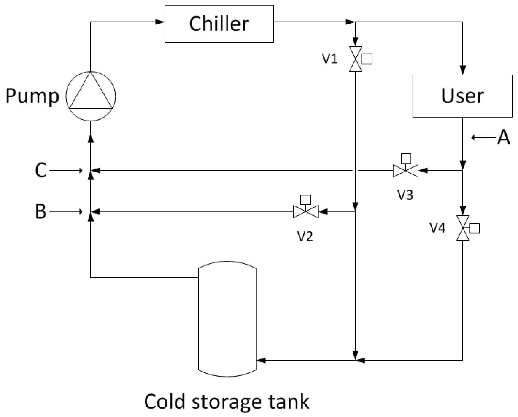
Figure 3 shows a schematic of the layout of the refrigeration system adopted for the implementation of the operational approach described in the previous section.
During chiller operation, the mass flow rate of the heat transfer fluid (HTF) through the user is controlled by means of valve V1 so that the temperature at the user exit—i.e., at point A—is equal to Tc,in. In case the valve V1 is partially open, the HTF passing through V1 goes to the cold storage tank charging it. A further control is applied by means of valve V2 in order to maintain the temperature at point B equal to Tc,in. In this case the valve V3 is fully open while valve V4 is fully close.
Otherwise, in case valve V1 is fully close, which implies that all HTF from the chiller goes to the user and that the HTF exits the user at a temperature that is higher than Tc,in, the cold storage tank is discharged. In this case, a control is applied by means of valve V3 in order to maintain the HTF temperature at point C equal to Tc,in, and also V2 is fully closed.
Assumptions 1 and 2 of the operational approach imply that the mass flow rate of HTF flowing through the user has to be higher than or equal to a minimum value, fixed equal to half the nominal HTF mass flow rate through the chiller, otherwise the chiller is shut down.
3.2. Cold Water Storage Tank Model
1D analytical models have been used in order to simulate the cold water storage tank and the coiled tube heat exchanger [12]. Figure 4 shows a sketch of the close vertical cylindrical tank with a single immersed serpentine considered in the present study. This cold water storage tank configuration, in which the HTF is separated from the water in the tank, permits the use of HTFs different from water, and consequently allows HTF temperatures at the chiller outflow (Tc,out) even slightly higher than 0 °C, as for example 1 °C or 2 °C. Indeed, in such cases it would be not possible to use water as HTF since water could freeze inside the chiller, and a mixture of water and antifreeze should be used.
The internal water volume is divided into isothermal nodes representing water layers of equal volume. The energy balance for each node is written as:
where Qcond represents the conductive heat exchange with adjacent layers. The thermal resistance relative to each layer of the storage wall has been evaluated as:
where
The mean convective heat transfer coefficient relative to the inner tank wall in Equation (3) is evaluated using the Nusselt number correlation for free convection relative to a vertical flat plate [13].
The conductive thermal resistance relative to the tank wall has been evaluated as:
It has been assumed that the tank thickness is equal to the insulation thickness (0.1 m, expanded polyurethane), namely that the conductive thermal resistance of the tank steel wall is negligible.
The convective thermal resistance relative to the external tank wall has been evaluated as:
For each time-step and for each node, the energy balance equations system composed of Equation (1) written for all nodes is solved using the implicit Euler method. The empirical reversion-elimination algorithm [14,15] has been adopted in order to include the effects of natural convection heat transfer between the water layers at different heights on the thermal stratification inside the tank.
A transient one-dimensional model has been adopted for the evaluation of the temperature field of the HTF flowing through the immersed coil heat exchanger. The HTF considered is water.
Also, the heat exchanger has been divided in isothermal nodes representing tube sections having the same volume. For each node, the energy balance equation is given by:
The thermal resistance between the HTF in the coil heat exchanger and the water in the cold storage tank is given by:
where
The mean internal convective heat transfer coefficient in Equation (8) is evaluated using the Gnielinski’s correlation for coiled tube heat exchanger [16] for the Nusselt number calculation.
The external convective thermal resistance has been evaluated as:
The mean external convective heat transfer coefficient in Equation (9) is evaluated using the Morgan’s correlation for natural convection for horizontal cylinders [17] for the Nusselt number.
The conductive thermal resistance of the coil has been neglected, because its order of magnitude is much lower than the internal and external convective thermal resistances.
For each time-step and for each node, Equation (6) is solved using the implicit Euler method.
The coupling between the cold water tank balance equations system and the one relative to the serpentine has been dealt with an iterative approach.
3.3. PCM Storage Tank Model
Figure 5 shows a schematic of the cylindrical cold storage tank with a PCM as storage material considered in this study. The inflow and outflow plenums for the HTF are connected by uniformly distributed straight parallel ¼” pipes passing through the PCM material placed in the central body of the tank, and composing the heat exchanger.
Table 1 reports the main thermo-physical characteristics of the organic PCM considered in the present study. Also in this case, the HTF flowing through the heat exchanger is water.
It has been supposed that the charging and discharging processes are isothermal and realized at the PCM solidification/melting temperature, namely that the cold is stored only as latent heat. Thus, the volume of PCM that is necessary to store a certain amount of cold Ec is given by:
where and are the PCM latent heat of fusion and density, respectively.
The size of the heat exchanger has been evaluated by means of the ε-NTU method [13], implemented on an hourly basis. This method is typically employed for the thermal design of standard heat exchangers, and it has been recently adopted by Tay et al. [18] and Mongibello et al. [19] for latent heat thermal energy storage systems. Therefore, for each pipe of the heat exchanger, the thermal power exchanged between the HTF to the PCM is given by:
where ΔT represents the difference between the HTF temperature at the inlet section of the pipe and the PCM melting temperature, is the mass flow rate of the HTF through the pipe, and ε represents the heat exchanger efficiency, given by:
The number of transfer units NTU is calculated using the following expression:
The overall thermal resistance is given by:
where the thermal resistance relative to the heat transfer between the pipe external surface and the PCM is calculated as:
In Equation (15), the parameter C(δ) refers to the conduction between the pipe external surface and the phase change front supposed concentric to the pipe, and it is a function of the parameter δ representing the ratio between the liquefied portion of the PCM total volume and the PCM total volume. Accordingly, being the phase change front variable with time during the charging phase, the heat exchanger efficiency ε results to be time dependent. Thus, for each operation hour, the average value of the efficiency can be used in Equation (11), that becomes:
For given values of the mass flow rate, of the minutes of operation of the chiller, of the temperature of the HTF entering the storage tank, and of cold to be accumulated at each operation hour, and for a fixed reasonable volume of PCM filling up the storage tank and a fixed aspect ratio of the tank, the number of pipes of the heat exchanger can be evaluated by means of the iterative procedure prescribing the following steps:
- Fix an initial tentative value for the number of pipes;
- Divide the total PCM volume in its initial state by the number of pipes in order to evaluate the volume of PCM surrounding each pipe, that is supposed concentric to the pipe;
- Knowing the cold to be stored or released and the minutes of operation at each hour, evaluate the thermal power to be exchanged at each hour, and evaluate for each hour the fraction of the PCM volume surrounding the pipes that undergoes solidification or melting using Equation (10);
- Knowing the fraction of PCM that has undergone phase change, determine for each hour the average efficiency of the heat exchanger using Equations (12)–(15);
- For each hour, calculate the thermal power exchanged by means Equation (16);
- For each hour, compare the value of thermal power calculated at Step 5 with the one calculated at Step 3. If the maximum of the absolute values of the differences between thermal power values is lower than a certain tolerance, then stop the procedure and accept the number of pipes. Otherwise, increase or reduce the number of pipes as a function of the above differences and return to Step 2.
Finally, once dimensioned the heat exchanger, the energy balance at the heat exchanger pipes permits the calculation of the HTF temperature at the storage tank exit.
The initial tentative value of the number of pipes has to be low enough to avoid the occurrence of conditions in which the cold can be only stored by sensible energy. Indeed, the present model cannot be applied when only sensible energy storage is expected, as for example in the case charging is done when the entire PCM volume is already in the solid phase, or, equivalently, when the discharging is done when the entire PCM volume is already in the liquid one.
A similar procedure can be implemented to evaluate the total PCM volume for a fixed aspect ratio of the tank. In this case, a reasonable number of pipes is fixed, and the total PCM volume is varied in order to match the exchanged thermal power values. Similarly, in this case the initial tentative value of total PCM volume has to be high enough to avoid that the occurrence of conditions in which the cold can be only stored by sensible energy.
4. Results
4.1. Pre-Design
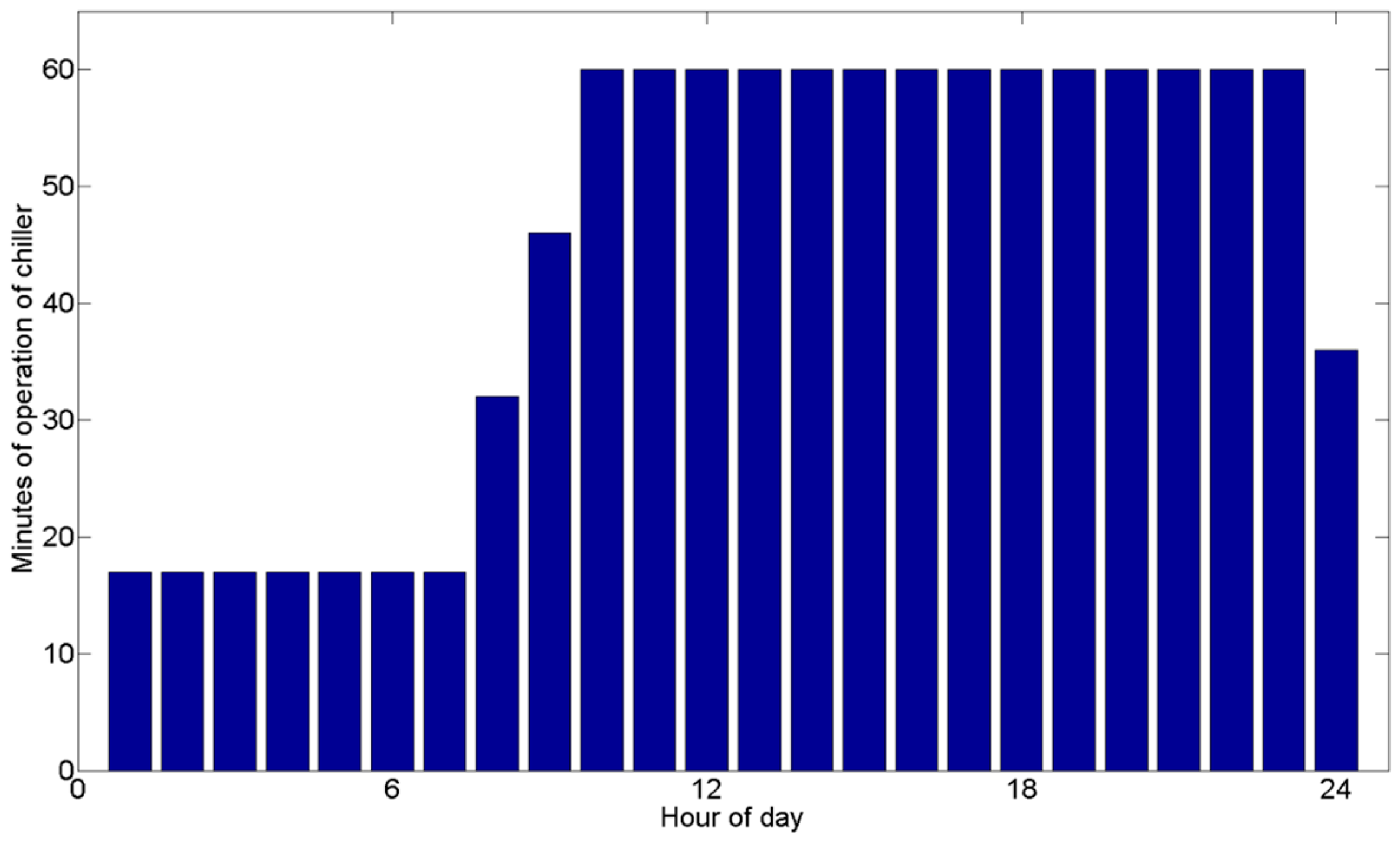
Figure 6 shows the thermal and electrical powers of the chiller through the day, while Figure 7 shows on the same graph the chiller thermal power and the refrigeration loads, resulting from the pre-design. Thus, with the adopted operational approach, the chiller thermal power for the refrigeration system with cold storage resulting from the pre-design is equal to 2.55 kW, with a maximum absorbed electric power of 1.05 kW, that is about the half of the maximum electric power that is needed in the case without the cold storage. Furthermore, it can be noticed the peak-shaving effect due to the cold storage. Figure 8 shows, for each hour of the day, the minutes of operation of the chiller resulting from the pre-design. It can be noticed that, owing to the adopted operational approach, the chiller operation is continuous over a great part of the day, and that the chiller production still remains concentrated in the on-peak hours.
Figure 9 shows, for each hour of the day, the difference between the chiller thermal production and the refrigeration load. The total amount of cold to be stored resulting from the pre-design is 8.4 kWh, that is about the 18% of the user daily total request.
4.2. Cold Water Storage Tank
The numerical simulation of the cold water storage tank has been done assuming that the HTF exits the chiller at a constant temperature Tc,out = 7.0 °C, and at a constant total mass flowrate of 0.1 kg/s. The assumption of constant chiller thermal power implies that the expected temperature of the HTF at the inflow section of the chiller is equal to Tc,in = 13.1 °C.
The volume of the cold water storage tank has been calculated by using the difference between the HTF temperatures at the chiller inflow and outflow sections, namely 13.1 °C and 7 °C, respectively. It is given by:
where SC represents the maximum storage capacity resulting from the pre-design, i.e., 8.4 kWh (30.27 MJ). The resulting water volume is equal to about 1200 L. Finally, a commercial cylindrical tank with a capacitance of 1000 L has been used for the simulations. The tank height from its bottom surface is equal to 2 m (not including insulation), and the entire external surface of the tank is insulated by means of a 0.1 m layer of rigid expanded polyurethane. The tank is provided with a single 1″ serpentine with a heat exchange surface of 8 m2, and the tank capacitance does not include the volume occupied by the serpentine. The inflow section of the serpentine is placed at 5 cm from the tank bottom surface, while the outflow one at 5 cm from the tank top surface. The results of the numerical simulation presented in this section refer to a spatial discretization of the tank realized using 50 nodes, while the serpentine discretization has been made so that its nodes represent the serpentine portions included in the tank layers relative to the tank nodes, and a time-step of 60 s has been adopted. Independence of results from the spatial discretization and time-step has been assured.
The main outputs of the Matlab code are the temperatures at the tank and serpentine nodes. At each time-step, the HTF mass flow rate flowing through the tank heat exchanger, and the HTF temperature at the inflow section of the heat exchanger have been evaluated according to the operation strategy reported in Section 3.1. At each hour, the chiller is active, and the mass flow rate is different from zero, only during the corresponding minutes of operation of the chiller reported in Figure 8. Finally, the following results refer to periodic conditions, obtained starting from an initial temperature of the tank water and of the HTF in the serpentine equal to 13.1 °C.
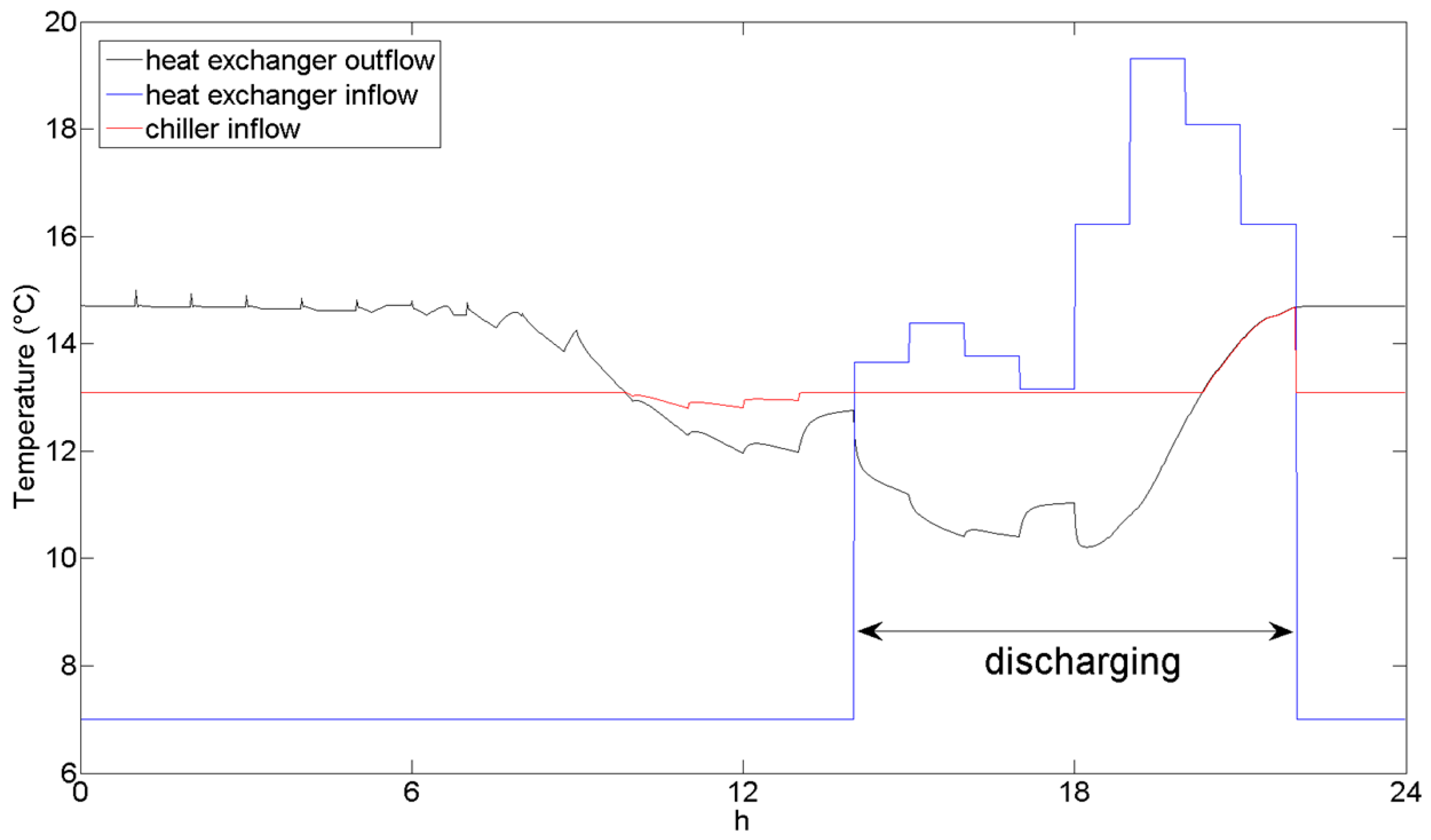
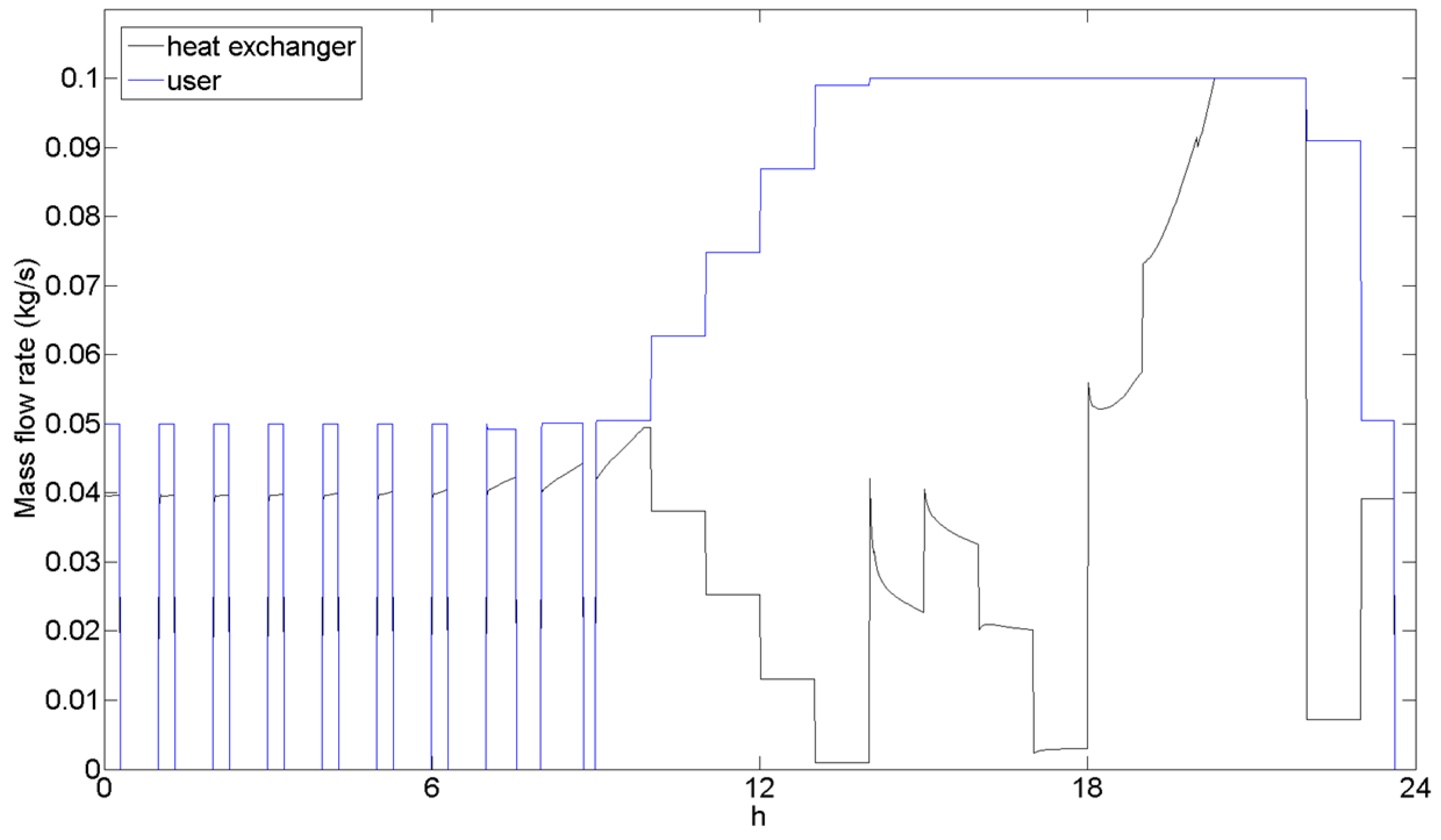
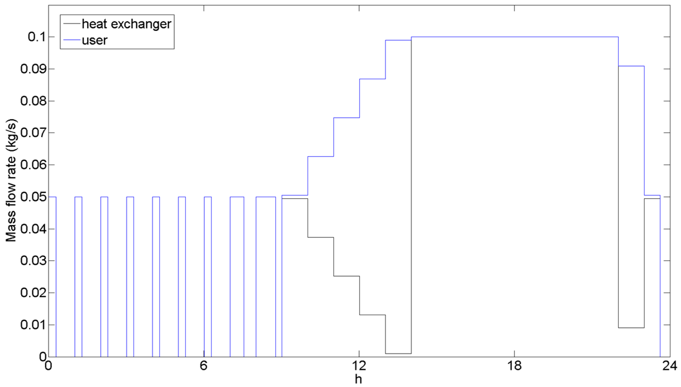
Figure 10 shows the temporal evolution of the HTF temperature at the serpentine outflow during the day, of the HTF temperature at the serpentine inflow, and the resulting temporal evolution of the HTF temperature at the chiller inflow, while Figure 11 shows the HTF mass flow rate through the serpentine and through the user. With reference to Figure 10, it can be noticed that, around h = 12, the HTF temperature at the chiller inflow is slightly lower than the expected value of Tc,in, i.e., 13.1 °C. This is because, in that time interval, the HTF temperature at the serpentine outflow is lower than 13.1 °C, implying that the chiller has to work at a lower power in that period in order to maintain the HTF temperature at its outflow constant and equal to 7 °C.
It can be also noticed that, at the end of the discharging phase, the HTF temperature at the serpentine outflow and the one at the chiller inflow are higher than 13.1 °C. In this case, the chiller has to work consuming a higher electrical power, i.e., 1.3 kW, in order to keep the outflow temperature constant and equal to 7 °C, meaning that a chiller operating at a constant absorbed electric power of 1.05 kW together with the considered cold storage tank is not capable of fulfilling the user request.
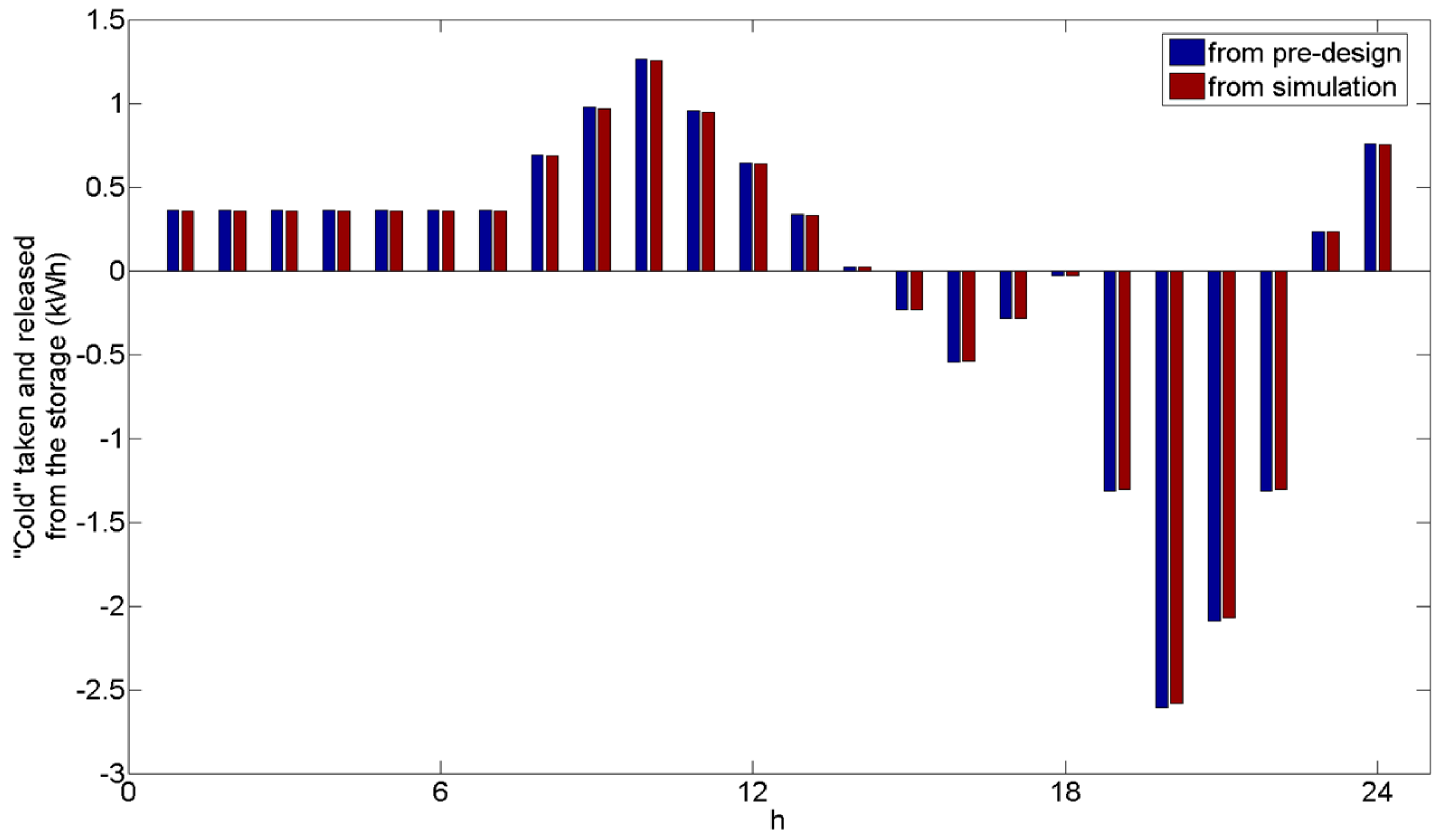
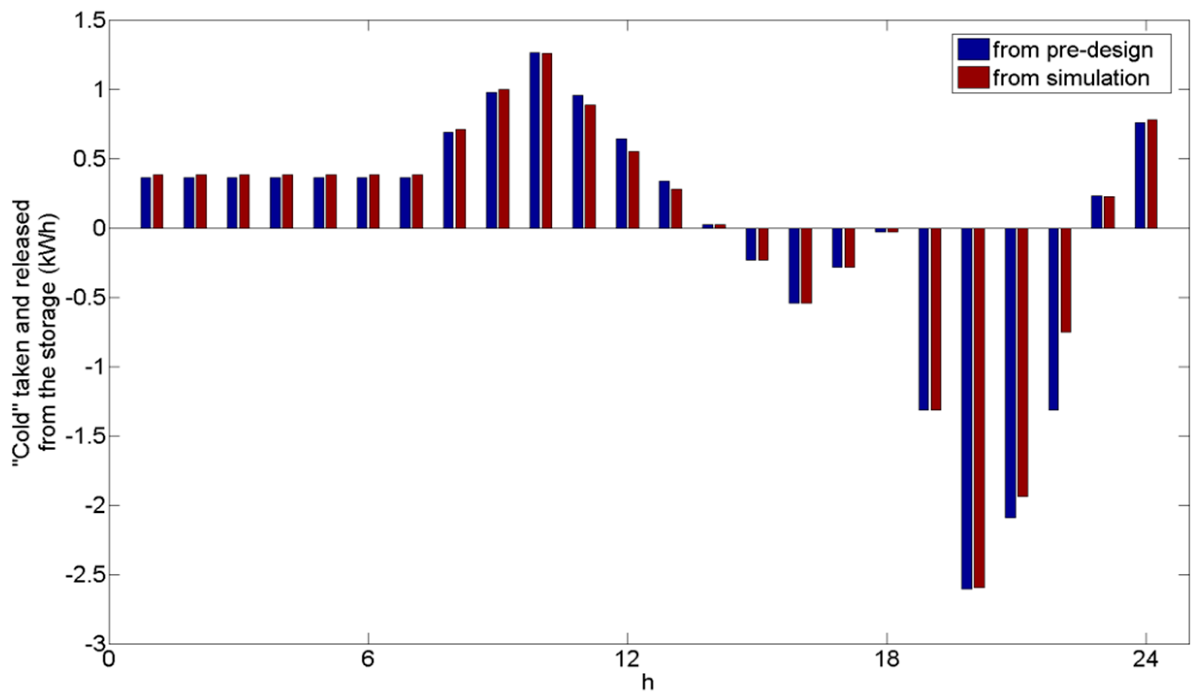
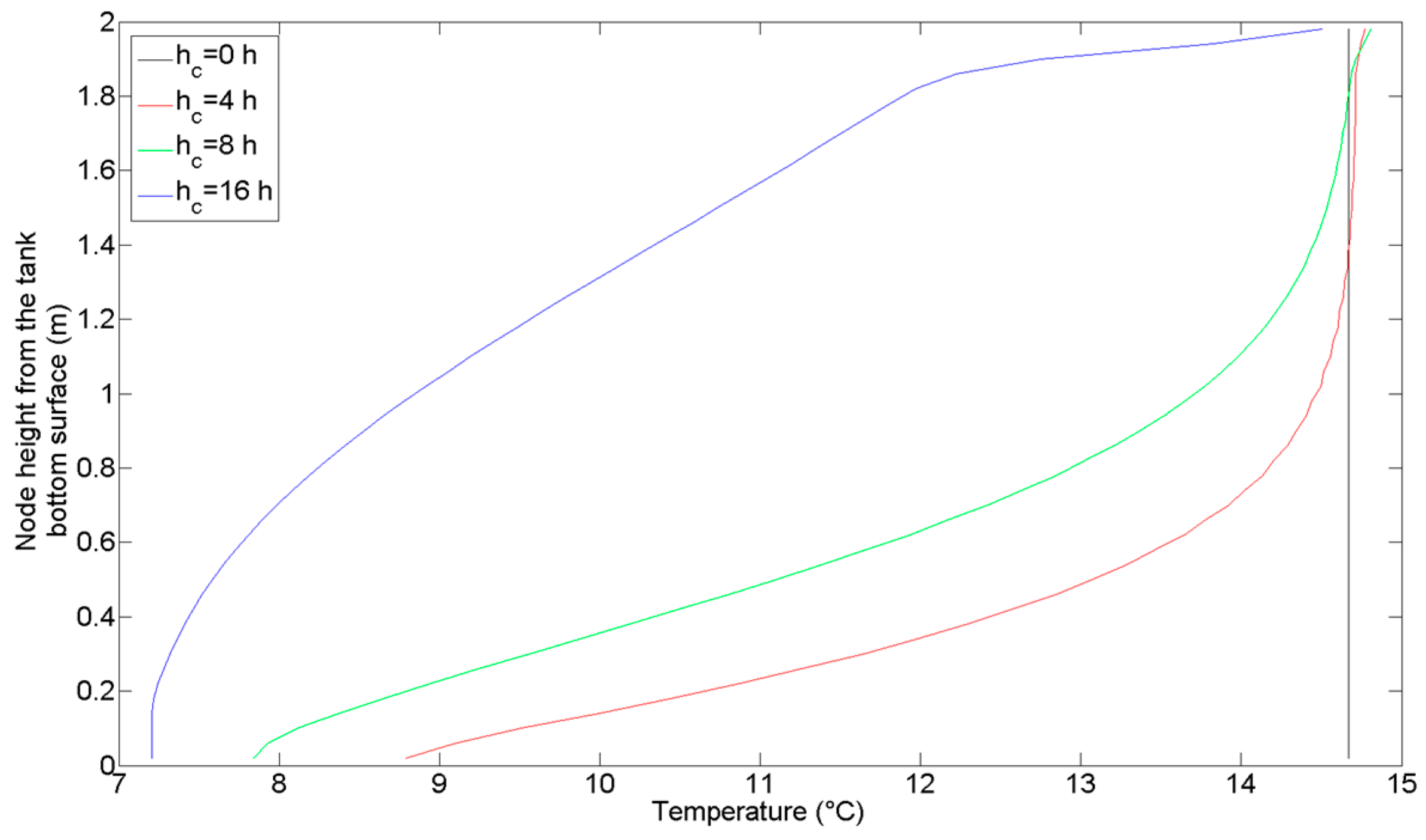
The above considerations are evident if Figure 12, showing the cold taken and released from the storage during the day evaluated in the pre-design, and the ones resulting from the numerical simulations, is analyzed. In fact, it can be seen that, at 11, 12, and 13 h, from the simulation it has emerged that the storage system accumulates less cold than the one resulting from the pre-design. Moreover, it can be seen that at the end of the discharging phase, the cold released by the storage system is much lower than the one evaluated in the pre-design. The reasons explaining the above results are represented by the storage degradation due to the losses through the tank external walls, and to the degradation of the temperature stratification inside the tank. Figure 13 and Figure 14 show the evolution of the water temperature profile in the tank during the charging phase and the discharging one, respectively.
Thus, considering the operation strategy and the size of the cold storage system adopted in this study, in the case with cold storage it is necessary to have a chiller, provided with an inverter, characterized by a maximum absorbed electric power of 1.3 kW, that, however, is much lower than the one in the case without cold storage, namely 2 kW.
From the economic point of view, the chiller and storage tank costs have been evaluated on the basis of real prices in the Italian market. The market price of vapor compression chillers with hydronic loop clearly depends on the chiller size, with the minimum size present in the market equal to 2 kWe at a cost that can be assumed equal to 2500 €. The chiller size in the case with cold storage, i.e., 1.3 kWe, is lower than the above minimum available size in commerce, so its cost has been extrapolated considering an average unitary cost of such chillers in the range from 2 to 10 kWe equal to 800 €/kWe. Hence, as the difference between the chiller absorbed power in the two cases is equal to 700 W, the cost difference is 560 €. Relatively to the storage system cost, considering that it is a closed system not used to store domestic water, its cost can be assumed equal to 1000 €. All the other investment costs have been considered equal in the two different cases.
As concerns the electricity consumption, it is practically the same in the two cases, and this is explained considering that, in the case with cold storage, the consumption surplus due to the higher power needed at the end of the discharging phase is compensated by the higher electricity consumption during night-time at a higher EER. Moreover, in the case without cold storage, it would be necessary to have an available maximum electric power higher than 3 kW in order to avoid power outages during on-peak hours. This would involve an annual fixed cost of 150 €, that is avoided in the case with cold storage.
So, for the present application, the installation of a hydronic vapor compression chiller with cold storage would involve an investment cost that is 440 € higher than the one in the case without cold storage. Nevertheless, due to the avoided annual fixed cost of 150 €, in the case with cold storage the higher investment cost would be returned in less than four years if an interest rate of 5% is applied.
4.3. PCM Storage Tank
Also in this case, it is assumed that the HTF exits the chiller at a constant temperature Tc,out = 7.0 °C, and at a constant total mass flowrate of 0.1 kg/s, and the evaluation of the HTF mass flow rate flowing through the tank heat exchanger and of the HTF temperature at the inflow section of the heat exchanger has been made according to the operation strategy reported in Section 3.1.
The volume of the PCM storage tank has been calculated by means of Equation (10), considering the total amount of cold to be stored equal to the value resulting from the pre-design. The resulting tank volume is 190 L including about 170 kg of PCM. The size of the heat exchanger, considered composed of uniformly distributed straight parallel ¼” pipes, has been calculated following the iterative procedure described in Section 3.3. In particular, the total heat exchange surface has been calculating by fixing the tank aspect ratio at 4, the initial tentative value equal to 2 m2, and a stop condition prescribing that the iterations stop when the maximum normalized difference between the thermal power values from the pre-design and the ones calculated using the model described in Section 3.3 is lower than 1%. The resulting total heat exchange surface is 3.8 m2.
Figure 15 shows the temporal evolution of the HTF temperatures at the pipes inflow and outflow, and the resulting temporal evolution of the HTF temperature at the chiller inflow, while Figure 16 shows the HTF total mass flow rate through the heat exchanger pipes and through the user. It can be seen in Figure 16 that the two profiles are superimposed for 0–9 h in the charging phase, and for 15–22 h during the discharging phase, namely over the entire discharging phase. This last finding indicates that, during discharge, the entire HTF mass flow rate is sent to the cold storage for pre-cooling, and is consistent with the fact that the HTF temperature at the chiller inflow coincide with the one at the heat exchanger outflow over the entire discharging phase, as shown in Figure 15. Figure 15 also shows that the HTF temperature at the chiller inflow is always equal to about 13.1 °C, that is the value of Tc,in from the pre-design, implying that the chiller practically works at constant power during both charging and discharging. Thus, in this case, the chiller operating at a constant absorbed electric power of 1.05 kW—i.e., the absorbed power resulting from the pre-design—together with the considered PCM storage tank are able to fulfill the user request. This result is confirmed by Figure 17, showing that the profile of the cold taken and released from the storage during the day evaluated by means of the PCM storage tank model is practically the same as the one resulting from the pre-design.
However, as regards the economic aspects, the estimated cost of the PCM (8 €/kg) and the one of the non-standard tank (around 500 €) make this solution impractical from the economic point of view. In this case, about the same payback period as in the case with cold water storage can be obtained with a target cost for the PCM of 3 €/kg.
5. Conclusions
In this work, the operation, modeling, simulation, and cost evaluation of two different cold storage systems for a single-family house in Italy, that differ from one another on the cold storage material, have been addressed. The two materials used to perform the numerical simulations of the cold storage systems are represented by cold water and a phase change material, and the numerical simulations have been realized by means of numerical codes written in Matlab environment.
Results have shown that, for the considered user characteristics, a cold water storage system characterized by an effective operation strategy could represent a viable solution from the economical point of view.
Future studies may regard the dimensioning of a storage system integrated into the fluidic system of a reversible vapor compression heat pump, that can be also used to store heat during the cold season.
Author Contributions
Both authors conceived the work. Luigi Mongibello selected the models and realized the numerical codes for the simulations. Both authors analyzed the data resulting from the numerical simulations. The paper was written by Luigi Mongibello, and revised by both authors.
Conflicts of Interest
The authors declare no conflict of interest.
References
- Silvetti, B.; MacCracken, M. Thermal storage and deregulation. ASHRAE J. 1998, 4, 55–59. [Google Scholar]
- Wang, S.K. Handbook of Air Conditioning and Refrigeration, 2nd ed.; McGraw-Hill: New York, NY, USA, 2001. [Google Scholar]
- Lin, H.; Li, X.H.; Cheng, P.S.; Xu, B.G. Thermoeconomic evaluation of air conditioning system with chilled water storage. Energy Convers. Manag. 2014, 85, 328–332. [Google Scholar] [CrossRef]
- Yan, C.; Shi, W.; Li, X.; Zhao, Y. Optimal design and application of a compound cold storage system combining seasonal ice storage and chilled water storage. Appl. Energy 2016, 171, 1–11. [Google Scholar] [CrossRef]
- Soler, M.S.; Sabaté, C.C.; Santiago, V.B.; Jabbari, F. Optimizing performance of a bank of chillers with thermal energy storage. Appl. Energy 2016, 172, 275–285. [Google Scholar] [CrossRef]
- Kintner-Meyer, M.; Emery, A. Optimal control of an HVAC system using cold storage and building thermal capacitance. Energy Build. 1995, 23, 19–31. [Google Scholar] [CrossRef]
- Habeebullah, B.A. Economic feasibility of thermal energy storage systems. Energy Build. 2007, 39, 355–363. [Google Scholar] [CrossRef]
- Sun, Y.; Wang, S.; Xiao, F.; Gao, D. Peak load shifting using different cold thermal energy storage facilities in commercial buildings: A review. Energy Convers. Manag. 2013, 71, 101–114. [Google Scholar] [CrossRef]
- Navidbakhsh, M.; Shirazi, A.; Sanaye, S. Four E analysis and multi-objective optimization of an ice storage system incorporating PCM as the partial cold storage for air-conditioning applications. Appl. Therm. Eng. 2013, 58, 30–41. [Google Scholar] [CrossRef]
- Oró, E.; Depoorter, V.; Plugradt, N.S.J. Overview of direct air free cooling and thermal energy storage potential energy savings in data centres. Appl. Therm. Eng. 2015, 85, 100–110. [Google Scholar] [CrossRef]
- Mongibello, L.; Bianco, N.; Caliano, M.; Graditi, G. Influence of heat dumping on the operation of residential micro-CHP system. Appl. Energy 2015, 160, 206–220. [Google Scholar] [CrossRef]
- Mongibello, L.; Bianco, N.; Caliano, M.; de Luca, A.; Graditi, G. Transient analysis of a solar domestic hot water system using two different solvers. Energy Procedia 2015, 81, 89–99. [Google Scholar] [CrossRef]
- Bejan, A.; Kraus, A.D. Heat Transfer Handbook; John Wiley & Sons Inc.: Hoboken, NJ, USA, 2003. [Google Scholar]
- Mather, D.W.; Hollands, K.G.T.; Wright, J.L. Single- and Multi-Tank energy storage for solar heating systems: Fundamentals. Sol. Energy 2002, 73, 3–13. [Google Scholar] [CrossRef]
- Newton, B.J.; Schmid, M.; Mitchell, J.W.; Beckman, W.A. Storage tank models. In Proceedings of the ASME/JSME/JSES International Solar Energy Conference, Maui, HI, USA, 19–24 March 1995.
- Gnielinski, Y. Heat transfer and pressure drop in helically coiled tubes. In Proceedings of the 8th International Heat Transfer Conference, San Francisco, CA, USA, 17–22 August 1986; Volume 6, pp. 2847–2854.
- Morgan, V.T. The overall convective heat transfer from smooth circular cylinders. Adv. Heat Transf. 1975, 11, 199–264. [Google Scholar]
- Tay, N.H.S.; Belusko, M.; Bruno, F. An effectiveness-NTU technique for characterising tube-in-tank phase change thermal energy storage systems. Appl. Energy 2012, 91, 309–319. [Google Scholar] [CrossRef]
- Mongibello, L.; Capezzuto, M.; Graditi, G. Technical and cost analyses of two different heat storage systems for residential micro-CHP plants. Appl. Therm. Eng. 2014, 71, 636–642. [Google Scholar] [CrossRef]
Figure 1.
Refrigeration loads of the user.
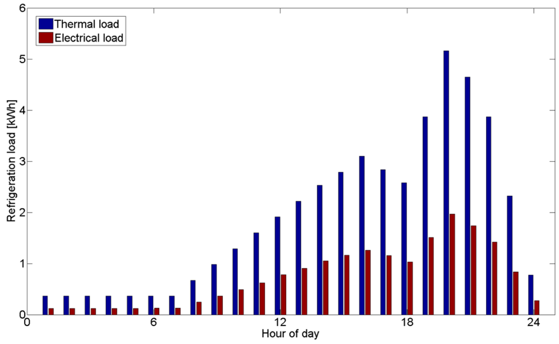
Figure 2.
Non-dimensional temperature and EER profiles.
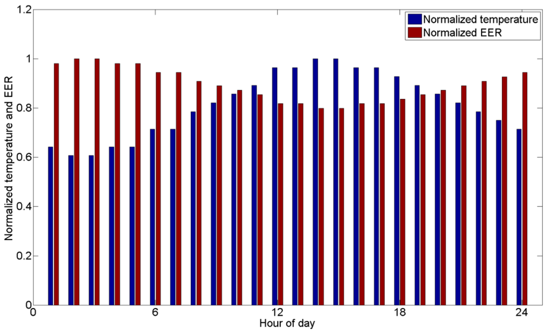
Figure 3.
Layout of the refrigeration system.

Figure 4.
Sketch of the cold water storage tank.
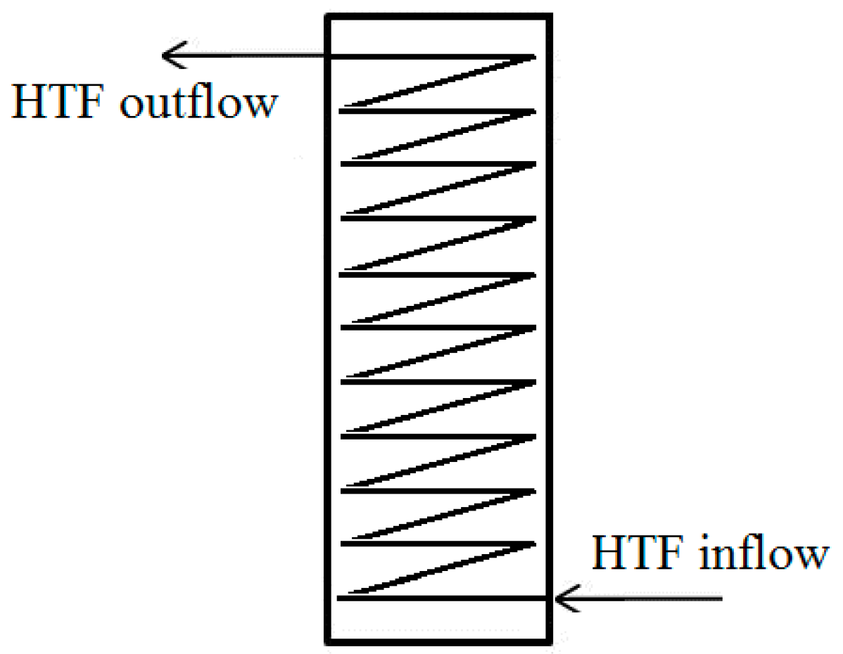
Figure 5.
Schematic of the cold storage tank with PCM.
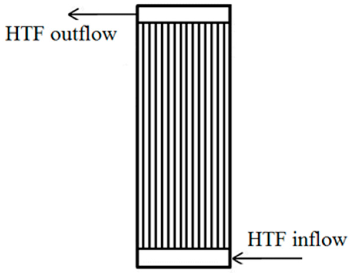
Figure 6.
Chiller power with cold storage.
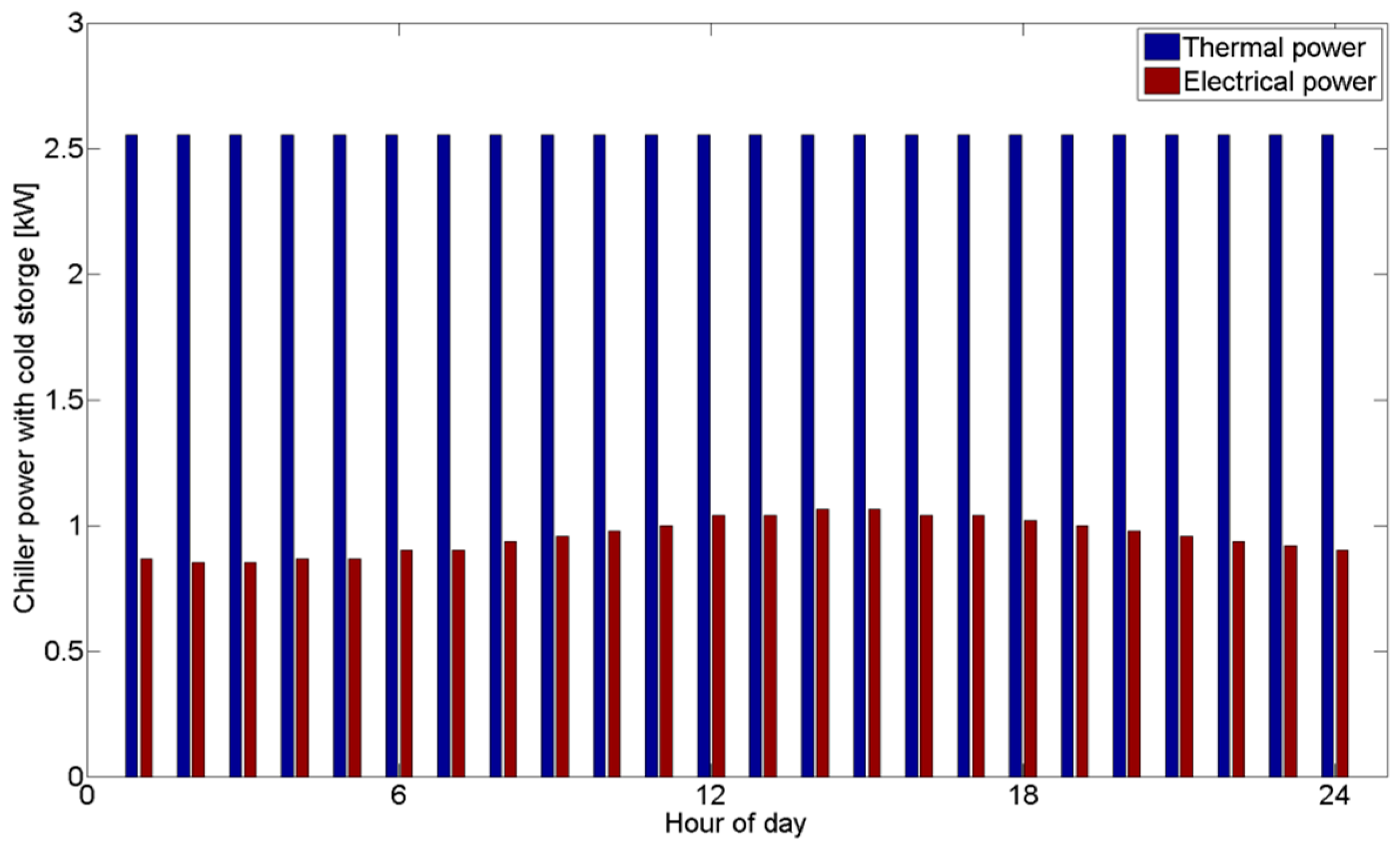
Figure 7.
Chiller thermal power and refrigeration loads.
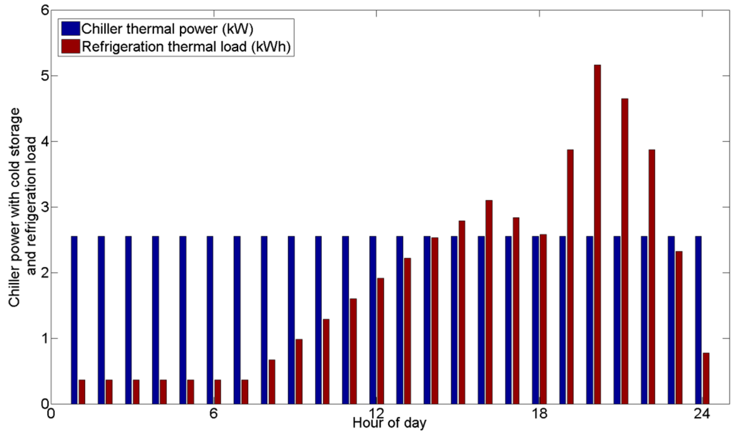
Figure 8.
Minutes of operation of the chiller.

Figure 9.
Difference between the chiller thermal production and the refrigeration loads.
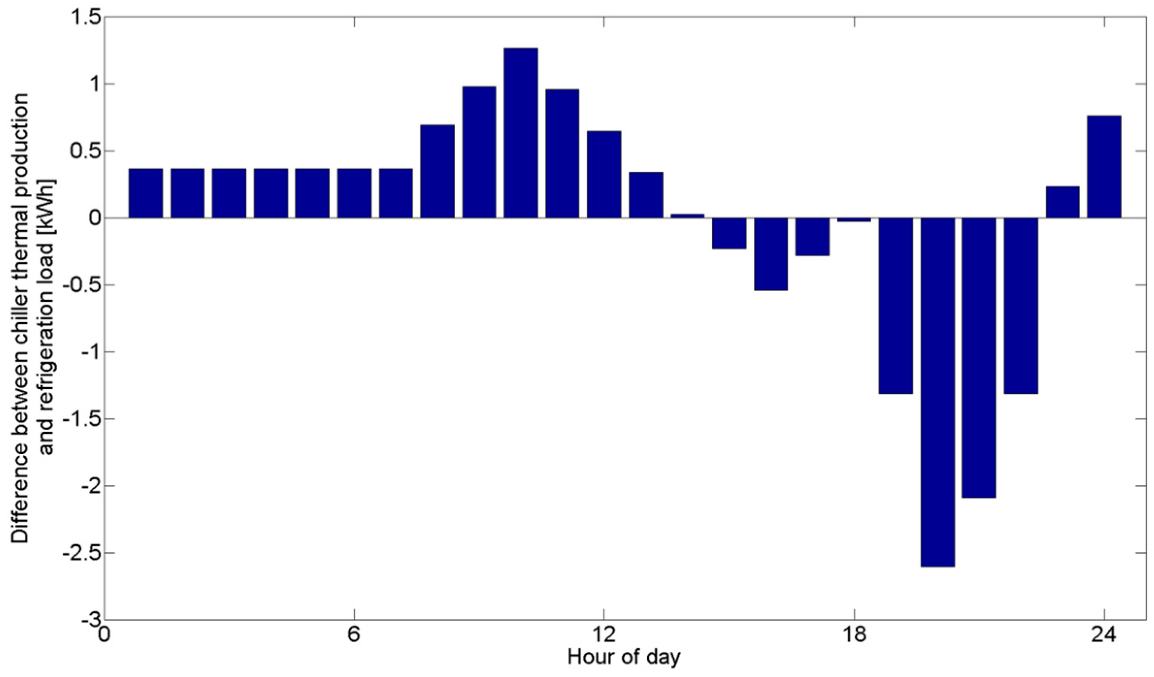
Figure 10.
HTF temperature profiles at the water tank heat exchanger inflow and outflow sections, and at the chiller inflow section.
Figure 10.
HTF temperature profiles at the water tank heat exchanger inflow and outflow sections, and at the chiller inflow section.

Figure 11.
HTF mass flow rate through the water tank heat exchanger and the user.

Figure 12.
“Cold” taken and released from the cold water tank.

Figure 13.
Temperature profiles in the cold water tank during the charging phase (hc = 0 h refers to the beginning of the phase).
Figure 13.
Temperature profiles in the cold water tank during the charging phase (hc = 0 h refers to the beginning of the phase).

Figure 14.
Temperature profiles in the cold water tank during the discharging phase (hd = 0 h refers to the beginning of the phase).
Figure 14.
Temperature profiles in the cold water tank during the discharging phase (hd = 0 h refers to the beginning of the phase).
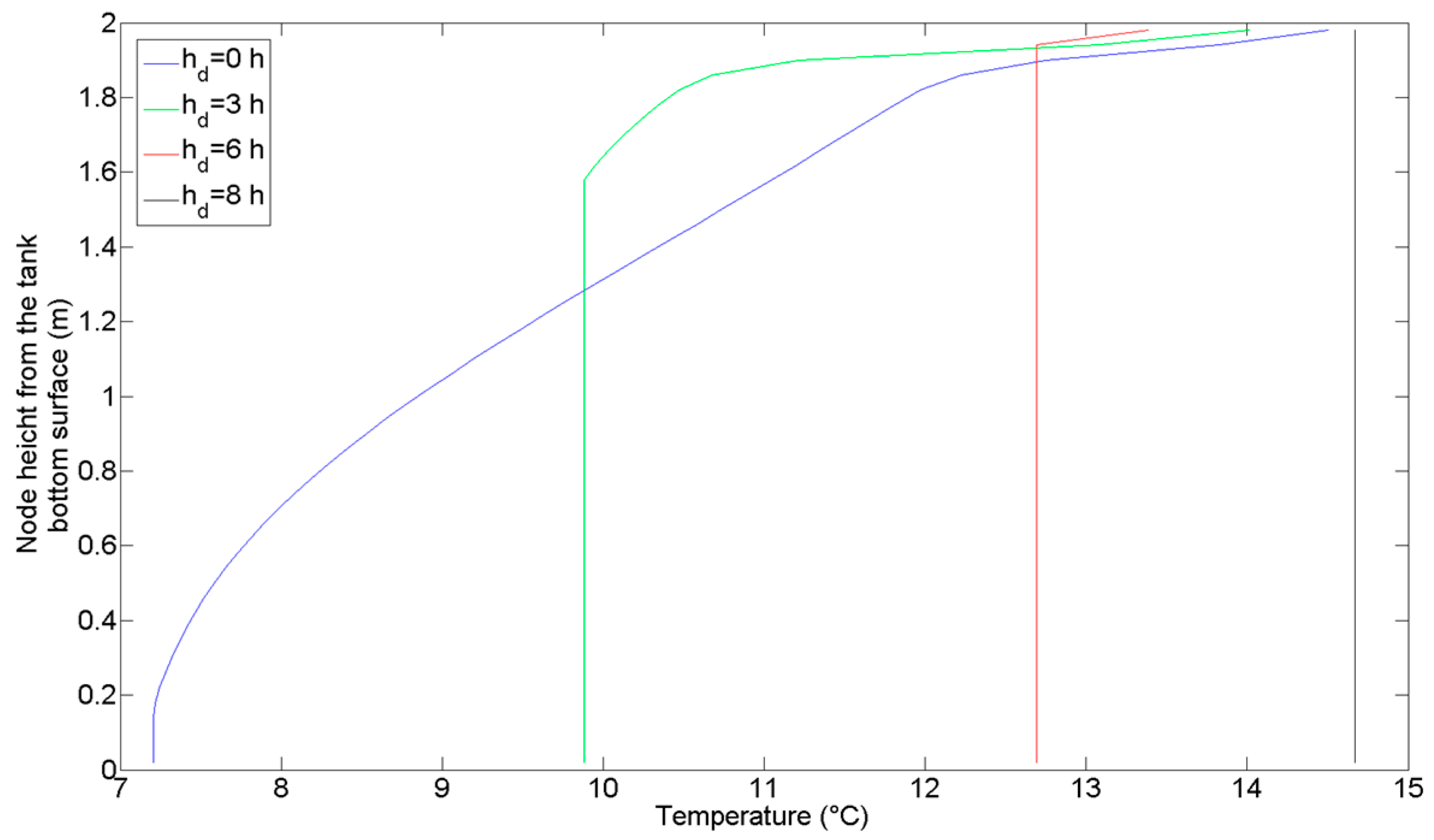
Figure 15.
HTF temperature profiles at the PCM tank heat exchanger inflow and outflow sections, and at the chiller inflow section.
Figure 15.
HTF temperature profiles at the PCM tank heat exchanger inflow and outflow sections, and at the chiller inflow section.
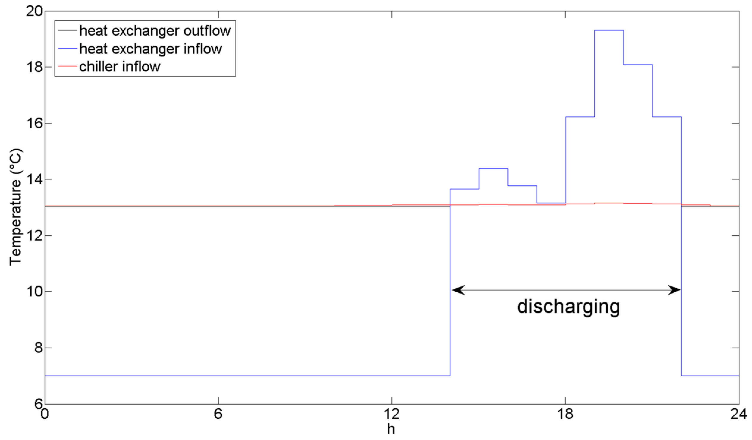
Figure 16.
HTF mass flow rate through the PCM tank heat exchanger and the user.

Figure 17.
“Cold” taken and released from the PCM tank.

| Property | Value |
|---|---|
| Density | 900 kg/m3 |
| Thermal conductivity | 0.2 W/m/K |
| Latent heat of fusion | 18 × 104 J/kg |
| Melting temperature | 13 °C |
© 2016 by the authors; licensee MDPI, Basel, Switzerland. This article is an open access article distributed under the terms and conditions of the Creative Commons Attribution (CC-BY) license (http://creativecommons.org/licenses/by/4.0/).
Share and Cite
MDPI and ACS Style
Mongibello, L.; Graditi, G. Cold Storage for a Single-Family House in Italy. Energies 2016, 9, 1043. https://doi.org/10.3390/en9121043
AMA Style
Mongibello L, Graditi G. Cold Storage for a Single-Family House in Italy. Energies. 2016; 9(12):1043. https://doi.org/10.3390/en9121043
Chicago/Turabian StyleMongibello, Luigi, and Giorgio Graditi. 2016. "Cold Storage for a Single-Family House in Italy" Energies 9, no. 12: 1043. https://doi.org/10.3390/en9121043
Note that from the first issue of 2016, this journal uses article numbers instead of page numbers. See further details here.