Article

Structural Dynamic Analysis of Semi-Submersible Floating Vertical Axis Wind Turbines

1
Department of Mechanical and Structural Engineering and Material Science, University of Stavanger, 4036 Stavanger, Norway
2
Aker Solutions AS, 1366 Lysaker, Norway
*
Author to whom correspondence should be addressed.
Energies 2016, 9(12), 1047; https://doi.org/10.3390/en9121047
Submission received: 5 August 2016 / Revised: 3 October 2016 / Accepted: 5 December 2016 / Published: 13 December 2016
(This article belongs to the Special Issue Modeling and Simulation for Wind Turbine Loads Analysis)

Abstract

:
The strong and stable wind at offshore locations and the increasing demand for energy have made the application of wind turbines in deeper water surge. A novel concept of a 5 MW baseline Floating Vertical Axis Wind Turbine (FVAWT) and a 5 MW optimised FVAWT with the DeepWind Darrieus rotor and the optimised DeepWind Darrieus rotor, respectively, were studied extensively. The structural responses, fatigue damages, platform global motions and mooring line dynamics of the FVAWTs were investigated comprehensively during normal operating conditions under steady wind and turbulent wind conditions, using a coupled non-linear aero-hydro-servo-elastic code (the Simo-Riflex-DMS code) which was developed by Wang et al. for modeling FVAWTs. This coupled code incorporates the models for the turbulent wind field, aerodynamics, hydrodynamics, structural dynamics, and generator controller. The simulation is performed in a fully coupled manner in time domain. The comparison of responses under different wind conditions were used to demonstrate the effect of turbulence on both FVAWTs dynamic responses. The turbulent wind condition has the advantage of reducing the 2P effects. Furthermore, comparative studies of the FVAWTs responses were undertaken to explore the advantages of adopting the optimised 5 MW DeepWind Darrieus rotor over the baseline model. The results identified the 5 MW optimised FVAWT to having: lower Fore-Aft (FA) but higher lower Side-Side (SS) bending moments of structural components; lower motions amplitude; lower short-term fatigue equivalent loads and a further reduced 2P effects.

1. Introduction

The risk, price inconsistency and environmental impact associated with oil and gas exploration and production have driven a focus on renewable energy. Wind power, the fastest growing source of renewable power generation in Europe, is a major competitor to oil and gas. The strong and stable wind at offshore locations and the increasing demand for energy have surged the application of wind turbines in deep water.
The Floating Horizontal Axis Wind Turbine (FHAWT) has been a research focus in deep water wind power production due to its commercial success in onshore applications. However, the application of Floating Vertical Axis Wind Turbines (FVAWT) in deep offshore waters has potential because of their economic advantages in installation and maintenance. The application of Vertical Axis Wind Turbines (VAWT) rotor technology in large wind turbines could reduce the cost-of-energy (COE) by over 20% [1]. Furthermore, due to the higher maintainability of FVAWTs, their ability to capture wind energy irrespective of wind direction without a yaw control mechanism, lower center of gravity, economies of installation amongst other designs as compared with FHAWTs [2], FVAWTs could be a better concept in deeper water applications. These aforementioned advantages have steered resurgence of interest in research on the application of FVAWTs in deep waters [3,4]. Studies have focused on the design, structural integrity, dynamic response and installation methodologies to better understand the performance of the various concepts and to provide the basis for detailed structural designs [5,6,7,8,9,10]. Hence, various concepts were developed and investigated for use as floating substructures to support wind turbines. These concepts include the spar [11], the semi-submersibles [7,10] and the Tension Leg Platform (TLP) concept [12].
The dynamic response of a floating wind turbine differs significantly from that of a bottom-supported substructure or a land-based wind turbine. Floating wind turbines will experience large aerodynamic and hydrodynamic loads, including loads due to the rotating blades. Therefore, it is pertinent to analyze numerous substructure concepts in order to understand their respective responses and suitability for a particular sea state. Various FVAWT concepts have been evaluated, such as the DeepWind concept [13,14,15], the VertiWind concept [16] and the Aerogenerator X concept [17], for conceptual designs and technical feasibility. The DeepWind concept and the VertiWind concept were studied, but the AeroGenerator-X concept was only proposed without any detailed report or relevant publication. A novel concept combining the DeepWind 5 MW rotor [18] and the DeepCwind floater from the Offshore Code Comparison Collaboration Continuation (OC4) project [19], were extensively investigated as well. Furthermore, a variety of studies applied different simulation tools to investigate the response characteristics of FVAWTs to provide the conceptual design descriptions and detailed evaluation of technical feasibilities of the various concepts.
Limited state-of-art simulation codes have been developed over the years for conceptual evaluation of FVAWTs. These include (Horizontal Axis Wind turbine simulation Code 2nd generation) HAWC2, (Floating Vertical Axis Wind Turbine) FloVAWT, Simo-Riflex-DMS, etc. HAWC2 [20,21,22] was developed at Risø, Technical University of Denmark (DTU). In order to equip HAWC2 with the ability to model FVAWTs in the time domain for the DeepWind FVAWT an improved aero-elastic code based on the Actuator Cylinder (AC) model was linked to it using a Dynamic Link Library (DLL). HAWC2 is a multi-body simulation tool which allows the separate modelling of individual components of a turbine. However, the hydrodynamic model employed is more accurate for slender substructures like spars (Morrison-like structures), thus, it is considered unsuitable for analysing structures such as semi-submersibles. The coupled aero-hydro-servo-elastic code, Simo-Riflex-Aerodyn was also developed [23] to fully integrate the complete features of Aerodyn [24] into Simo-Riflex coupled code. However, this is used for modeling FHAWT and is not suitable for FVAWT. At Cranfield University in the UK, Borg et al. [25] developed a simplified coupled code designed using MATLAB programming for preliminary design analysis of FVAWTs. This code is called FloVAWT. The code has been in continual development and verification by Collu et al. [26]. However, the code was criticized for lacking a structural model, mooring line model and dynamic control model, hence, a rigid rotor is assumed to rotate at constant speed while the relationship between force-displacement is linearized. A non-linear aero-hydro-servo-elastic, Simo-Riflex-DMS was developed by Wang et al. [27] for modeling FVAWTs with semi-submersible substructure. The Double Multiple Streamtube (DMS) code [
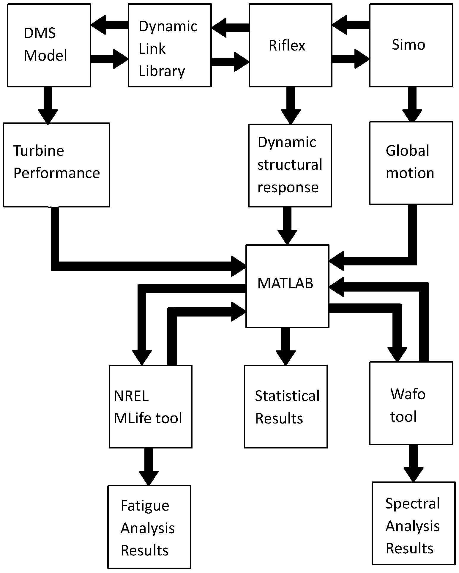
28] is an aero-elastic code used to model the aerodynamic loads on the wind turbine rotor. The Riflex code is the finite element solver and as well, serve as a link to external modules/codes while the SIMO code is used to model the floater hydrodynamics. Therefore, Simo-Riflex-DMS code coupled the aerodynamic, the hydrodynamic, the structural dynamic and the generator controller modules. The Simo-Riflex-DMS has been used to study a novel concept that combined the DeepWind 5 MW rotor [18] and the DeepCwind floater from the OC4 project [19], in a fully coupled time domain simulation [27]. The Simo-Riflex-DMS model, as developed by Wang et al. [27], is adopted for this work.
The dynamic analysis and comparative studies of different FVAWT concepts have been performed. These include the dynamic analysis of a 5 MW Darrieus curved bladed VAWT with rotating foundation [29]. However, the VAWT was coupled to a spar platform. A further analysis of this concept has been carried out at DTU, to reduce the VAWT’s weight and the bending loads on the rotor [30]. A novel concept that combines the 5 MW Darrieus curved blade VAWT with a semi-submersible platform has been extensively studied by Wang et al. [2,4,31]. Additionally, a comparative study of the FVAWT concept by Wang with two similar FVAWT concepts (a combination of the 5 MW Darrieus curved bladed VAWT with: 1) a spar platform and 2) a TLP, has been performed by Cheng et al. [32]. He concluded that the semi-submersible and the spar abated the 2P effects on structural loads and mooring line tensions as compared to the TLP concept, at the expense of larger platform motions. A further study has been carried out to evaluate the effect of difference-frequency forces on a FVAWT with semi-submersible platform under misaligned wind-wave conditions [33]. The effect of wind-wave misalignment and the second order difference frequency force on the FVAWT were more significant at extreme values of the responses, especially at wind speeds above the rated wind speed.
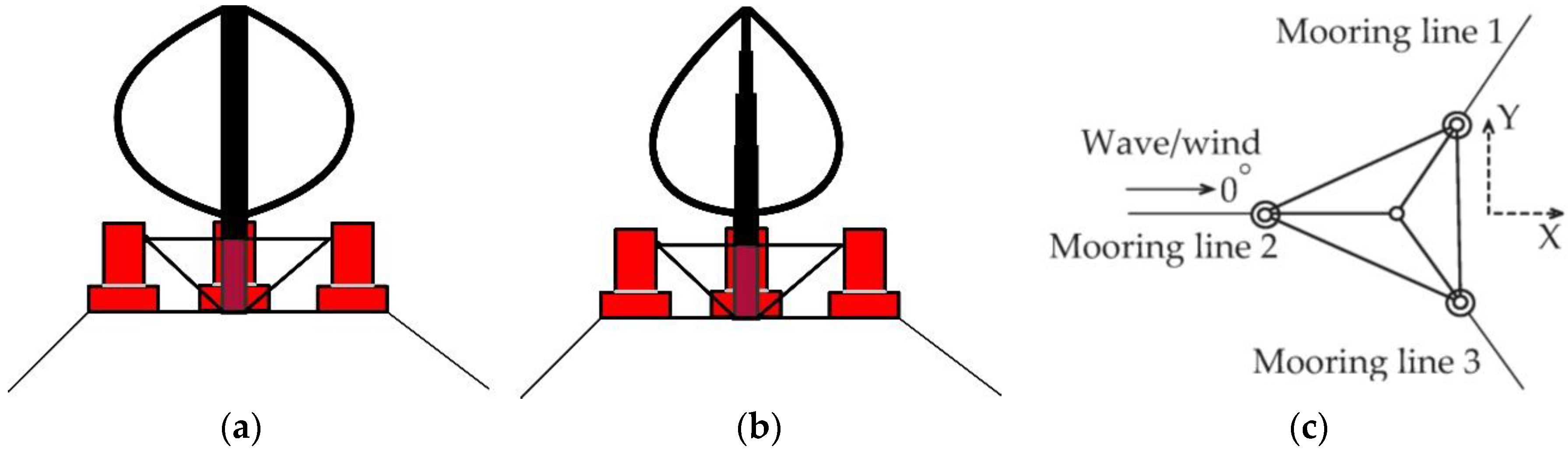
In this work, a baseline semi-submersible FVAWT concept [34] is adopted. This concept has been studied in a systematic manner: a method for the analysis has been developed; global motion for the floating support structure was comprehensively analyzed—considering normal operating condition and emergency shutdown; a comparative analysis between the proposed model and an equivalent model of an Horizontal Axis Wind Turbine (HAWT) rotor has been carried out including a stochastic analysis of the model [2,4,25,27,31,33,35,36]. Furthermore, the response of the concept in combination with an hydrodynamic brake under emergency condition has been investigated [
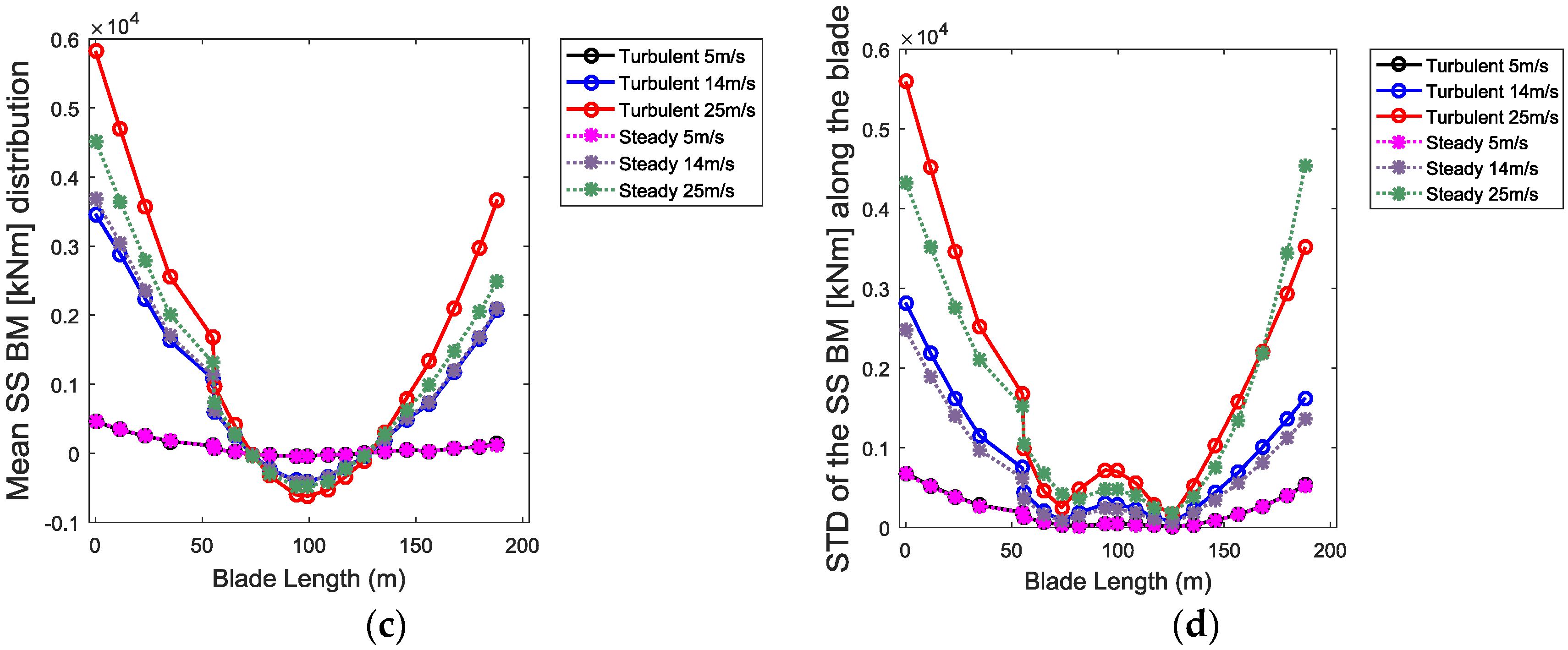
31]. However, extensive investigations of structural responses of flexible components such as the blades, the tower and the mooring lines, include the blade bending moment distributions and fatigue responses have not been carried out. For FVAWTs, the continuously varying aerodynamic loads on the rotor lead to a considerably higher load level and increasing number of load cycles. Therefore, it is significant to evaluate fatigue damage based on the time history of FVAWTs responses. The rainflow counting technique is used for the fatigue cycle counting while the Mlife tool from the National Renewable Energy Laboratory (NREL) is used to calculate the short-term fatigue damage equivalent loads for the FVAWT.
The dynamic responses of the 5 MW baseline FVAWT were investigated by analyzing the platform global motion, the analysis of structural loads of flexible components, and the estimation of the short-term fatigue damage equivalent loads of the structural components. Furthermore, this work is extended to evaluate the performance of a 5 MW optimized FVAWT in terms of power production, structural dynamic response, global motion and short-term fatigue damage on structural components. The 5 MW optimized FVAWT is a concept combining the optimized 5 MW DeepWind rotor [30] from the Technical University of Denmark (DTU) and the DeepCwind semi-submersible from the OC4 project [19]. The 5 MW DeepWind rotor was optimised by a group of researchers at DTU. The tower of the rotor is optimized to weighs 67% less than the tower for the baseline 5 MW DeepWind rotor with lower bending moments [37]. The two FVAWT models were evaluated under the same environmental conditions. A comparative analysis of the response results of both FVAWT models are presented to explore the advantages of the optimized 5 MW DeepWind rotor.

2. Methodology

2.1. The Floating Vertical Axis Wind Turbine Models

This study considers two wind turbine models: a 5 MW baseline FVAWT shown in Figure 1a and a 5 MW optimized FVAWT illustrated in Figure 1b. The 5 MW baseline FVAWT concept is fully described in [34]. The design consists of a semi-submersible substructure [38] with a curved Darrieus VAWT [29], consisting of a generator assumed to be positioned at the tower bottom in the central column of the semi-submersible. The platform global motion is limited by anchoring the semi-submersible to the sea bottom by means of catenary mooring system in Figure 1c. Furthermore, the sea water dampens the platform dynamics. This novel FVAWT concept has been studied by Wang [34].
The 5 MW optimized FVAWT is similar to the 5 MW baseline FVAWT, except the turbine rotor is the 5 MW optimized DeepWind rotor from DTU [30]. The Simo-Riflex-DMS code developed by Wang et al. [27], which has been validated and extensively used by Wang [33,34] and other professionals [32,35], is adopted for the numerical simulations of the FVAWTs.

2.2. A Method for the Platform Adaptation

The 5 MW optimised DeepWind rotor weighs about 41% less than the 5 MW VAWT baseline rotor. Hence, if the optimised DeepWind rotor is to be coupled directly, the original draft of the platform will reduce. This will cause the mooring lines to be pre-tensioned at their undisplaced position because the length of the mooring lines and position of fairleads are unchanged. The idea is to maintain the platform properties. Therefore, the semi-submersible from the DeepCwind phase II of the OC4 Project [19] must be slightly modified to maintain the same draft as the original platform. This is achieved by increasing the mass of ballast water. The following assumption, approximation and notation were applied to successfully modify the platform:
  • The ballast water is sea water with density ρ = 1.025 t/m3.
  • From the platform detailed specifications [19], 25% and 75% of ballast mass were placed in the Upper Column (UC) and Base Column (BC) of offset columns respectively. No ballast in Centre Column CM.
  • At the platform undisplaced position, the ballast mass geometry can be assumed as solid cylinder with mass.
  • The FVAWT is assumed to be symmetrically loaded and thus, the method of buoyancy compensating force [39] is applied in SIMO.
  • The distance from the centre of mass of ballast water to the CM equals the distance from the centre of mass of UC or BC to CM.
To annul the inconsistency between Riflex and SIMO in the interpretation of the body forces in the coupled model, the method of buoyancy compensation force [39] is applied to ensure a correct static configuration. This further reduce the instability that may be associated with running the simulation.
The following methodology is used to modify the platform slightly in order to support the 5 MW optimised FVAWT. Furthermore, this approach can be adapted for similar scenario, where a slight modification of the platform weight is required to maintain the platform draft to support a wind turbine of different weight or a topside. However, some of the steps would need to be applied appropriately to reflect the uniqueness of case under consideration:
  • Calculate the original FVAWT submerged mass. To maintain the same draft, the submerged mass of both the original FVAWT and the modified FVAWT must be equal.
  • Subtract the respective total mass of flexible elements and the total platform metal mass from the submerged masses to obtain the masses of ballast water for the respective FVAWTs.
  • Calculate the mass moment of inertia due to the mass of ballast water about the three axis of rotation taking the third assumption into consideration for both the original and modified platform.
  • Subtract the inertias for the original platform obtained in step 3 from the original total platform inertias and then add the inertias due to mass of ballast of the modified platform obtained in step 3.
The moment of inertias were estimated by applying the basic definition of moment of inertia for a cylindrical object about its centre, considering the assumptions. The empty portion of offset columns were considered as open cylinders while the portions filled with ballast water were considered as solid cylinder. The parallel axis theorem is used to compute the inertias about the platform’s centre of mass (Xg, Yg, Zg). However, the calculated moment of inertias are with respect to the center of gravity of local coordinates. To apply this into the symmetrical structural mass coefficient in the Simo code, they must be transformed to the global coordinate system as described in (1):
RIXX   = I XX +   M B ( Y g 2 +   Z g 2   ) RIYY   = I YY +   M B ( X g 2 +   Z g 2   ) RIZZ   = I ZZ +   M B ( X g 2 +   Y g 2   ) ,
where I and MB are the moment of inertia (with respect to the center of gravity of local coordinates) and the structural mass respectively. For more details, see the Simo manual [40].
The change in platform weight as a result of the change in ballast mass must be accounted for in the calculations of the hydrostatic stiffness data. Hence, the part of the restoring terms C(4, 4), C(5, 5) in the hydrodynamic stiffness data is estimated as given in (2) to obtain the modified C(4, 4)New and C(5, 5)New [41]:
C ( 4 , 4 ) New = C ( 4 , 4 ) M O g Z g O + M P g Z g C ( 5 , 5 ) New = C ( 5 , 5 ) M O g Z g O + M P g Z g ,
where MO and Z g O are the total mass and center of mass along the z-axis of the original platform, g is the acceleration due to gravity. MP and Zg are the total mass and center of mass along the z-axis of the modified platform.
The buoyancy force and the center of buoyancy (COB) of the modified platform are indifferent from that of the original platform, hence, their contributions to the new restoring terms in (2) are zero. The main specifications of the 5 MW baseline FVAWT and the 5 MW optimized FVAWT are respectively summarized in Table 1.

2.3. Coupled Modelling Tool for the FVAWTs

A fully coupled simulation tool, Simo-Riflex-DMS, developed by Wang et al. [27] is adopted for the time domain simulations of the FVAWTs dynamics. The Simo-Riflex-DMS code consist of separate models for the wind flowfield, aerodynamics, hydrodynamics, structural dynamics and controller dynamics integrated together to form a coupled whole. The Simo code estimates the rigid body hydrodynamic forces and moments on the floater; the Riflex is a nonlinear finite element solver used to model the flexible elements such as the blades, tower, shaft and mooring system, it also provides the link to the Double Multiple Streamtubes (DMS) code and an external controller; the DMS code calculates the aerodynamic loads on the blades using an external aerodynamic module. The generator torque control characteristics was written in Java. Simo computes the hydrodynamic loads at the actually displaced position of the floater, DMS calculates the aerodynamic loads on the blades and Riflex carries out full equilibrium iteration at each time step [34,35]. Simo-Riflex-DMS is a sophisticated aero-hydro-servo-elastic simulation tool which coupled a comprehensive hydrodynamic model, a stable non-linear finite element solver, a well-known aerodynamic code and a user-defined controller model. This coupled code has been presented and verified [27]. The computational and analysis flow chart shown in Figure 2 illustrating how the adopted Simo-Riflex-DMS simulation tool works in relation to other codes used as inputs and corresponding analysis tool employed in this work.
In the structural model, the rotating shaft of the rotor is coupled to the platform through a very short tower. The arbitrary riser system in Riflex are used to model the flexible components. Flexible axisymmetric beam elements are used to model the tower and the shaft, while flexible beam elements with two symmetric planes are used to model the blades to distinguish the stiffness in the edgewise and flapwise direction to the chord of blade. Thus, 75 elements are used to model each blade length with two symmetry axes while the effects due gyroscopy and geometric stiffening are considered.
The dynamic equilibrium equations are solved by applying the newmark-β numerical integration (β = 0.256, γ = 0.505) at each 0.0025 s time step. However, structural damping is included through global proportional Rayleigh damping terms for all beam elements to ensure numerical stability and a global stiffness proportional damping factor is set to 0.003 for all the structures.
The rotor structural dynamics is verified by comparing the results obtained from the eigenanalysis of an equivalent land-based VAWT [27]. The first 10 natural frequencies of the VAWT were investigated using both Riflex and Abaqus, adopting the Lanczos’s method for both models. The results shown in Table 2 indicated an agreement between the two structural codes.

2.4. Design Load Cases

Realistic environmental conditions, combining wind and wave conditions are considered for proper evaluation of the FVAWT models. Furthermore, other special conditions such as current, tidal conditions and ice could be significant at some offshore location like in the artic region. However, such conditions are considered out-of-scope for this work. Additionally, the stochastic nature of loading and responses for the FVAWTs are assumed due to aleatoric uncertainty in wind and wave conditions.
Although, the wind speed varies longitudinally, laterally and vertically, the longitudinal component is considered dominant and hence it forms the basis for the wind direction at which the mean wind speed is described for periods 10 min or 1 h. Furthermore, the mean lateral and vertical wind speed are assumed to be zero. The instantaneous wind speed at certain direction and a particular point in space is the combination of the mean wind speed and the fluctuating or turbulent component. In this paper, the Normal Turbulence Model (NTM) according to the International Electrotechnical Commission (IEC) standard is used. The NREL’s TurbSim code [42] is used to generate a 3D turbulent wind field, based on the Kaimal turbulence model for IEC Class C. Consequently, the variation of the mean wind speed with altitude called the wind shear due to viscous boundary layer effects generates a wind profile. This wind profile is modelled by the power law described in [43], it estimates the mean wind speed at any height above the mean sea level for the Normal Wind Profile model (NWP) proposed in IEC standard.
A real sea state can be represented by non-linear stochastic wave models. The wave time series are produced using inverse fast Fourier transformation (IFFT) with the assumption that the surface elevation of an offshore site is a Gaussian process and the wave phase is uniformly distributed within the interval [0, 2π]. Therefore, for the assumed narrow-banded short term sea state, the wave energy can be represented by a wave spectrum. The long-crested irregular waves in the developing sea state were generated using the Joint North Sea Wave Project (JONSWAP) spectrum [44] with a peakedness parameter of 3.3.
To depict a realistic offshore environmental condition, a combination of wind-wave environmental state is considered. Hence, the relationship between the wind and waves can be expressed by a joint distribution of the 1-h mean wind speed at 10 m above sea water level, the significant wave height (Hs) and the spectral peak period (Tp). Johannessen et al. [45] proposed a joint probability density distribution with respect to the wind and wave measurements from 1973 to 1999. The joint distribution presented in (3) is a product of the marginal wind distribution f U 10 ( u ) , the conditional distribution of Hs given U10, and the conditional distribution of Tp given Hs and U10:
f U 10 H S T p ( u , h , t ) = f U 10 ( u ) f H S / U 10 ( h / u ) f T p / H S U 10 ( t / h , u ) ,
A contour surface can be generated using (3), it ensures the various weather parameters with a certain return period can be jointly modelled. The conditional average values of Hs and Tp for a given U10 corresponding to wind speeds Uw (Cut-in to cut-out rotor wind speed) at hub height are calculated by applying the joint distribution function. Therefore, a set of Design Load Cases (DLC) for the normal operating condition as in Table 3 were selected for simulating the FVAWT response with respect to the estimated correlated wave and wind conditions at the Statfjord site in the North Sea.

3. Results

The fully coupled nonlinear time domain simulation tool, Simo-Riflex-DMS developed by Wang et al. [27] and described in Section 2 is used to study the dynamic responses of the FVAWTs, under the various environmental conditions described in Table 2. The wind and wave direction are in alignment. This Design Load Cases (DLC) were used for both the 5 MW baseline FVAWT and the 5 MW optimised FVAWT dynamic simulations. The JONSWAP irregular wave conditions were used in combination with the wind conditions. The analysis for the FVAWTs were focused on the effect of turbulence on the FVAWTs’ dynamic responses under normal operating conditions by comparing the responses under steady wind condition with that under turbulent wind condition. The dynamic responses of the FVAWTs include the global motions of the platform, the structural responses of the flexible components, and the mooring lines dynamics. The bending moments on structural components and mooring lines tension were selected as the primary structural response parameters used to investigate the effect of turbulence on the FVAWTs’ structural responses.

3.1. Dynamic Response Analysis of the 5 MW Baseline FVAWT

3.1.1. Validation of Response Results

The baseline 5 MW FVAWT was modelled exactly as it was described by Wang [34]. The analysis of the FVAWT’s global motion has been carried out by Wang [34], hence focus will shift to ensuring the correctness of the model in this paper by comparing the turbine performance in terms of power generated to that presented by Wang in his Ph.D. thesis. The power curve is shown in Figure 3.
The power curve in Figure 3a from this work showed the same performance as that presented by Wang [34] in Figure 3b both for steady and turbulent wind conditions. Hence, the model proved to be correctly modelled and further analysis can be performed as discussed in the subsequent sections. The error bars shown in Figure 3 indicate the standard deviation from mean values. This meaning is implied for error bars present in subsequent figures in this work.

3.1.2. Effect of Turbulence on the Blade Bending Moments

In evaluating the effect of turbulence on the distribution of bending moments along the blade, 20 points were selected, spanning from the bottom to the top root nodes of the blade. The plot of the distribution of bending moments along the blade is as shown in Figure 4.
Figure 4 showed the turbulent effects is minimal for the FA bending moment as compared to the SS bending moment. Furthermore, the variation in terms of standard deviation (std) from the mean bending moment for both FA and SS bending moment is negligible at locations closer to the center of the blade but increases as both extremes of the blade are approached. Moreover, both plots showed the blade experienced higher bending at its extremes, including a slight increase at the center for the FA bending moment. However, the SS bending moment under both turbulent and steady wind condition approached zero at the center unlike the FA bending moment.
The distribution of bending moments along the blade presented in Figure 4 showed that the bending moments are more significant at the blade roots or extremes and at the centre. Therefore, these points of higher bending moments were selected for further analysis as shown in Figure 5a–d. The plot showed the bending moment at the last and first nodal point along the blade, called the blade root (top) and blade root (bottom) respectively. In Figure 5a,b the mean BMs increases as the wind speed increases except for the FA BM at the blade root (top) which remained constant between the 10–18 m/s wind speed but decreases afterwards. Also, the variation in the mean BM values increases as wind speed increases for the FA and the SS BMs at the both blade extremes under both wind conditions. The excitation due to turbulence on the FA and the SS BMs at the blade extremes remain negligible up to 22 m/s wind speed. However, above 22 m/s wind speed, the turbulent effects become more noticeable with the mean SS bending moment increasing tremendously as seen in the maximum value under turbulent wind conditions.
The largest effect of turbulence on the mean values were experienced at 25 m/s wind speed from both FA and SS BMs. The difference between the standard deviation under turbulent wind condition and the standard deviation under steady wind condition increases at each higher wind speeds. This implied that the effect of turbulence on load variation increases as wind speed increases.
Figure 6 presents plots of the FA and the SS bending moments at the center of the blade.
The effect of turbulence on the mean values is only significant above 18 m/s wind speed with higher values under turbulent wind condition for both the FA and the SS bending moments. Also, the turbulent effect resulted in increasing load variability as wind speed increases above 18 m/s, with a maximum effect at 25 m/s wind speed.

3.1.3. Effect of Turbulence on the Tower Base Bending Moments

The tower base is a point of large bending moment, hence, its selection for further analysis. Plots of the bending moments in Figure 7 showed the mean FA bending moment increases while the mean SS bending moment increases as well but in the opposite bending (negative) as the wind speed increases. The plot also revealed that as the wind speed increases, the effect of turbulence on both the mean FA. The mean SS bending moment is significant at wind speeds above 18 m/s with a larger bending moment under turbulent wind conditions. Furthermore, the effect of turbulence on the mean values increases as wind speed increases. The effect of turbulence had its largest effects at 25 m/s wind speed.
The excitations created by turbulence in terms of load variation are described by the standard deviation from the mean values of the respective bending moments are as depicted in Figure 7. The plot showed the effect of turbulence on load variability is negligible up to 18 m/s wind speed for both the FA and the SS bending moments. Furthermore, the effect of turbulence only resulted in an increased load variation above the 22 m/s wind speed for both the FA and the SS bending moments.
Another approach to investigate the effect of turbulence on the loads at the tower base is to study the Bending Moment (BM) time history and spectral plots. The environmental condition DLC 6 (V = 25 m/s, Hs = 6.02 m and Tp = 12.38 s) was chosen for this study because the statistical analysis of the Bending Moments (BMs) in Figure 7 showed the turbulent effects was largest at 25 m/s wind speed. The BMs time history and the power spectra plots for DLC 6 are as shown in Figure 8. The effect of turbulence is depicted in the plots of the BM time history for both FA and SS by slightly higher spikes under turbulent wind condition within the denser region. The spikes or BM amplitudes are indication of deviations from the mean values under the respective wind conditions. The plot showed a larger deviation under steady wind outside the dense region. However, the larger portion of the less dense region is situated within the areas where BMs are negative. Furthermore, the less dense region has fewer data. Therefore, the mean BM is higher under turbulent wind condition. This turbulent effect is further elaborated in the spectral plots for both FA and SS BMs. The wave frequency excitation dominates the response under turbulent wind condition while the 2P frequency excitation proved dominant under the steady wind condition as shown in the spectral plots. The spectral plot for the FA BM revealed the wave excitation under turbulent wind condition indicated by the first peak (red) is about 80% higher than under steady wind condition (blue). Similarly, the spectral plot for SS BM showed similar response as that of the FA BM. The lower second peak (red) due to turbulent wind condition at the 2P frequency (at high wind speeds, the turbine experiences a shift from the original 2P frequency of 1.1 rad/s) on the spectral plot indicated that the effect turbulence resulted in a lower excitation at the 2P frequency. This effect is more than 300% and 600% reduction in excitation when compared with the response under steady wind condition at the 2P frequency for the FA and the SS BMs, respectively.

3.1.4. Effect of Turbulence on the Mooring Lines Tension

Figure 9 shows the mean tension in mooring line 2 increases as the wind speed increases except at 25 m/s wind speed where it decreased under steady wind conditions, unlike in mooring lines 1 and 3. Mooring line 2 is positioned in the negative x-axis (see Figure 1c) in alignment with the wave and wind. Therefore, as the wind speed increases, the platform drift faster towards the positive x-axis. As the platform continues to drift, mooring line 2 will be continuously stretched while mooring lines 1 and 3 are continuously relaxed simultaneously. This results in increasing tension of mooring line 2 and decreasing tension in mooring lines 1 and 3. However, as the wind speed increases, the platform is believed to drift in between the positive X-Y direction, there exist load interaction among the moorings such that mooring line 3 becomes slightly stretched while mooring line 1 is continuously relaxed. This phenomenon is believed to have been initiated at 18 m/s wind speed and it continued up to 25 m/s wind speed as shown in Figure 9. However, this effect is cushioned by unsteady platform drift within the identified wind speed region as observed in lower mean tension of mooring line 3 under turbulent wind condition. The effect of turbulence is as well obvious in the increasing disparities between the load variability under turbulent wind condition and under steady wind condition as the wind speed increases for all mooring lines except for mooring line 3 whose response characteristic is unlike the others. The load varies higher from the mean values under turbulent wind condition than under steady wind condition at all wind speeds for mooring lines 1 and 2.
The time series plot of Figure 10 showed the turbulent effects is high at DLC 6 load condition for both mean values and variations from the mean. Furthermore, the spectral plot is observed to have higher peaks under turbulent wind condition at the wave excitation frequency than under steady wind condition. The last peaks were observed at higher frequencies (about 1.7 rad/s), which should be induced by the eigen frequency of the blade, showed about 500% reduction on the excitement under turbulent wind condition. This means the mooring lines 2 experienced reduced load excitation under turbulent wind at this frequency.

3.1.5. Effect of Turbulence on the Fatigue Damage of Flexible Components

The fatigue analysis of flexible components is focused on the effect of turbulence on the Short-Term Damage Equivalent Loads (STFDEL). To investigate the effect of turbulence on STFDELs of flexible components for the 5 MW baseline FVAWT, the following positions of high load concentration shown in Table 4 were selected for fatigue analysis.
The plots of the STFDELs at the tower base and blade under both wind conditions are shown in Figure 11. The abbreviations used in the plots are described in the Abbreviations list.
The plot reveals increasing STFDELs as wind speed increases under both wind conditions with the exception of the STFDELs due to the blade SS BMs which experienced rapid decreasing value at the bottom and the center from 18 m/s and 22 m/s wind speed for the steady and the turbulent wind condition respectively. The effect of turbulence was observed at all the points selected for fatigue analysis. Furthermore, the effect of turbulence is seen as higher STFDELs under turbulent wind condition than under steady wind condition. The difference between the STFDELs under turbulent wind and steady wind conditions widens as wind speed increases for both SS and FA bending moments but experience a decrease at 25 m/s for the SS bending moments. This showed that the SS bending moment at the blade under turbulent wind condition could have a lower damaging effect as the bending moment under steady wind condition at wind speeds of 25 m/s wind speed at the blade top node. The plot of the STFDELs for the mooring lines under both wind conditions are shown in Figure 12.
The effect of turbulence on the STFDELs due to tension in mooring lines created large disparity between the STFDELs at each wind speed except at 25 m/s wind speed for mooring line 1 where a greater damaging effect was experienced under steady wind conditions.

3.2. Dynamic Response Analysis of the 5 MW Optimised FVAWT

3.2.1. Effect of Turbulence on Power Generation

In Figure 13, the generator power produced by the FVAWT under steady wind is compared with that obtained under turbulent wind conditions.
The plot is based on the averaged values and standard deviations of the simulated power for each 3600 s simulation after the start-up transient for five different seeds were removed. The error bars indicate the standard deviation from the averaged values. Although the same environmental condition is used for steady and turbulent wind conditions, the averaged power is found to differ above the rated wind speed of 14 m/s, and the disparity widens as the wind speed increases. The power produced under turbulent wind condition is higher than under steady wind condition for wind speeds above the rated speed. Furthermore, the error bars are longer under turbulent wind condition as the wind speed increases. This demonstrates that the effect of turbulence resulted into a higher power variability.

3.2.2. Effect of Turbulence on Platform Global Motion

The effect of turbulence on the platform global motion is investigated based on the statistical analysis and the spectral analysis of simulation results, including the inspection of the plots of time series of motions for the 6 degree of freedom motion.
The results of the statistical analysis of the global motion in terms of the mean value of 5 seeds realisation at each DLC and standard deviation from the mean values are as shown in Figure 14 for the surge, the roll, and the pitch motion. In general, it can be said that there was negligible turbulent effect on the mean values especially at wind speeds below the rated wind speed. However, as wind speed increases, this effect becomes significant widens especially for the pitch motion at wind speeds above the rated wind speed. The effect of turbulence is more obvious in the variation of motion amplitudes from the mean values as represented by the standard deviation from the mean values. The difference between the standard deviation under turbulent wind condition and steady wind condition narrows as the wind speed increases with the turbulent wind condition having a higher value for all degree of freedom motion.
As the wind speed increases, the variation in terms of standard deviation (std) from the mean values is observed to follow a fairly linear behaviour under steady wind condition. However, the standard deviation under turbulent wind condition increases up to the rated wind speed and then decreases at speeds above the rated wind speed. This showed that under turbulent wind condition, the platform do not experience a steady drift on any direction but rather exhibit a secondary effect. This secondary effect could be a greater interaction among all degree of freedom motion due to the platform stiffness property with the exception of the heave motion. Two environmental conditions were considered critical for the time series inspection and the spectra analysis:
  • Environmental condition at the rated wind speed of 14 m/s DLC 3 (V = 14 m/s, Hs = 3.62 m and Tp = 10.29 s).
  • Environmental condition at the cut-out wind speed of 25 m/s DLC 6 (V = 25 m/s, Hs = 6.02 m and Tp = 12.38 s).
The time series and the power spectra for all six degree of freedom motion were investigated under both steady and turbulent wind conditions for DLC 3 and 6. However, only the plots for the surge, the roll and the pitch motion are presented as shown in Figure 15a–l. The plots of motion time history reveal the amplitudes of motions are clearly higher under turbulent wind condition than under steady wind condition for both design load cases (DLC) in all six degrees of freedom motion.
The power spectrum of motions in the individual degree of freedom motion for the two wind conditions can be compared to further evaluate the effect of turbulence. In the power spectra plots, the natural responses for all degree of freedom motion experienced greater excitation under turbulent wind condition. Furthermore, peaks are observed at the 2P frequency (a characteristic of VAWTs with two blades) for both steady and turbulent wind conditions. In VAWTs, the axis of rotor rotation is not in line to the wind direction, and the angle of attack varies with the azimuthal position of the blades during operation. These causes variations in aerodynamic loads within a cycle of rotation. If the VAWT has two blades, each blade cuts in the wind direction once in every cycle. Therefore, a two bladed VAWT will cut-in twice in every cycle of the rotor, these causes a variation in the torque twice in every cycle. The 2P effect creates the 2P frequency. When the wind turbine rotates at the rated rotational speed of 0.62 rad/s, the 2P frequency is approximately 1.24 rad/s. The 2P effect is prominent in the roll and the pitch motions.
The power spectra for the roll and the pitch motions respectively revealed the turbulence effect on these motions reduces the 2P effect as seen in the lower peaks at the 2P frequency for turbulent wind condition. Furthermore, as the environmental condition becomes severe in DLC 6, the difference in the height of the response peaks at the 2P frequency under steady and turbulent wind conditions narrows in the roll motion but widens in the pitch motion. Additionally, the 2P frequency is observed to have changed to about 0.55 rad/s for steady wind condition and 0.56 rad/s for turbulent wind condition for DLC 6 in both the roll and the pitch motions as shown in Figure 15d,l, respectively. This is due to the effect of turbulence on the controller as the rotational speeds under steady and turbulent wind conditions now differ.

3.2.3. Effect of Turbulence on the Blade Bending Moments

To analyze the effect of turbulence on the blade bending moments, 20 points were selected along the blade length. The distribution of bending moments along the blade are as shown in Figure 16. The plot of the distribution of the bending moments along the blade revealed the turbulence effect caused extra excitations in the bending moments especially in the SS BM. The mean FA bending moment attained higher values at the blade center and blade root (top) positions. The plot of the mean SS bending moment showed higher values at some position slightly farther from both blade extremes with highest value near the blade root (bottom) position. In general, it was clear in Figure 16 that the effect of turbulence on the mean FA and the mean SS bending moments is negligible.
The plots of bending moments at the blade root (top), blade root (bottom) and blade center are shown in Figure 17a–f. Figure 17 shows an increasing and a decreasing mean FA bending moment at the blade root (top) under both wind conditions at wind speeds below and above the rated wind speed respectively. Furthermore, Figure 17a–d show there were increasing and decreasing load variations about the mean FA and the mean SS bending moments at both blade extremes under both wind conditions at wind speeds below and above the rated wind speed. The effect of turbulence is almost zero from cut-in wind speed up to 18 m/s wind speed. However, above 18 m/s wind speed, the turbulent effects on the load variability is slightly significant. However, this effect remained constant as wind speed increases for both the FA and the SS BMs. Figure 17e,f presents plots of the FA and the SS bending moments at the center of the blade. The effect of turbulence on the mean values is insignificant at all wind speeds. In addition, the turbulence effect resulted in increased load variability at 18 m/s wind speed. Above the 18 m/s wind speed, the effect of turbulence remained constant. However, the effect of turbulence is clearly seen in higher maximum values under the turbulent wind condition than the steady wind conditions.

3.2.4. Effect of Turbulence on the Tower Base Bending Moments

The results of the statistical analysis of the FA and the SS BMs at the tower base are as shown in Figure 18. The plot showed that as the wind speed increases, the effect of turbulence on the mean values remains insignificant at wind speeds below the rated wind speed for both the FA and the SS BMs. Above the rated wind speed, the effect of turbulence the mean FA BM is obvious with larger value under turbulent wind condition than under steady wind condition. This effect continues to increase as wind speed increases above the rated wind speed with a maximum effect at 25 m/s wind speed especially for the FA BMs. The variations from the mean values for the FA BM increase as wind speed increases under both steady and turbulent wind conditions. Furthermore, the effect of turbulence on the load variations caused an increasing load variation at wind speeds above the rated wind speed for the FA BM. This effect is largest at 25 m/s wind speed. Consequently, the effect of turbulence on both the mean and load variation for the SS BM is negligible.
The Bending Moment (BM) time history and the spectral plots are alternative approaches to investigate the effect of turbulence on the tower base BMs. The environmental condition DLC 6 (V = 25 m/s, Hs = 6.02 m and Tp = 12.38 s) based on the discussions in Section 3.1.3; the turbulent effect is largest at 25 m/s wind speed. The time series and the spectra plots of the FA and the SS BMs at the tower base are as shown in Figure 19. The plots of the BM time history for both FA and SS showed higher amplitudes or spikes under turbulent wind condition than under steady wind condition. The spectra plots embellished the turbulent effects for both FA and SS BMs. The wave frequency excitation dominates the responses for both the FA BM and the SS BM as shown in the spectra plots of Figure 19b,d. The wave excitation under turbulent wind condition (red) is higher than under steady wind conditions (blue). Similarly, the SS BM showed a higher peak at the wave excitation frequency under turbulent wind conditions than under steady wind conditions. The second peak at the 2P frequency (observe the shift of the original 2P frequency of about 1.24 rad/s to 1.5 rad/s and 1.6 rad/s at high wind speed (25 m/s) under steady wind conditions and under turbulent wind conditions, respectively) on the spectra plots denote the reduced 2P effect under turbulent wind conditions. The effect of turbulence on the 2P effect is negligible for the FA BM. The plots of the BM time history for both FA and SS showed higher amplitudes or spikes under turbulent wind conditions than under steady wind conditions. The spectra plots embellished the turbulent effects for both FA and SS BMs. The wave frequency excitation dominates the responses for both the FA BM and the SS BM as shown in the spectra plots of Figure 19b,d. The wave excitation under turbulent wind conditions (red) is higher than under steady wind conditions (blue). Similarly, the SS BM showed higher peak at the wave excitation frequency under turbulent wind conditions than under steady wind conditions. The second peak at the 2P frequency (observe the shift of the original 2P frequency of about 1.24 rad/s to 1.5 rad/s and 1.6 rad/s at high wind speed (25 m/s) under steady wind conditions and under turbulent wind conditions, respectively) on the spectra plots denote the reduced 2P effect under turbulent wind conditions. The effect of turbulence on the 2P effect is negligible for the FA BM.

3.2.5. Effect of Turbulence on the Mooring Lines Tension

In Figure 20, the mean tension in mooring line 2 increases up to the rated speed and then decreases slightly, but continues to increase above 18 m/s wind speed unlike in mooring lines 1 and 3. This is due to the same explanation already discussed in Section 3.1.4. The effect of turbulence on the mean load manifested as higher mean loads under turbulent wind condition than under steady wind condition especially at wind speeds above the rated wind speed except for mooring line 3.
The effect of turbulence is obvious in the disparities between the load variability under turbulent wind conditions and that under steady wind conditions at each mean wind speed for all mooring lines. However, the effect of turbulence on the load variation can be relatively constant as wind speed increases for all mooring lines.
The time series and spectra plot for DLC 6 in Figure 21 showed amplitudes of mooring line 2 tension is higher under turbulent wind conditions than under the effects of steady wind conditions.
The spectra plot revealed higher peaks at the wave excitation frequency under turbulent wind conditions (red) than under steady wind conditions (blue). This means the mooring lines experienced higher excitation due to wave loads under turbulent wind conditions than under steady wind conditions. Furthermore, the responses at the 2P frequency under both wind conditions seem to have died out.

3.2.6. Effect of Turbulence on the Fatigue Damage on Flexible Components

Similar to the discussion in Section 3.1.5, the following areas were selected for fatigue analysis for the 5 MW optimized FVAWT in order to ease comparison of results with the 5 MW baseline FVAWT. The selected points are as detailed in Table 5.
The comparison of the estimated STFDELs under steady and turbulent wind condition are shown in Figure 22a–f.
At the tower base, the fatigue STFDEL values are negligibly affected by turbulence at wind speeds below the rated wind speed but significant for both STFDELs due to the FA and SS BM at wind speeds above the rated wind speed with its greatest influence at 25 m/s for the STDEL due to the FA BM.
The plots of STFDELs at the blade revealed increasing and decreasing STDEL values for wind speeds below and above the rated wind speed, respectively, with the STDEL value for the turbulent wind conditions attaining the higher values than for the steady wind conditions for all wind speeds. The plots furthermore demonstrate that wind speeds farther from the rated wind speed (14 m/s) could have less damaging effects than wind speeds closer to the rated wind speed for this FVAWT model. The turbulent effect on the blade STFDELs are only significant at wind speeds higher than the rated wind speed.
The plot of the STFDELs due to the mooring lines tension revealed the effect of turbulence at wind speeds below the rated wind speed. Above this wind speed, the disparity between the STFDEL values between the wind conditions narrows. This means the tension at wind speeds above the rated wind speed under turbulent wind conditions could have similar damaging effects as under steady wind condition for mooring lines at lee position (Line 1).

3.3. Comparison of Responses of the 5 MW Optimised FVAWT with the 5 MW Baseline FVAWT

The dynamic responses of the baseline 5 MW FVAWT were compared with that of the optimized 5 MW FVAWT to explore the advantages of the optimized 5 MW DeepWind rotor. The primary parameters for comparison are power production, bending moment distribution and fatigue damage on flexible components.

3.3.1. Comparing Power Production

The plot in Figure 23 shows a comparison between the powers generated by the 5 MW baseline FVAWT and the 5 MW optimized FVAWT. As discussed in Section 3.2.1, the control model for the 5 MW baseline FVAWT was adopted for the 5 MW optimized FVAWT, hence, a significant disparity between the mean power generated by the 5 MW baseline FVAWT and that by the 5 MW optimized FVAWT is observed at wind speeds above the rated wind speed.
The mean power increases as the wind speed increases for both FVAWT models, a value greater than the 5 MW rated power at the rated speed was produced due to the application of Beddoes-Leishman (BL) dynamic stall model. Below the rated wind speed, the 5 MW optimized FVAWT produced higher power than the 5 MW baseline FVAWT. A value of about 3 MW and 2.5 MW were reached for the 5 MW optimized FVAWT and the 5 MW baseline FVAWT respectively at 10 m/s wind speed.
In terms of variability of the produced power, both FVAWTs experienced increasing variability in the generated power as wind speed increases for the region below the rated wind speed of 14 m/s. However, the variation in the power produced continued to increase for the 5 MW baseline FVAWT but decreases for the 5 MW optimized FVAWT as the wind speed increases above 18 m/s. This could be attributed to the controller, which responds differently at different rotational speed.

3.3.2. Comparing Blade Bending Moments Distribution

In comparing the structural responses of both FVAWT models, the distribution of the FA and the SS bending moments along the blade and at the tower base were selected as yardsticks for comparison.
Figure 24 presents the FA and the SS BM distributions along the blade for both FVAWTs under turbulent wind condition. The turbulent wind condition was used for this comparison because most of the cases discussed in the previous sections experienced higher excitation or larger load variations under turbulent wind conditions.
The bending moment at the blade roots or extremes for the 5 MW optimized FVAWT is expected to be larger than that of the 5 MW baseline FVAWT since the rotor for the 5 MW optimized FVAWT has longer blades and both FVAWT models were simulated under the same environmental conditions. However, the plot of mean FA BMs showed the 5 MW optimized FVAWT reached its lowest mean value of approximately zero, while the 5 MW baseline FVAWT attained a value of about 2 kNm at the blade root (bottom) (point zero in the plots along the blade axis). However, the blade for the 5 MW optimized FVAWT reached its highest bending at the top node with about 2.25 kNm at its rated wind speed unlike that of the 5 MW baseline FVAWT that reached its highest bending at the blade base. At the centre of the blade, the 5 MW baseline FVAWT experienced negligible bending for both the FA and the SS BMs while the 5 MW optimized FVAWT showed significant sagging up to 1.55 kNm for the FA BM.
The mean SS bending moment for both models at the same wind speed seemed to follow similar trend. However, the 5 MW optimized FVAWT experienced lower bending at the blade base and a higher bending at the blade top than the 5 MW baseline FVAWT at each wind speed.
The 5 MW optimized FVAWT showed excessive load variation than the 5 MW baseline FVAWT at the blade center as shown in the plot of standard deviation (STD) for both the FA and the SS BMs especially at the rated rated wind speed. Furthermore, the disparity in load variation between the 5 MW baseline FVAWT and the 5 MW optimized FVAWT narrows at wind speeds further away from the rated wind speed.

3.3.3. Comparing Tower Base Bending Moments

The plots in Figure 25 show the value of the mean of the FA, the SS bending moments at the tower base with their respective variation from the mean values in terms of maximum values and standard deviation (std) for both FVAWT models under turbulent wind conditions.
The plot of the FA BM showed that as the wind speed increases, the mean values for both FVAWT models increase. Furthermore, the difference between the mean values of both FVAWTs increase as wind speed increases. The 5 MW baseline FVAWT experienced higher FA bending moment than the 5 MW optimized FVAWT. In terms of load variation, the load variability (std and max in the plot) for the 5 MW baseline FVAWT is higher than for the 5 MW optimized FVAWT. The largest disparity in the FA BM between both FVAWT models occurred at the cut-out wind speed (25 m/s) where the 5 MW baseline FVAWT experienced more than 100% higher mean and maximum FA BM than for the 5 MW optimized FVAWT.
The SS BM showed similar trend just as the FA BM. The variations from the mean values follow the same trend as discussed for the FA BM. Moreover, the largest disparity in the statistical parameters between both models occurred at 25 m/s wind speed as well. However, the mean SS BM values for both FVAWT models are very close.
Alternatively, the Bending Moment (BM) time history and the spectral plots can be used to compare the tower base BMs between both FVAWT models. The environmental condition DLC 6 (V = 25 m/s, Hs = 6.02 m and Tp = 12.38 s) based on the discussions in Section 3.1.3; the turbulent effects are largest at 25 m/s wind speed. The time series and the spectral plots of the FA and the SS BMs at the tower base are as shown in Figure 26.
The plots of the BM time history for both FA and SS showed higher amplitude for the 5 MW baseline FVAWT than for the 5 MW optimized FVAWT. This further explained the excitations at the wave excitation frequency and the 2P frequency experienced by the 5 MW baseline FVAWT is higher than that experienced by the 5 MW optimized FVAWT. This implies the 2P effect at the tower base is further reduced by the application of the optimized 5 MW DeepWind rotor.
The plots of bending moments at the blade root (bottom) for the 5 MW baseline FVAWT and the 5 MW optimized FVAWT respectively are represented in Figure 27.
Figure 27 shows that the mean FA and the mean SS BMs at the blade root (bottom) under both FVAWTs model remained fairly constant as the wind speed increases. Furthermore, the mean FA BM for the 5 MW baseline FVAWT is twice as large as that for the 5 MW optimized FVAWT at all wind speeds. However, the 5 MW optimized FVAWT experienced higher load variation in terms of the load maximum values and the standard deviation than the 5 MW baseline FVAWT. However, the difference in load variability between the FVAWTs narrows at wind speeds above the rated wind speed.

3.3.4. Comparing Mooring Lines Tension

Figure 28 compares the load variability and mean load on mooring lines between the 5 MW baseline FVAWT and the 5 MW optimized FVAWT.
The mean load on mooring line 1 and 2 indicates a higher load for the 5 MW baseline FVAWT than for the 5 MW optimized FVAWT while the opposite is the case for mooring line 3. As discussed earlier, the loads in the three mooring lines interact. Therefore, it is difficult to conclude which of the FVAWTs performed better in terms of mooring line tension. However, if the difference in the magnitude of the mean loads of all mooring lines for the respective FVAWT are summed at each wind speed, the 5 MW optimized FVAWT could be said to have experienced a slightly lower tension than the 5 MW baseline FVAWT.
In terms of load variability, the error bars for the 5 MW baseline FVAWT seems to be longer, hence the tension in all mooring lines varies higher in the 5 MW baseline FVAWT than in the 5 MW optimized FVAWT.
The time series plot for DLC 6 in Figure 29 showed that both the mean value and the amplitudes of mooring line 2 tension is higher for the 5 MW baseline FVAWT than for the 5 MW optimized FVAWT. The spectral plot illustrated a higher excitation at the wave excitation frequency for the 5 MW baseline FVAWT than for the 5 MW optimized FVAWT. This means the mooring lines experienced higher excitation due to wave loads for the 5 MW baseline FVAWT than for the 5 MW optimized FVAWT. Furthermore, the response at the 2P frequency for the 5 MW optimized FVAWT died out. This further proved the 5 MW optimized FVAWT experienced a reduced 2P effect than the 5 MW baseline FVAWT.

3.3.5. Comparing Platform Global Motion

The roll and pitch motion of DLC 3 (V = 14 m/s, Hs = 3.62 m and Tp = 10.29 s) has been selected as parameters for comparing global motion of both models because it is interesting to investigate the performance of both FVAWT model under the rated wind speed. The roll and pitch motions were selected based on their importance in wind turbine safety.
The plots for the roll and the pitch motion time history in Figure 30a,c, respectively, showed a lower motion amplitude for the 5 MW optimized FVAWT than for the 5 MW baseline FVAWT. Furthermore, the last two peaks on the spectral plots represent the intensity of the 2P effects for both FVAWT models. In terms of wave excitation, the 5 MW optimized FVAWT, the spectral plots in Figure 30b,d demonstrated a lower excitation with higher pitch and roll natural frequency when compared with the 5 MW baseline FVAWT as indicated by the first two peaks.
The peaks at the 2P frequency for both roll and pitch motion for the 5 MW optimized FVAWT (2P frequency = 1.24 rad/s) is observed to be lower than the peaks for the 5 MW baseline FVAWT (2P frequency = 1.1 rad/s). This demonstrates that the 5 MW optimized FVAWT experienced a lower excitation at the 2P frequency than the 5 MW baseline FVAWT.

3.3.6. Comparing Short Term Fatigue Damage Equivalent Loads

In this subsection, the STFDELs at some selected positions were compared between the 5 MW optimized FVAWT and the 5 MW baseline FVAWT. The tower base and the blade root (bottom) positions proved to have higher STFDELs values than other points selected for fatigue analysis in the previous sections. Therefore, the two points were selected for STFDEL comparison between both models under turbulent wind condition. Furthermore, the fatigue damage due to tension in mooring line 1 was selected for comparison as well.
The plots in Figure 31a–d compare the STFDELs for the tower base, the blade root (bottom), the mooring line 1 and the mooring line 2 respectively. The description of legends as used in the plots are explained in the Abbreviations list. In terms of the STFDELs due to FA bending moment in Figure 31a, the 5 MW baseline FVAWT experienced higher STFDELs at all wind speeds than the 5 MW optimized FVAWT at the tower base. However, it experienced a lower value than the 5 MW optimized FVAWT at the blade root (bottom) as shown in Figure 31b. Figure 31b indicates higher STFDELs closer to the rated wind speeds. This showed, the blade of the 5 MW optimized FVAWT experienced lower damaging effects due to the bending loads at wind speeds farther away from the rated wind speeds. In terms of STFDELs due to mooring lines tension in Figure 31c,d, an increasing disparity is observed between the STFDELs for the 5 MW baseline FVAWT and the 5 MW optimized FVAWT as the wind speed increases from cut-in. Furthermore, the 5 MW baseline FVAWT’s STFDELs doubled that of the 5 MW optimized FVAWT at the cut-out wind speed of 25 m/s for the tower base bending moments, mooring lines 1 and 2 loads.

4. Conclusions

This work centers on the structural dynamic analysis of FVAWTs with major contribution on the distribution of bending loads along the blade and fatigue damage on flexible components which has not been fully explored for the rotor blade in the literature. Furthermore, the work is extended to compare the performance of two FVAWTs models, the 5 MW optimised FVAWT with the 5 MW baseline FVAWT, in terms of power production, dynamic structural response, global motion and short-term fatigue damage of structural components to scrutinize the advantages of the 5 MW DeepWind rotor.
The dynamic response characteristics of the FVAWTs were comprehensively using a coupled non-linear aero-hydro-servo-elastic code (the Simo-Riflex-DMS code), developed by Wang for modeling FVAWTs. This coupled code incorporates the models for the turbulent wind field, aerodynamics, hydrodynamics, structural dynamics, and controller dynamics. The simulations were performed in a fully coupled manner in time domain.
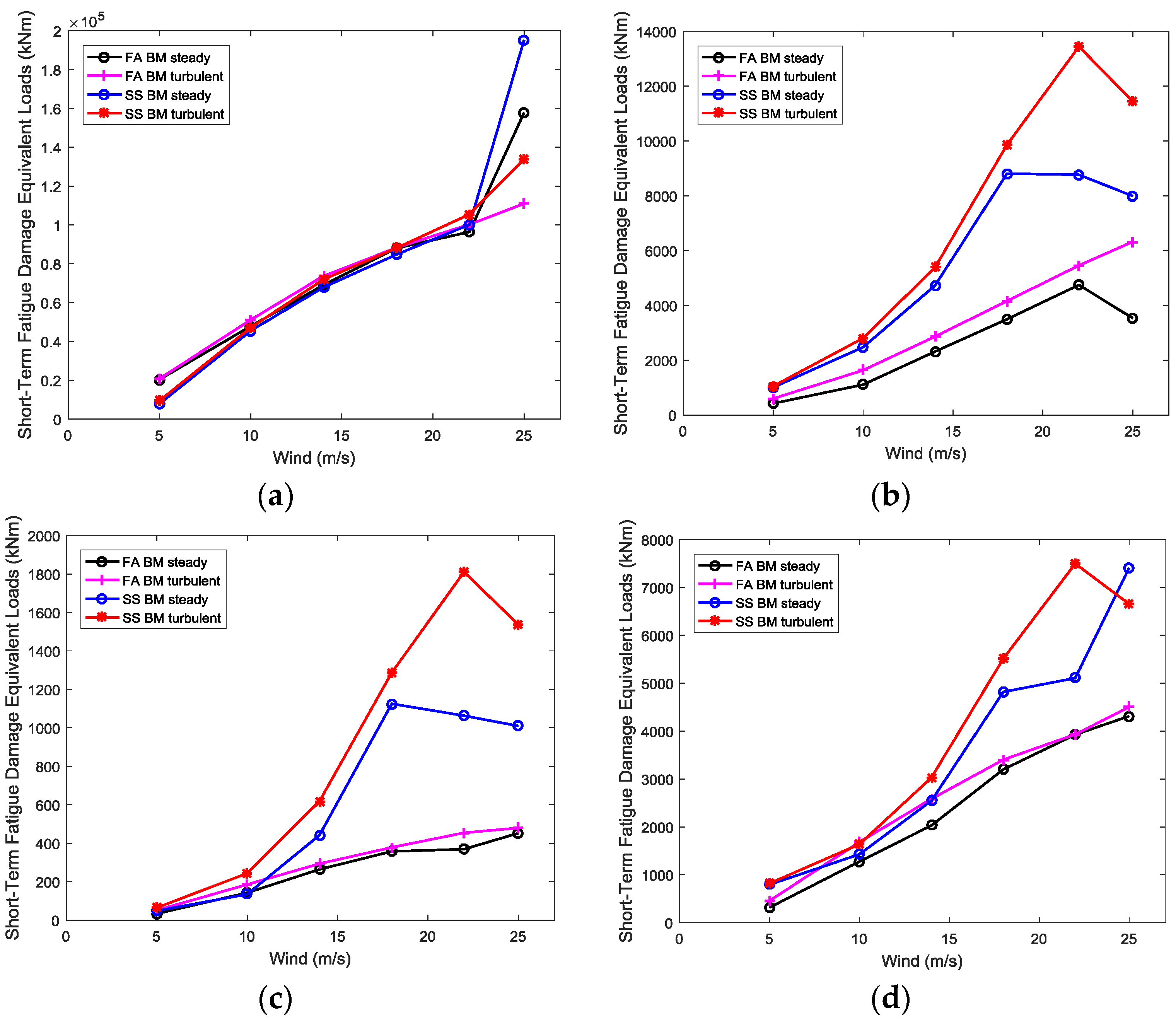
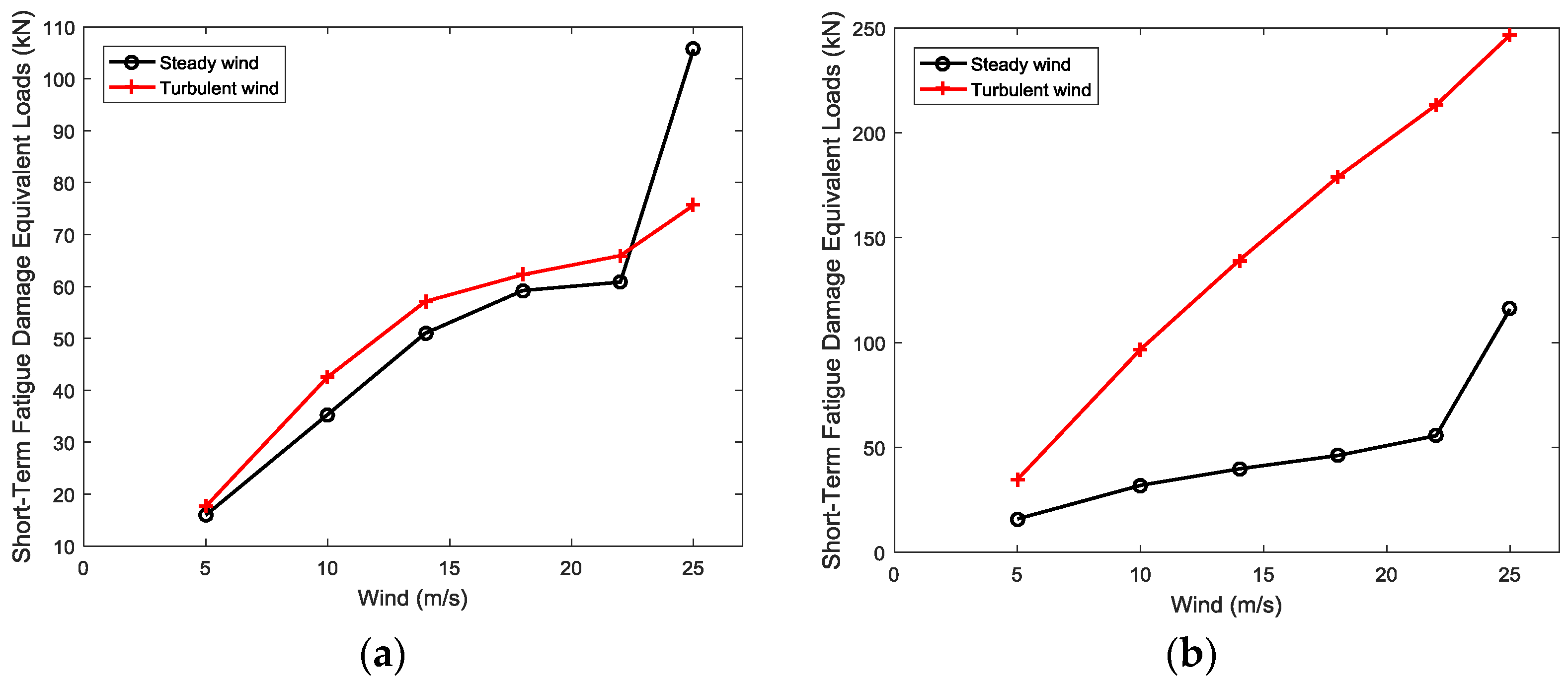
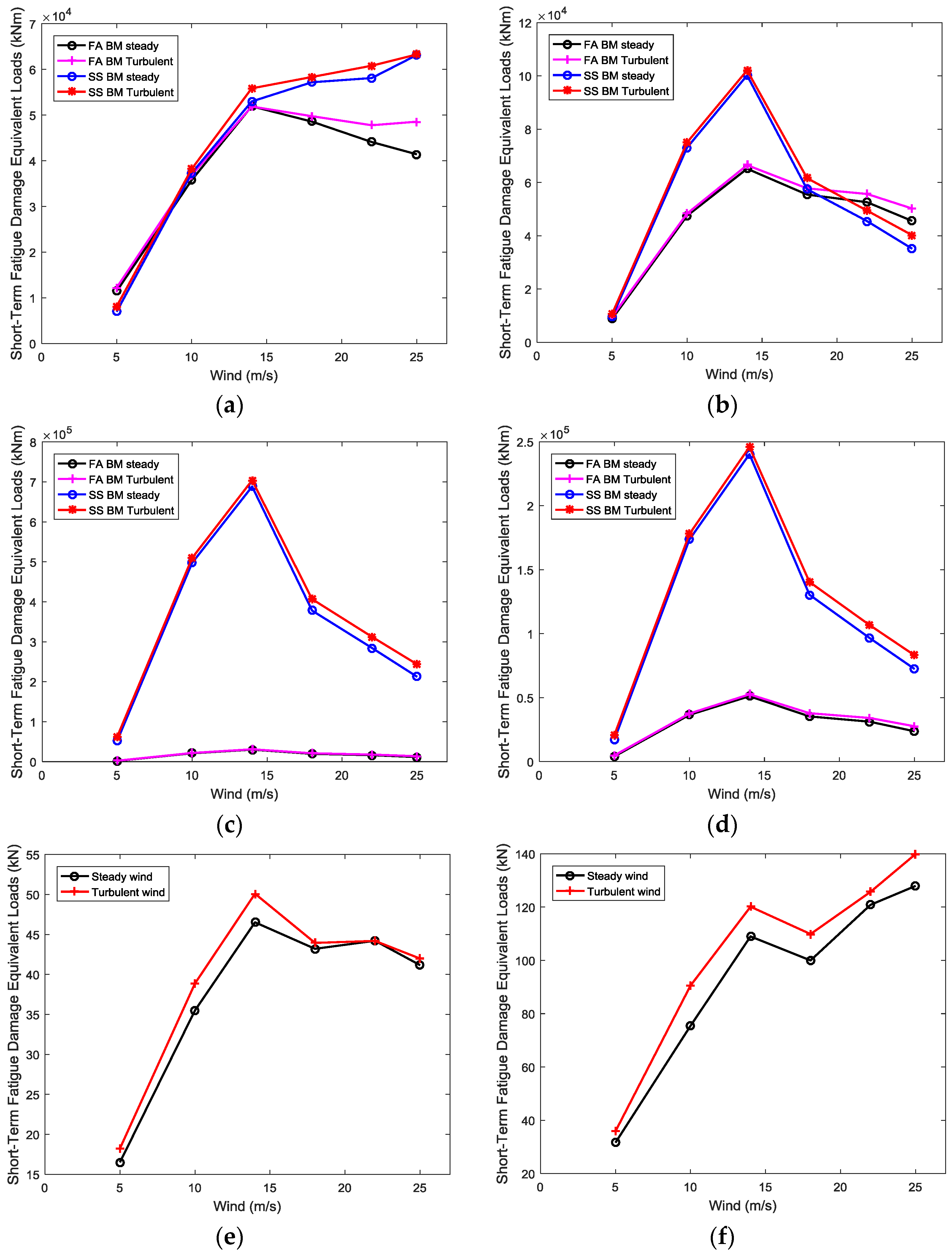
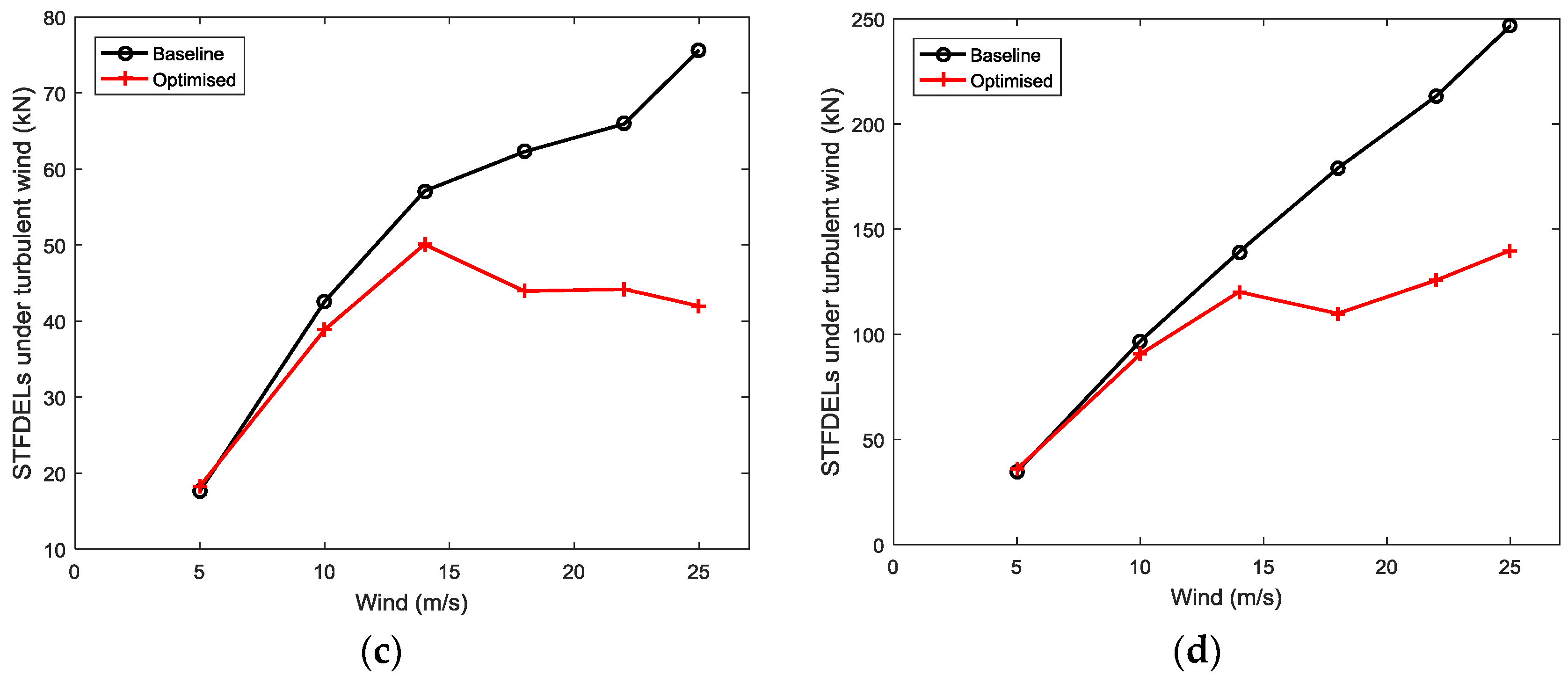
The platform global motions and the structural responses of flexible components of the FVAWTs were studied in a systematic manner under normal operating condition. Furthermore, the fatigue analysis of flexible components such as blades, tower and mooring lines were performed based on the time history of calculated responses considering the continuously varying aerodynamic loads on the rotor which leads to higher load level of the fatigue loads and number of load cycles. The rainflow counting technique is used for short-term fatigue cycle counting. The Mlife tool from NREL is used to calculate the short-term fatigue damage equivalent loads for the FVAWT.
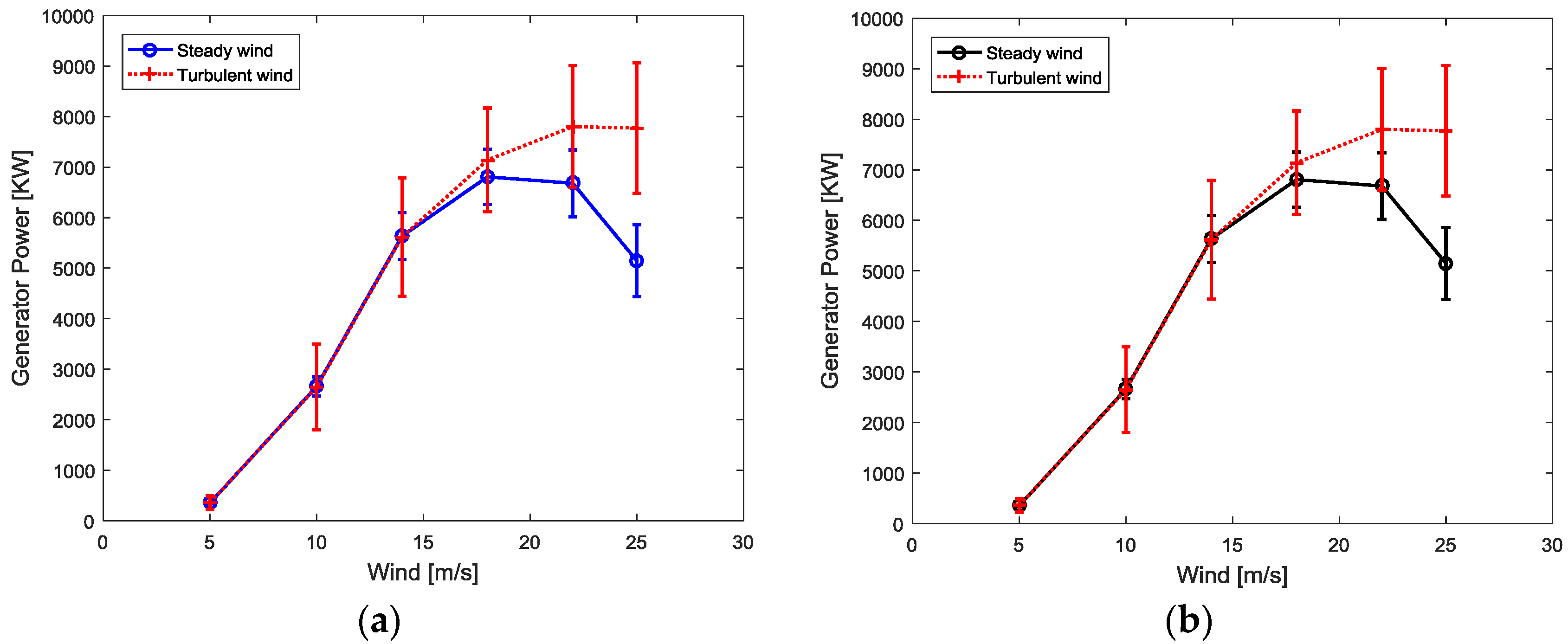
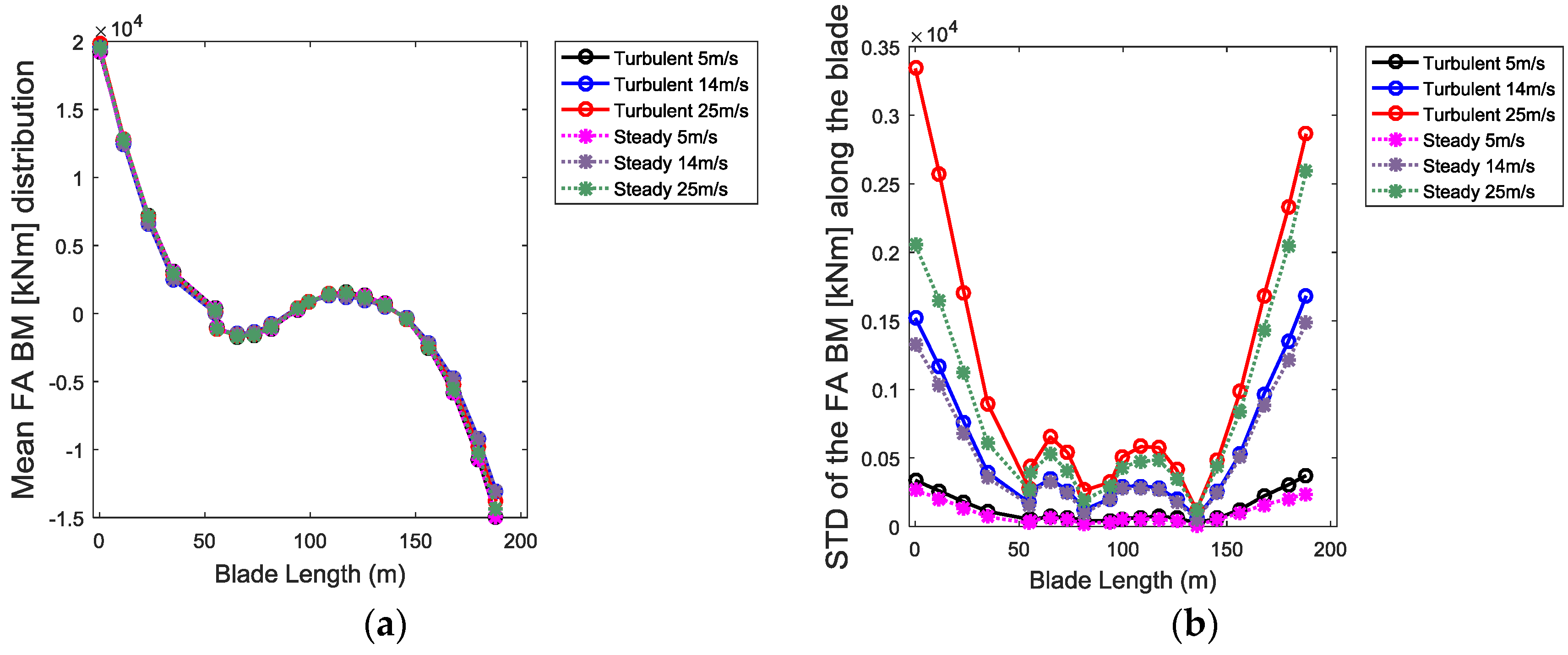
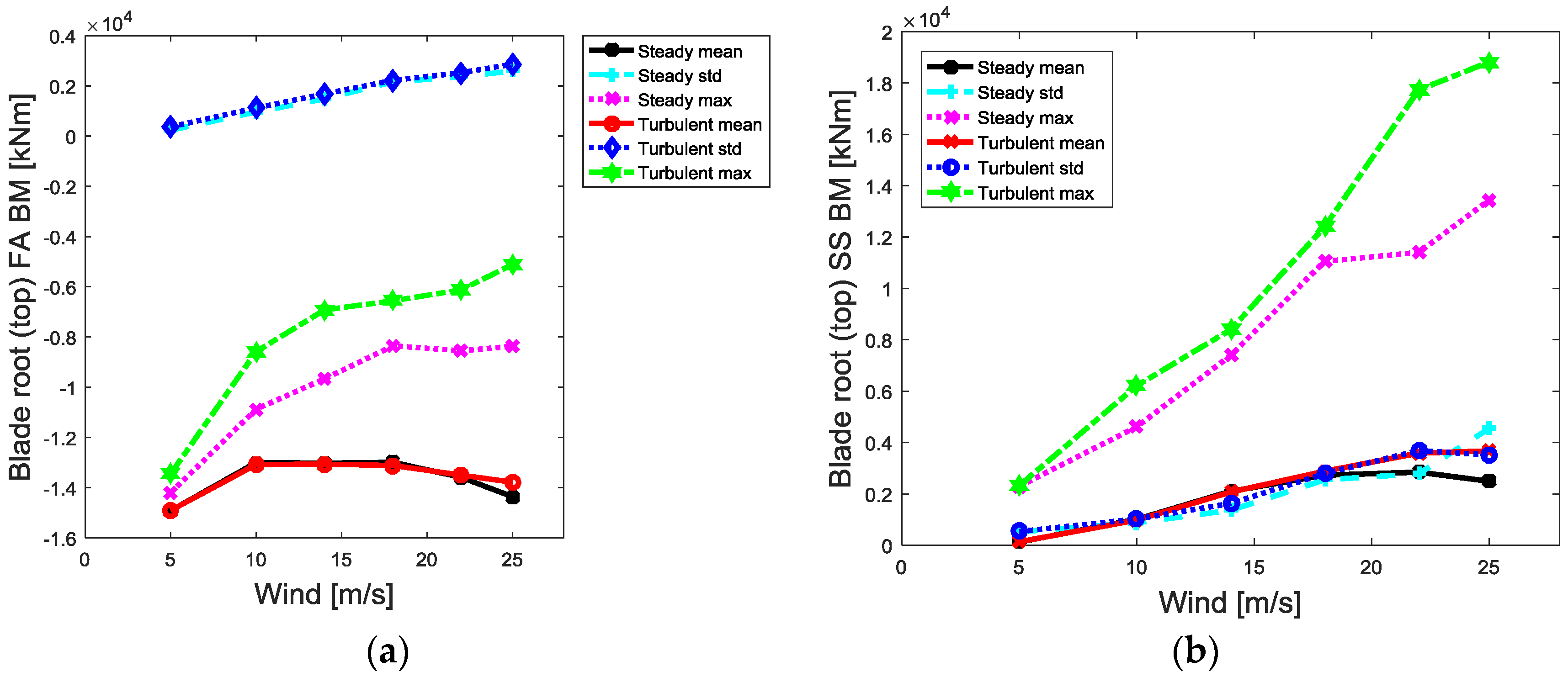
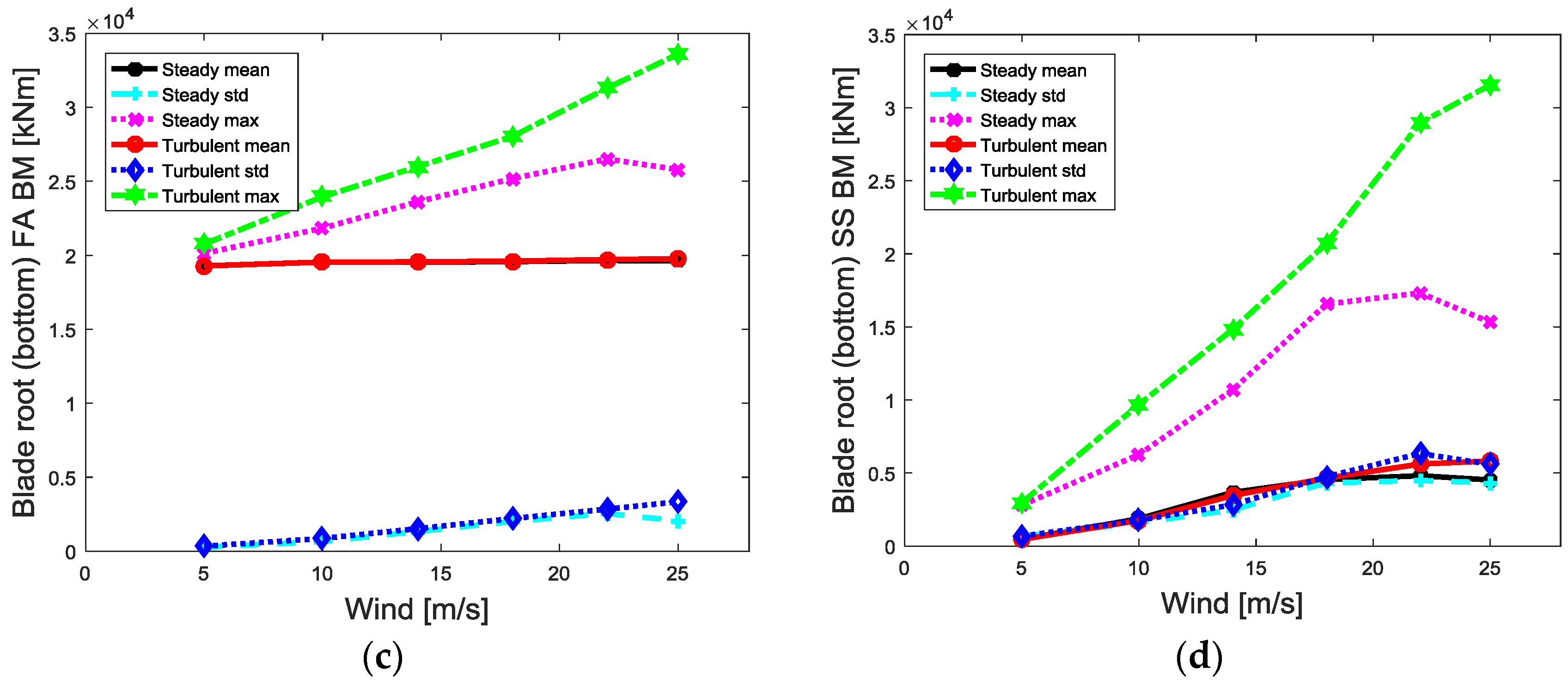
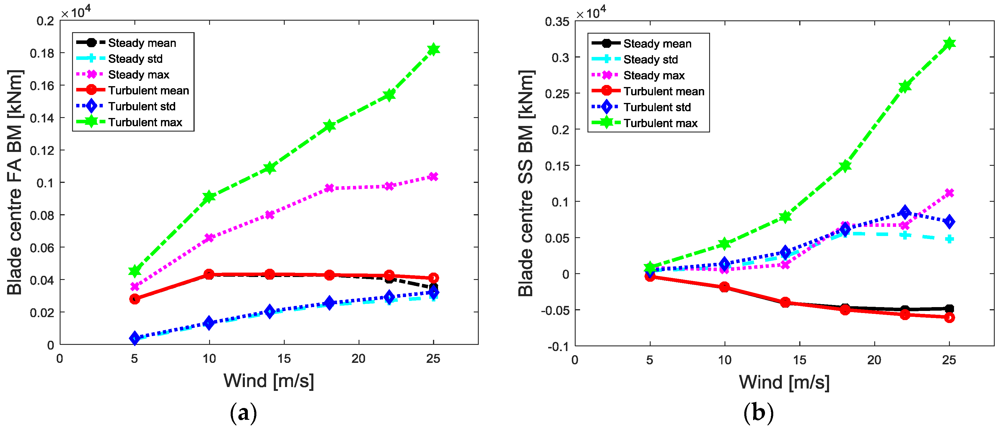
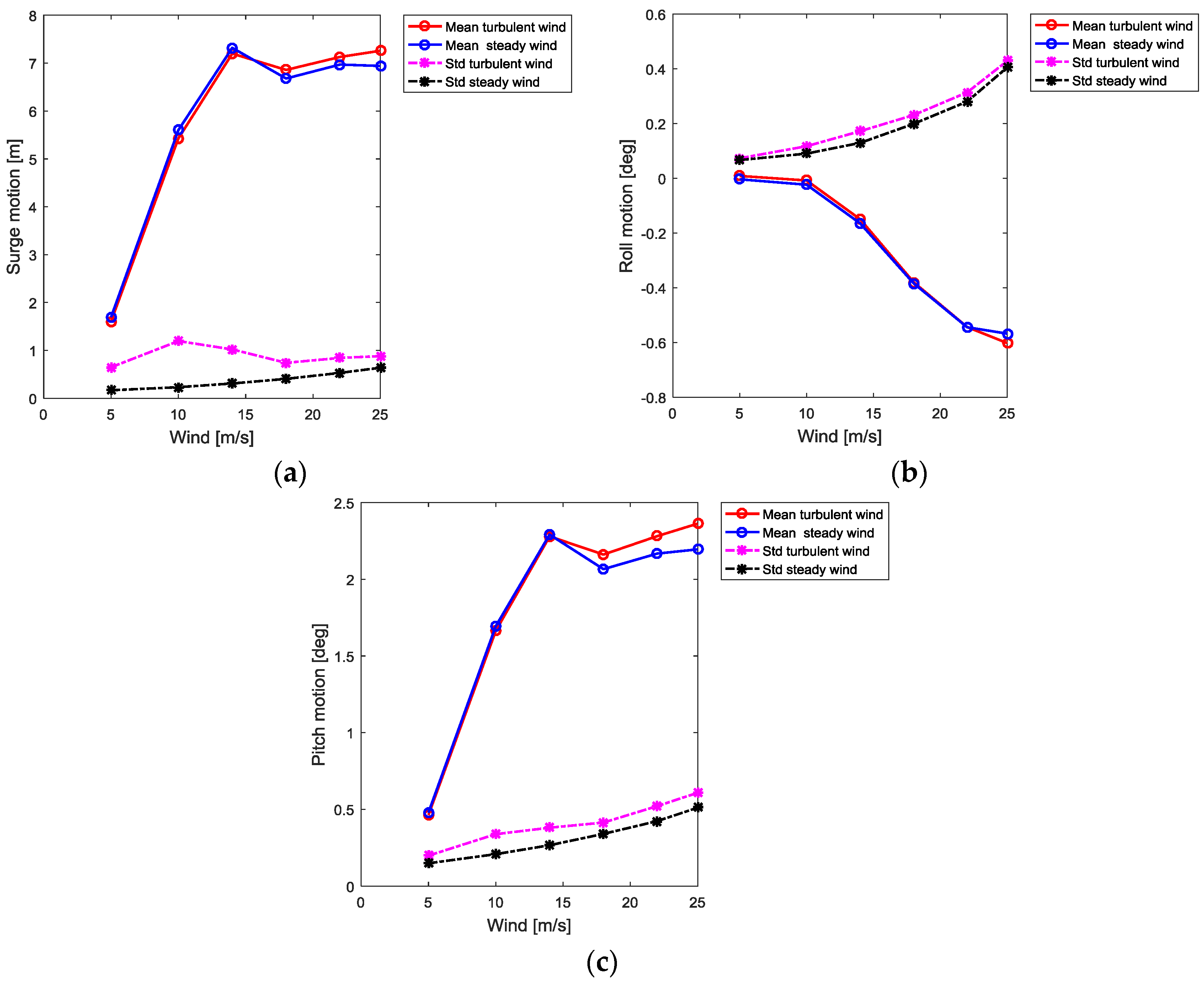
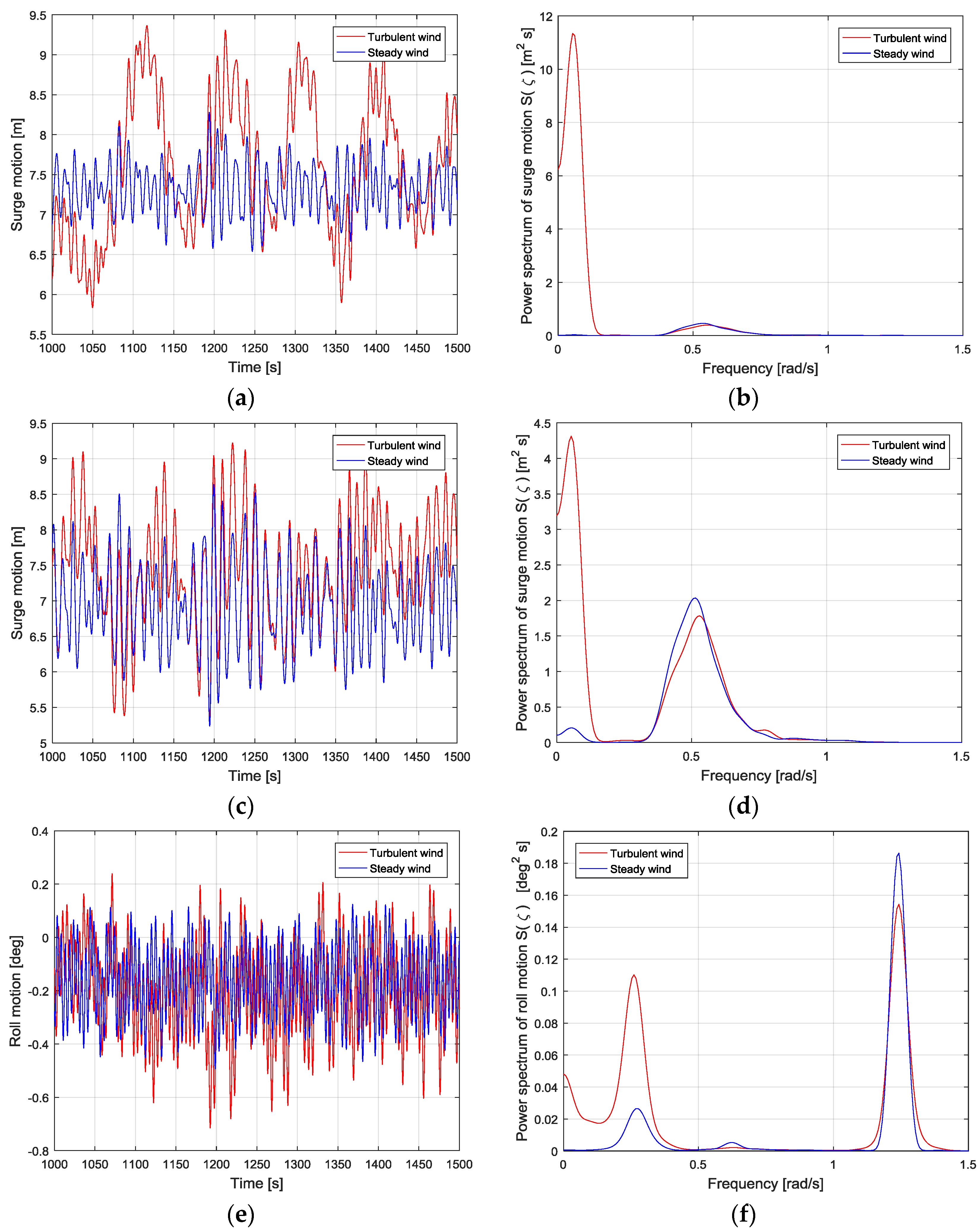
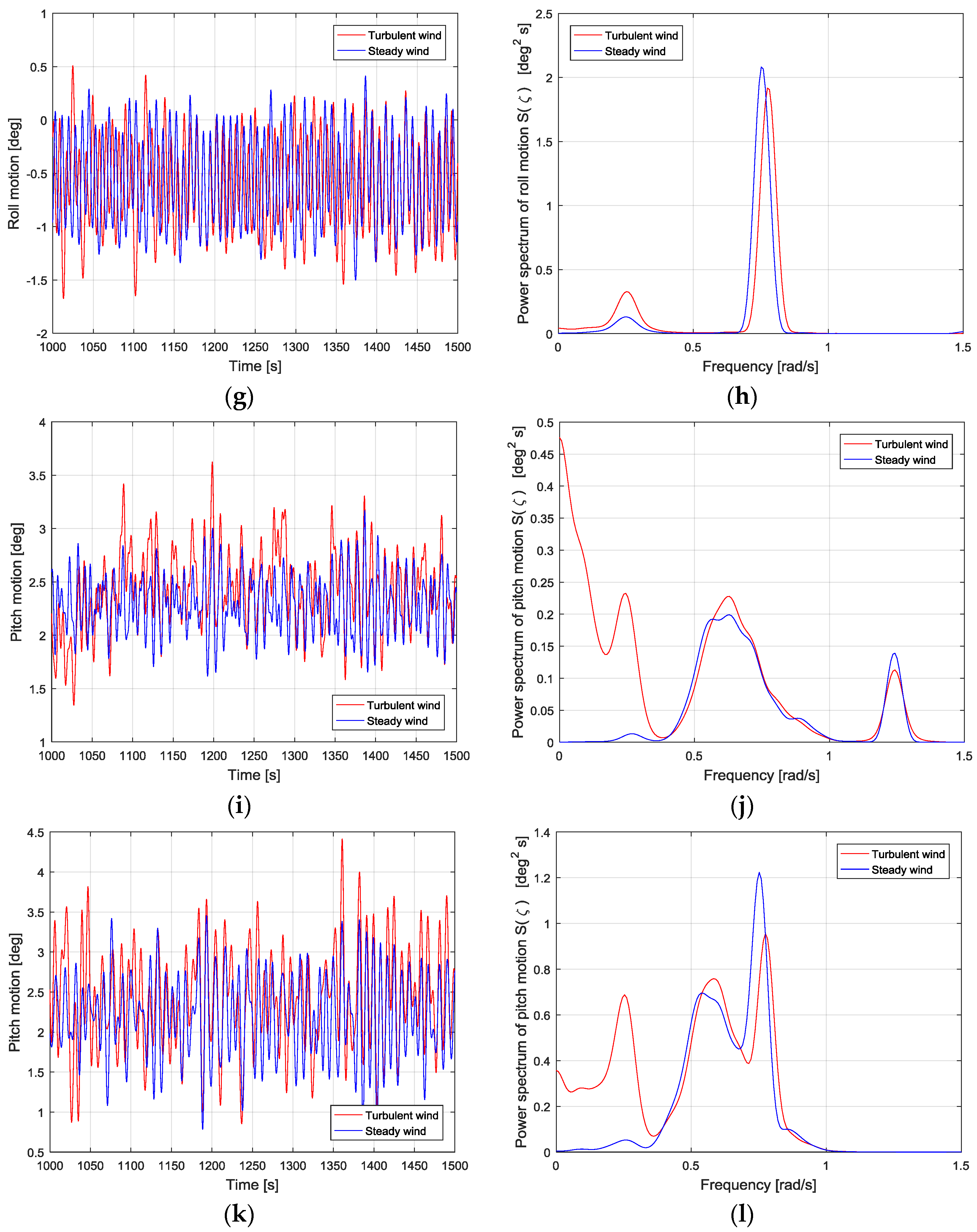
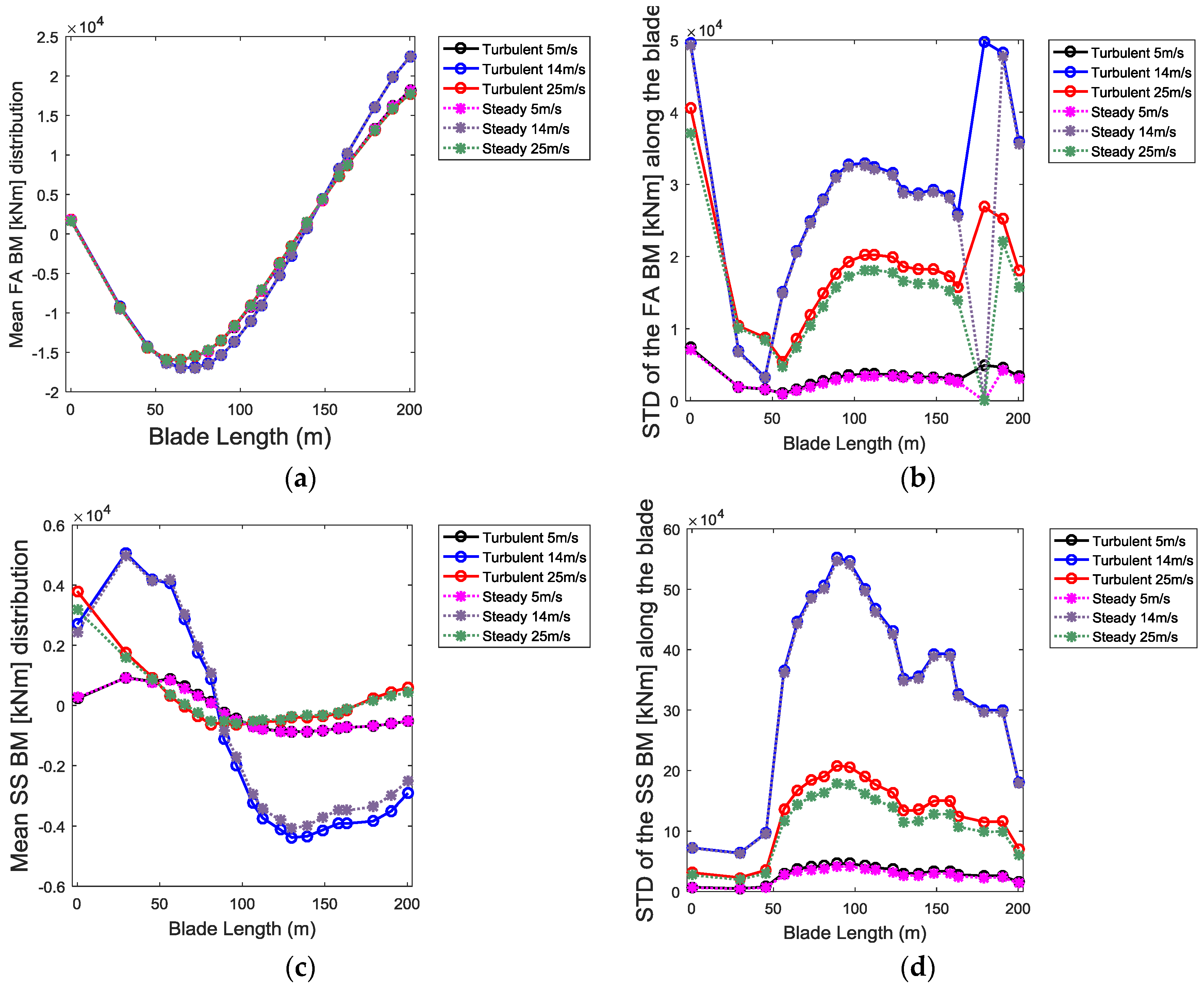
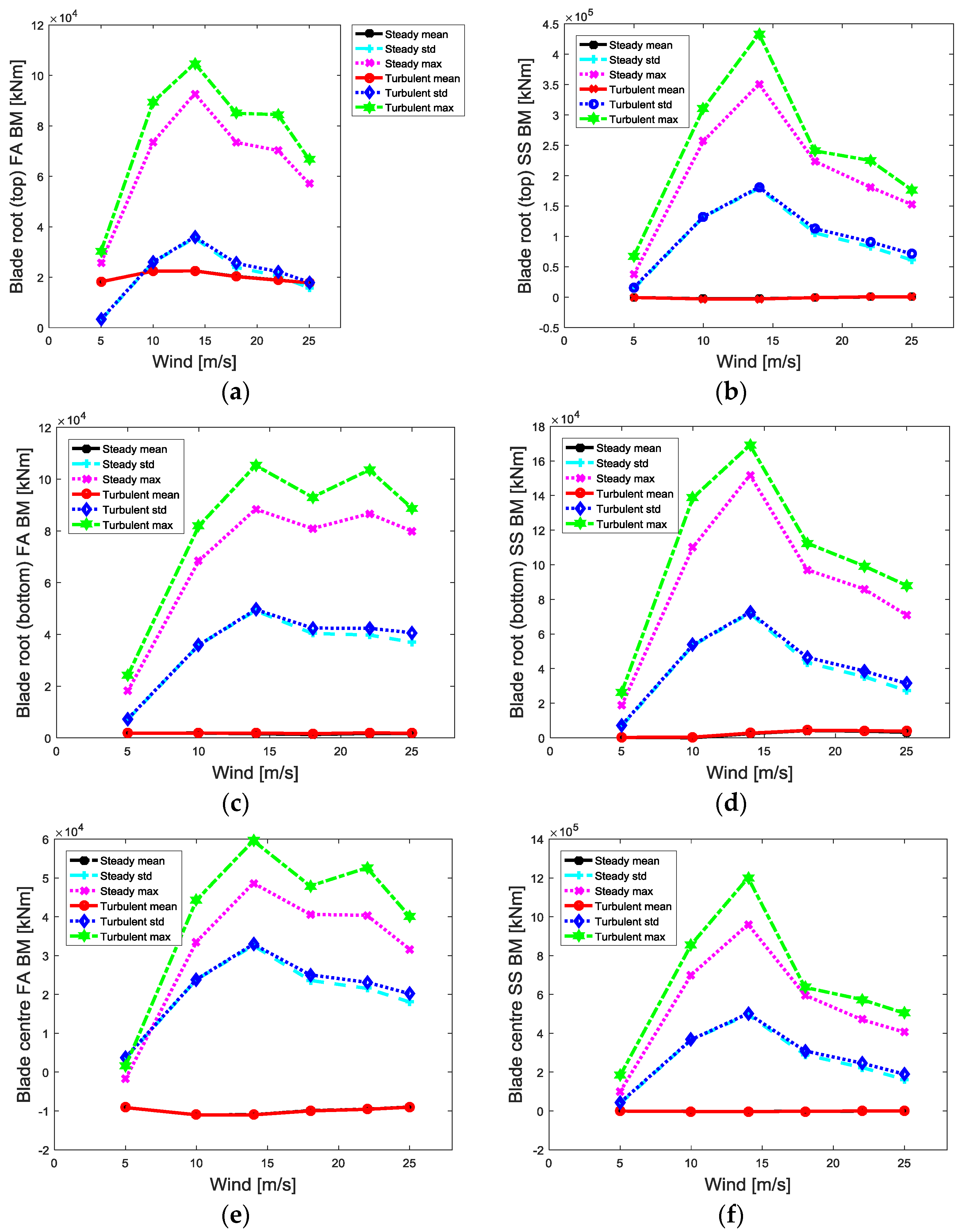
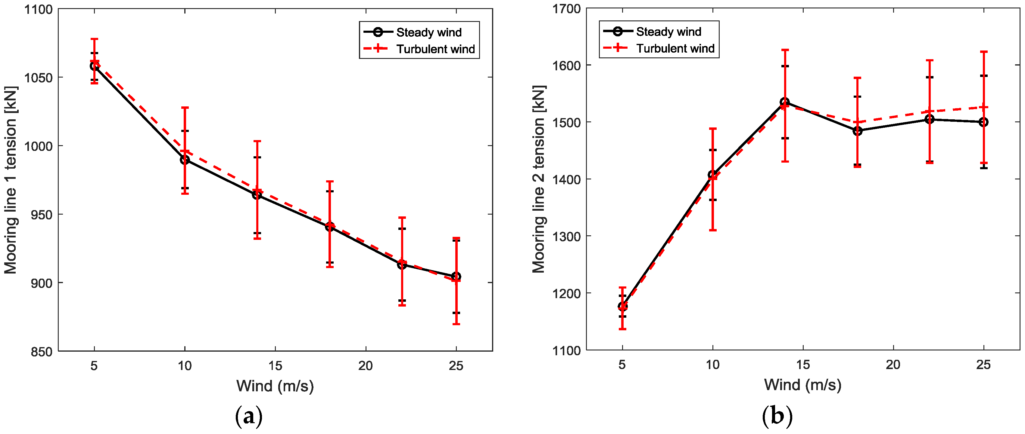
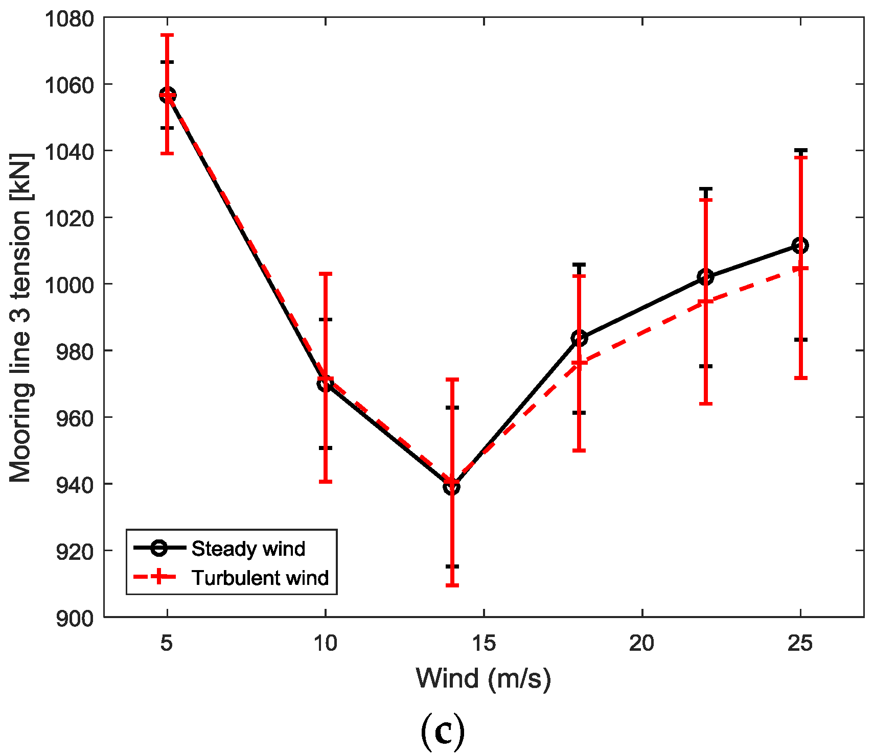
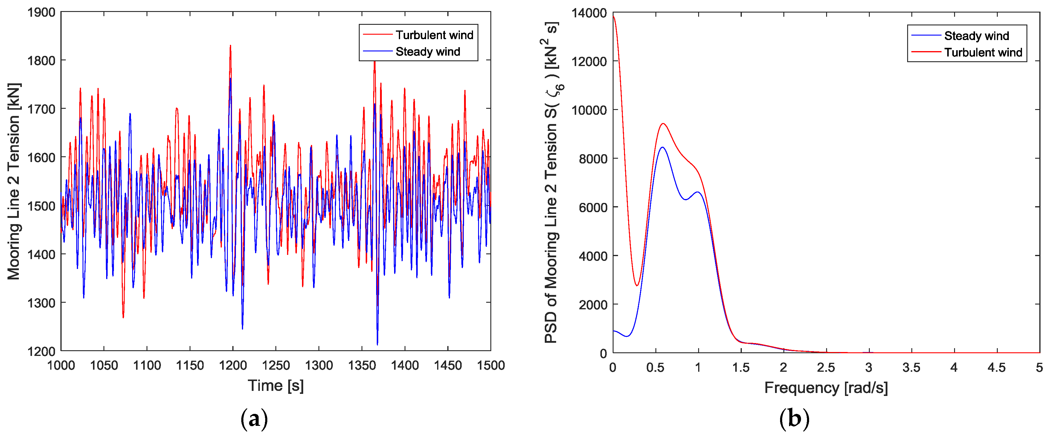
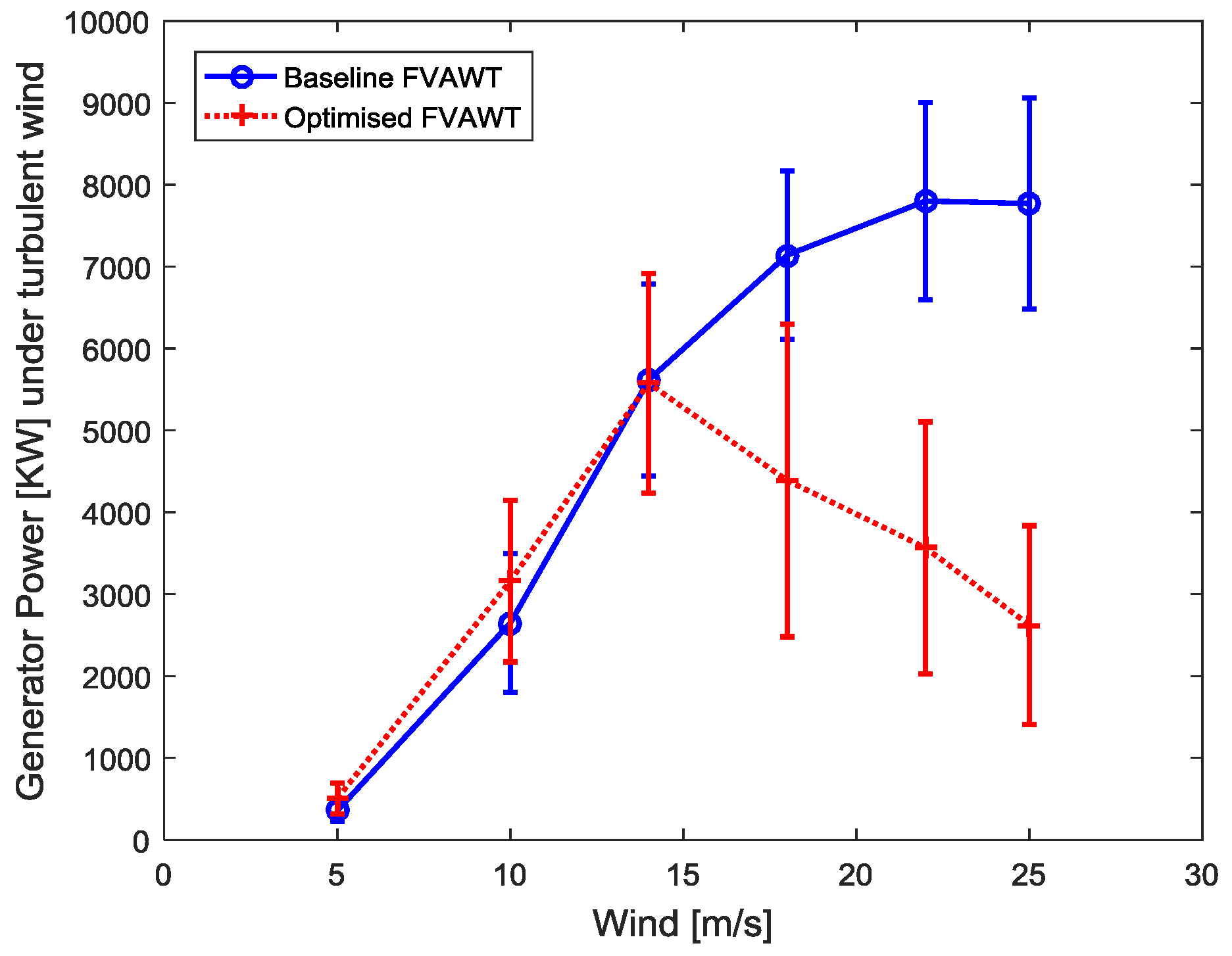
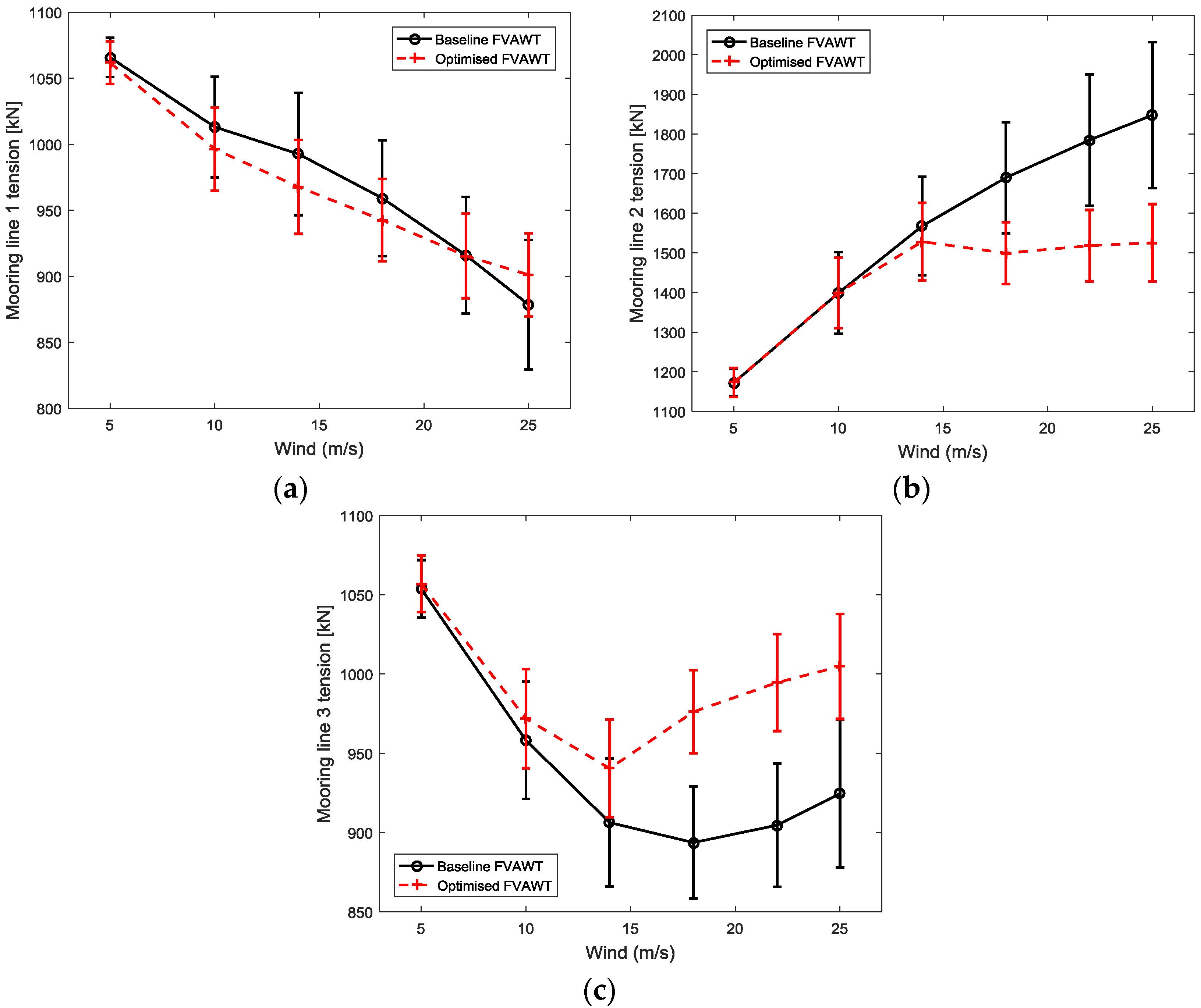
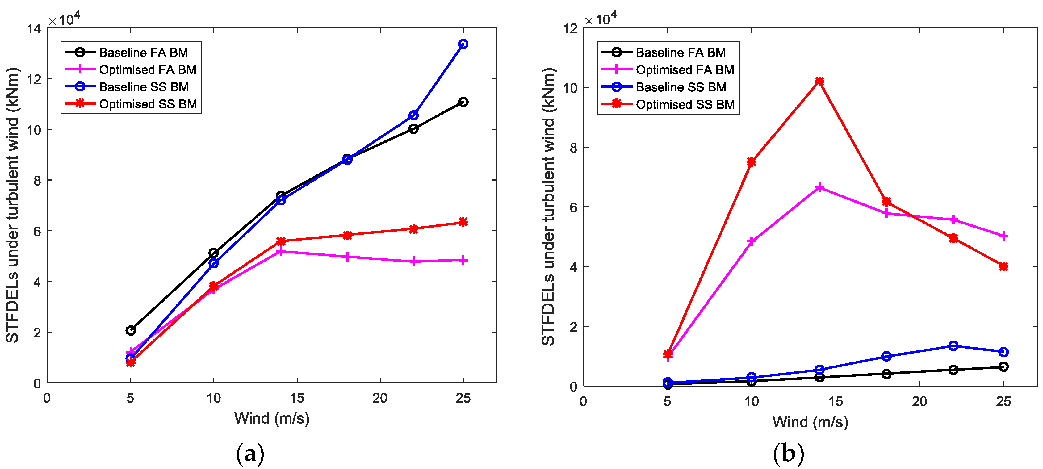
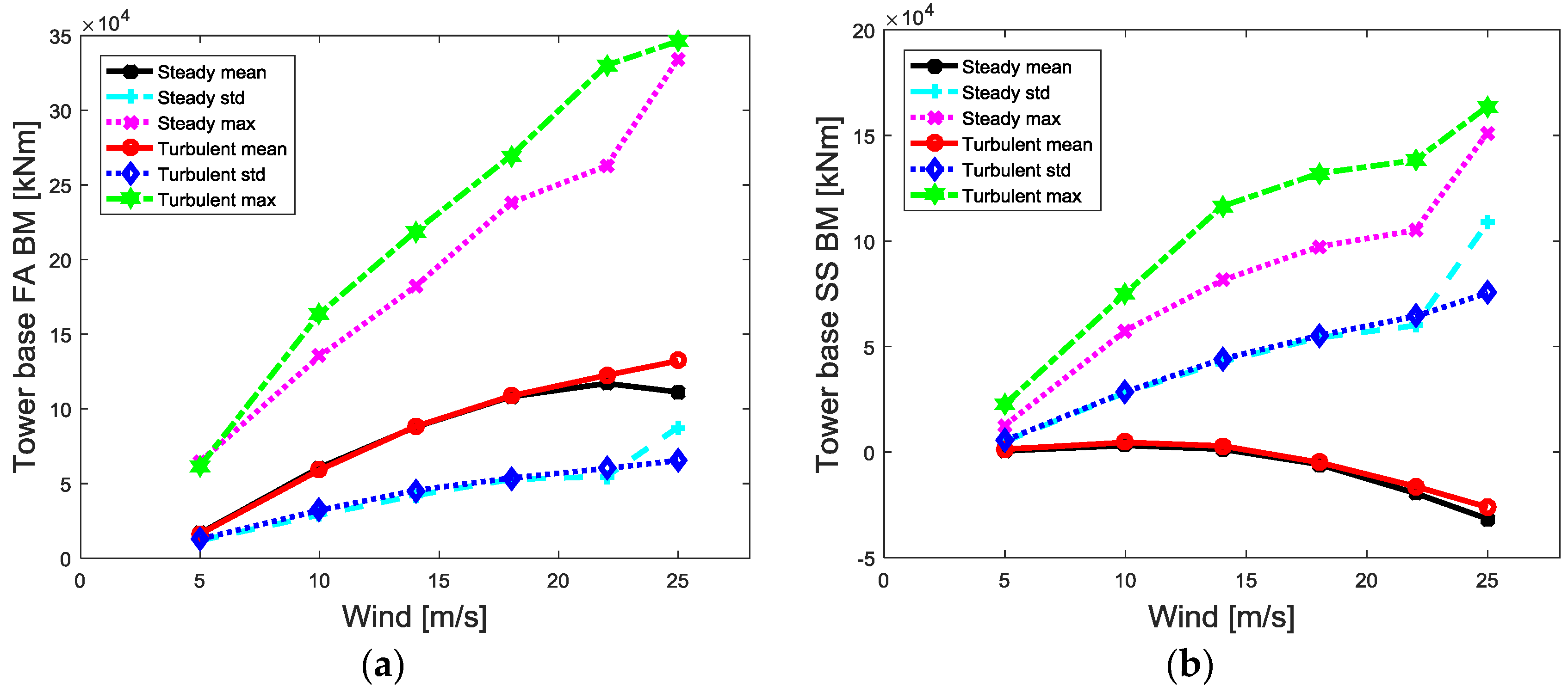
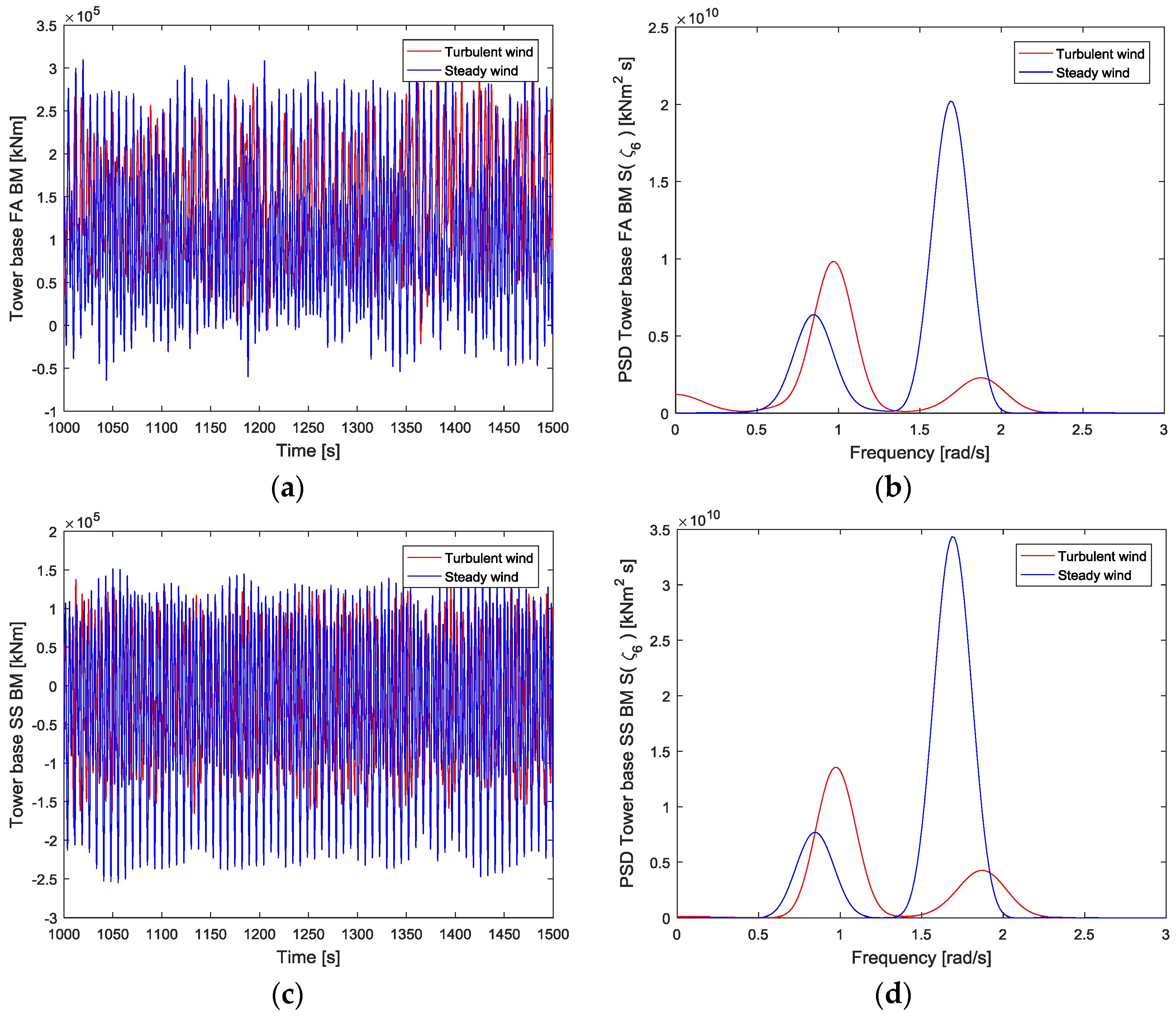
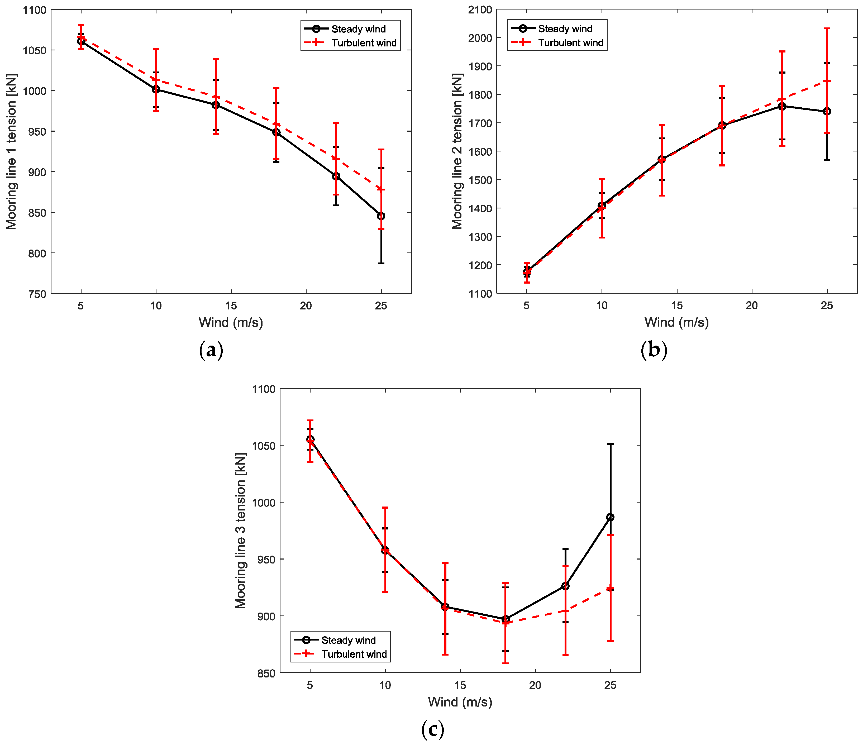
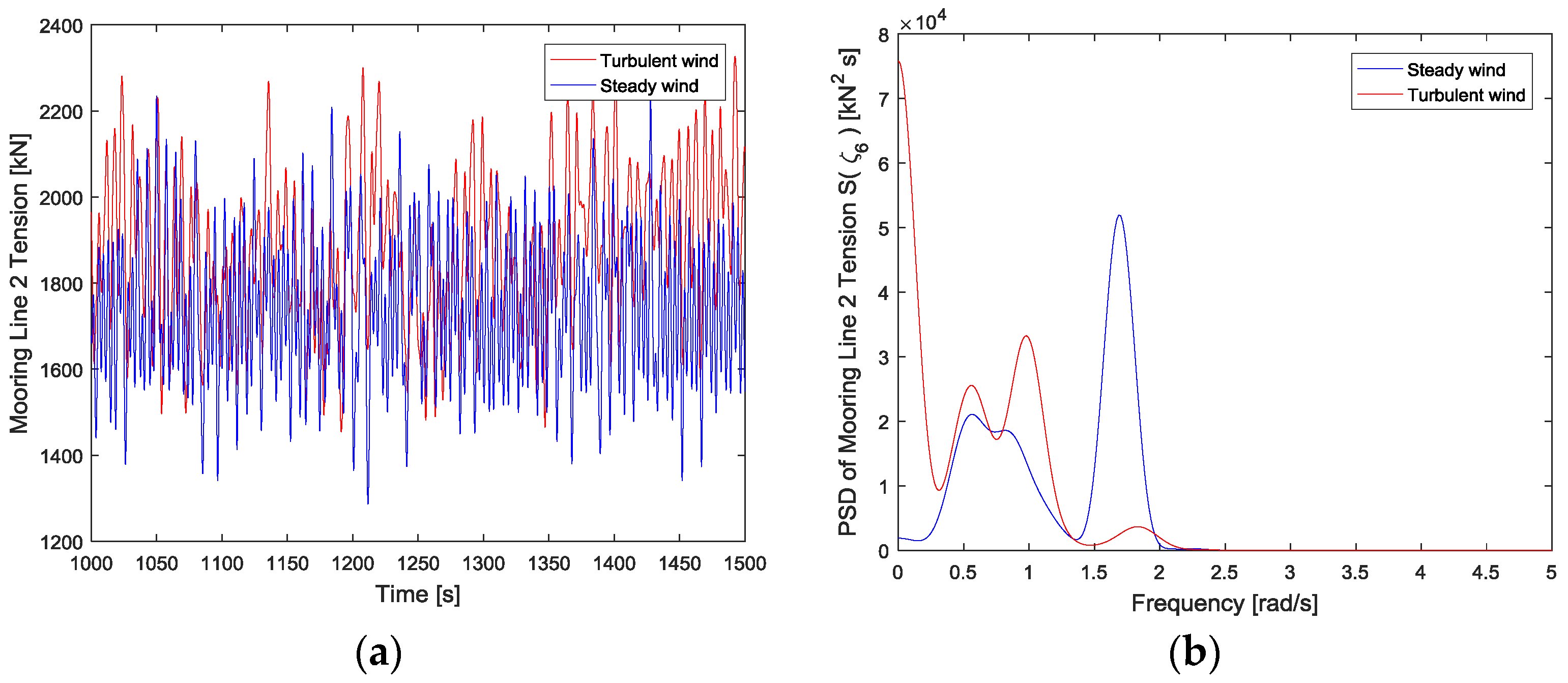
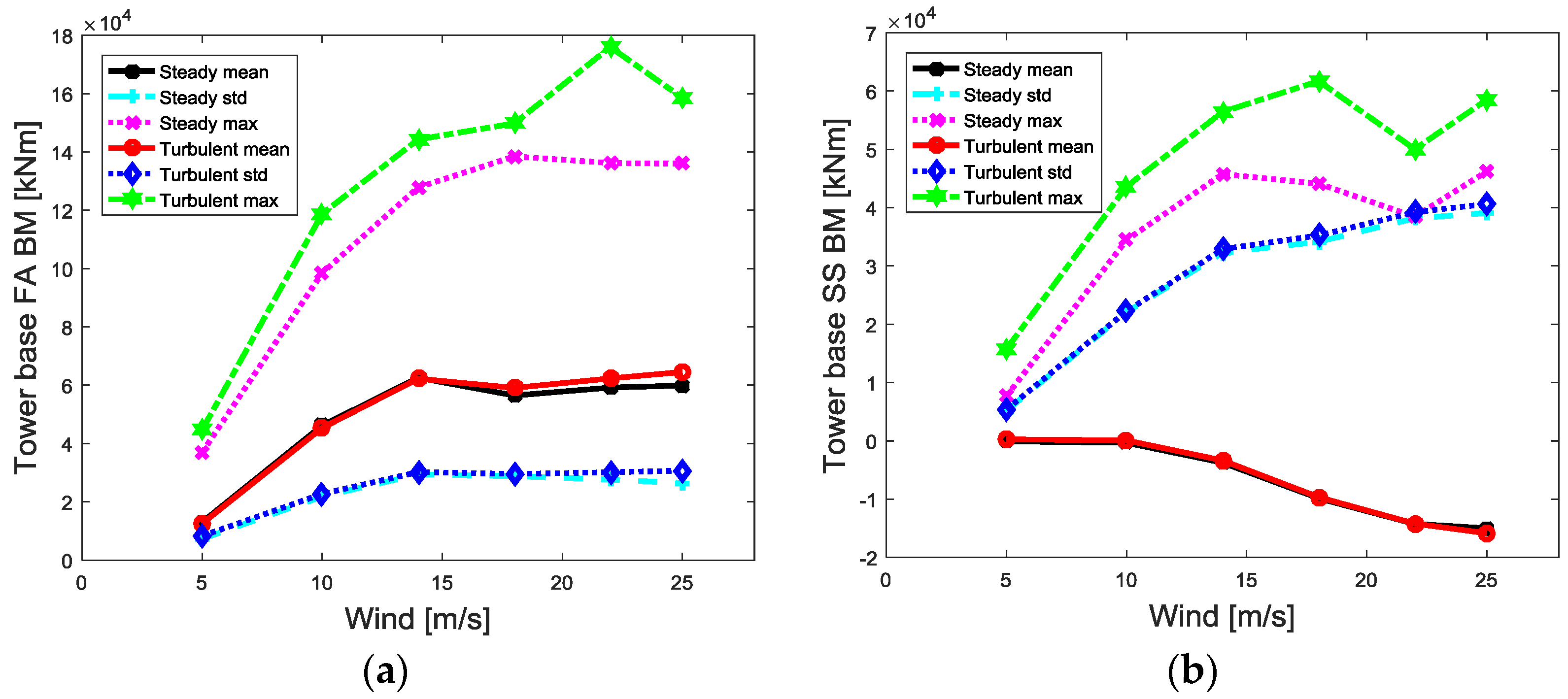
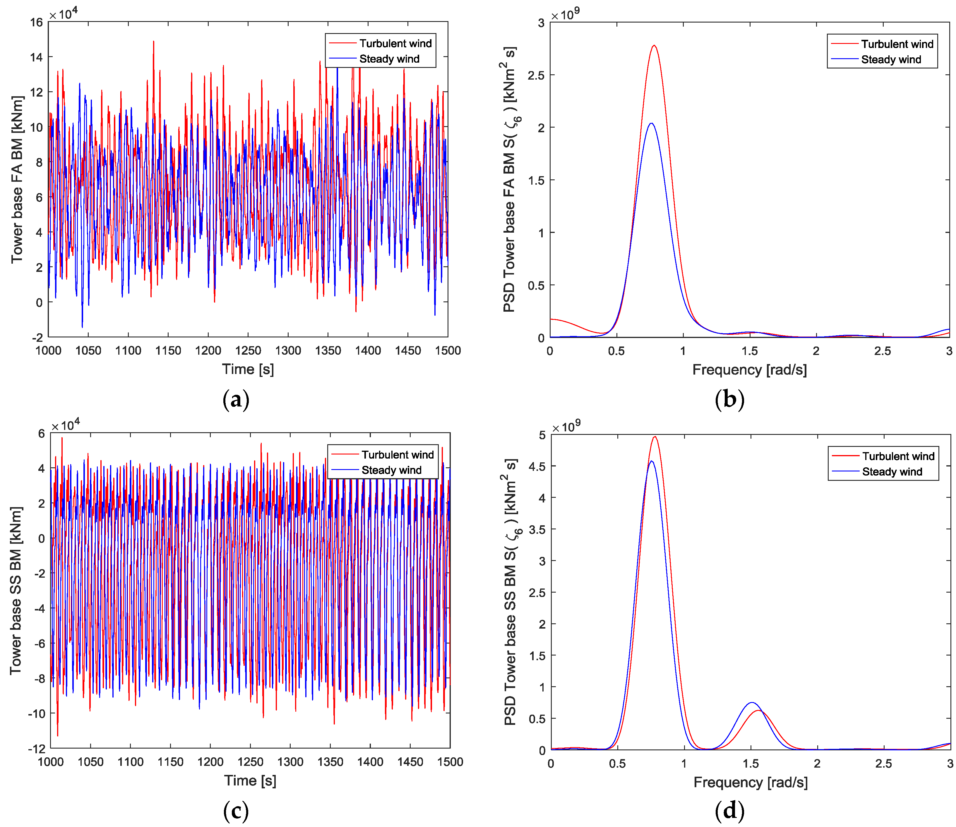
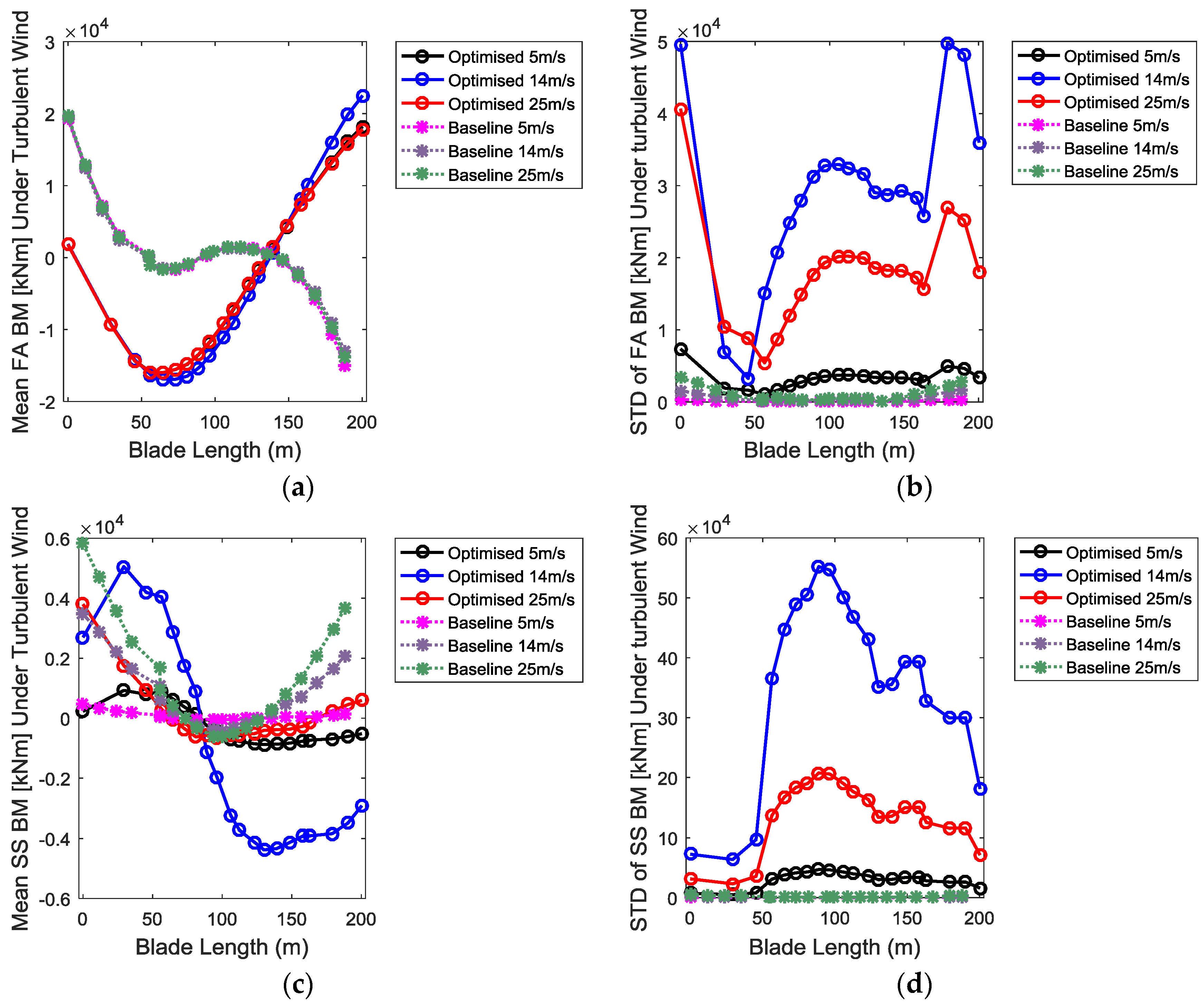
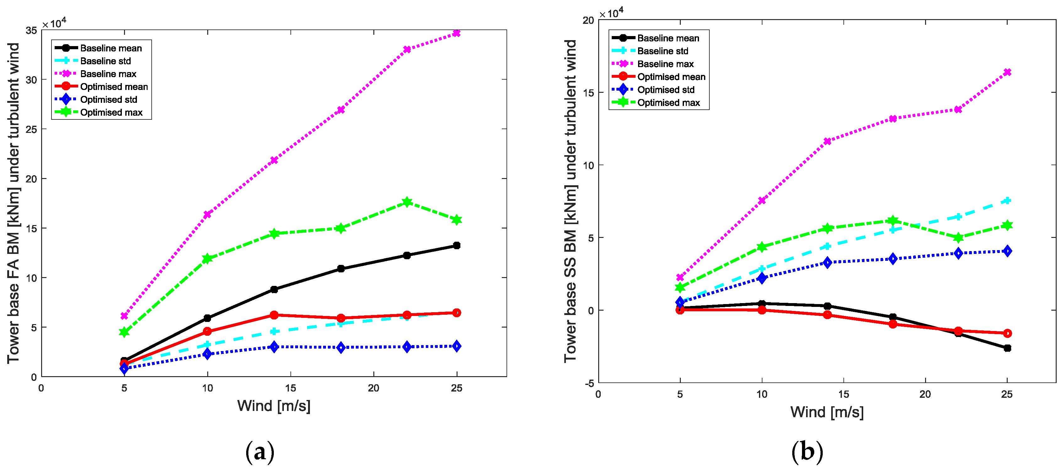
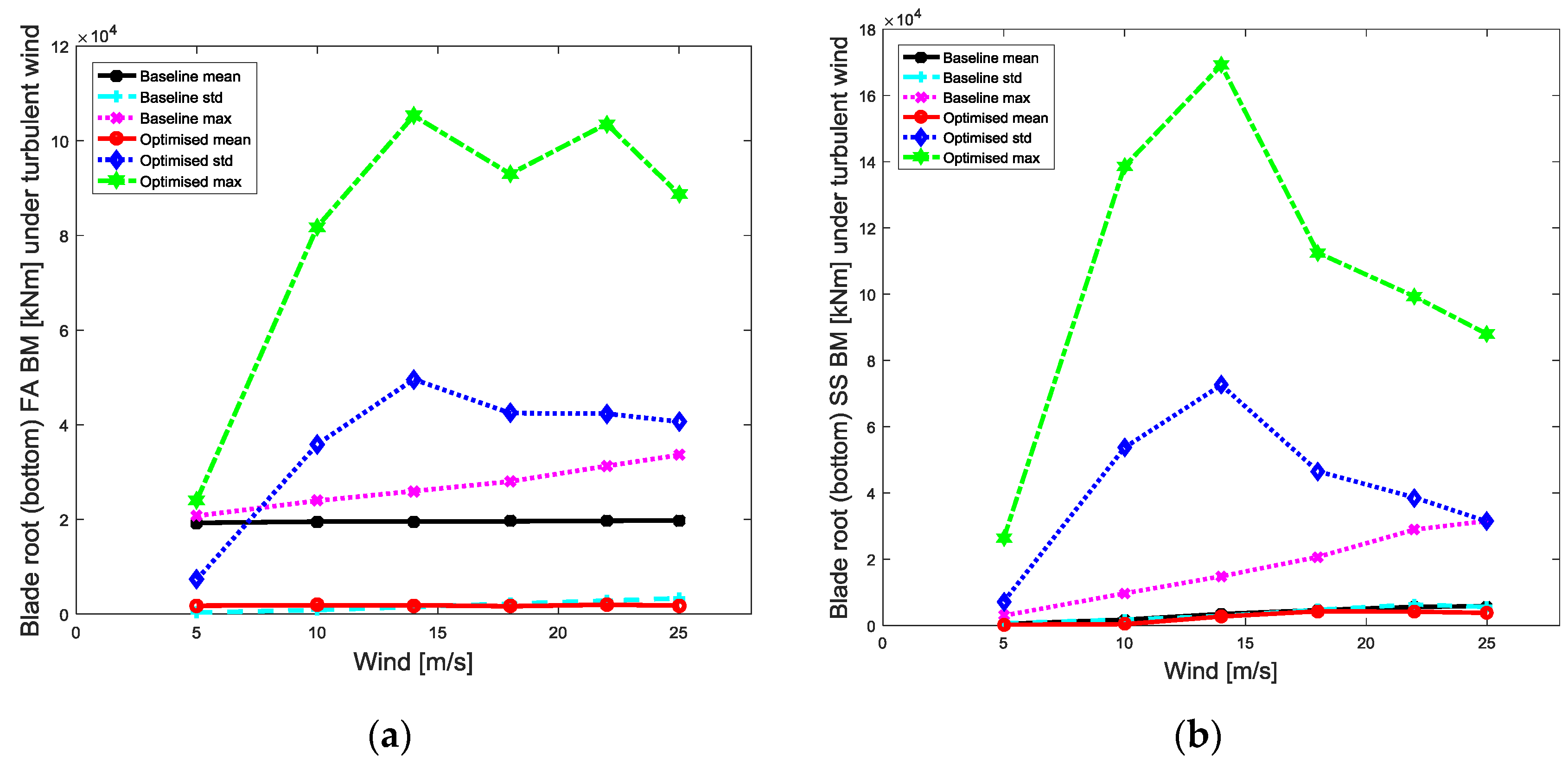
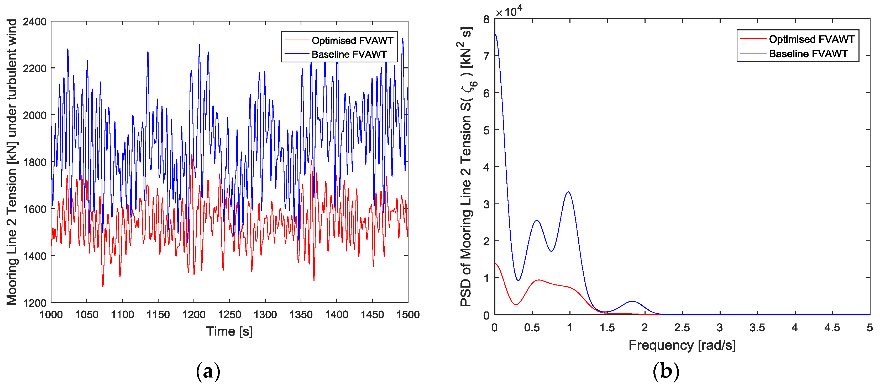
The two FVAWT concepts were evaluated under the same environmental conditions. The stochastic response characteristics of both FVAWTs were studied under steady wind and turbulent wind conditions based on the statistical analysis and the spectral analysis of their responses to explore the effects of turbulence. The results identified that the effect of turbulence on the both FVAWTs resulted in an increased power generation, higher power variation, higher excitation for low frequency motions, greater fatigue damage but a reduction in the 2P effects. However, the effect of turbulence is negligible on the mean bending moment at the blade extremes but leads to higher loads level in mooring lines and at the tower base especially at wind speeds above the rated wind speed. Furthermore, the results of the fatigue analysis showed that at wind speeds farther from the rated wind speed (14 m/s), the internal loads could have lower damaging effects than at wind speeds closer to the rated wind speed for the 5 MW optimised FVAWT.
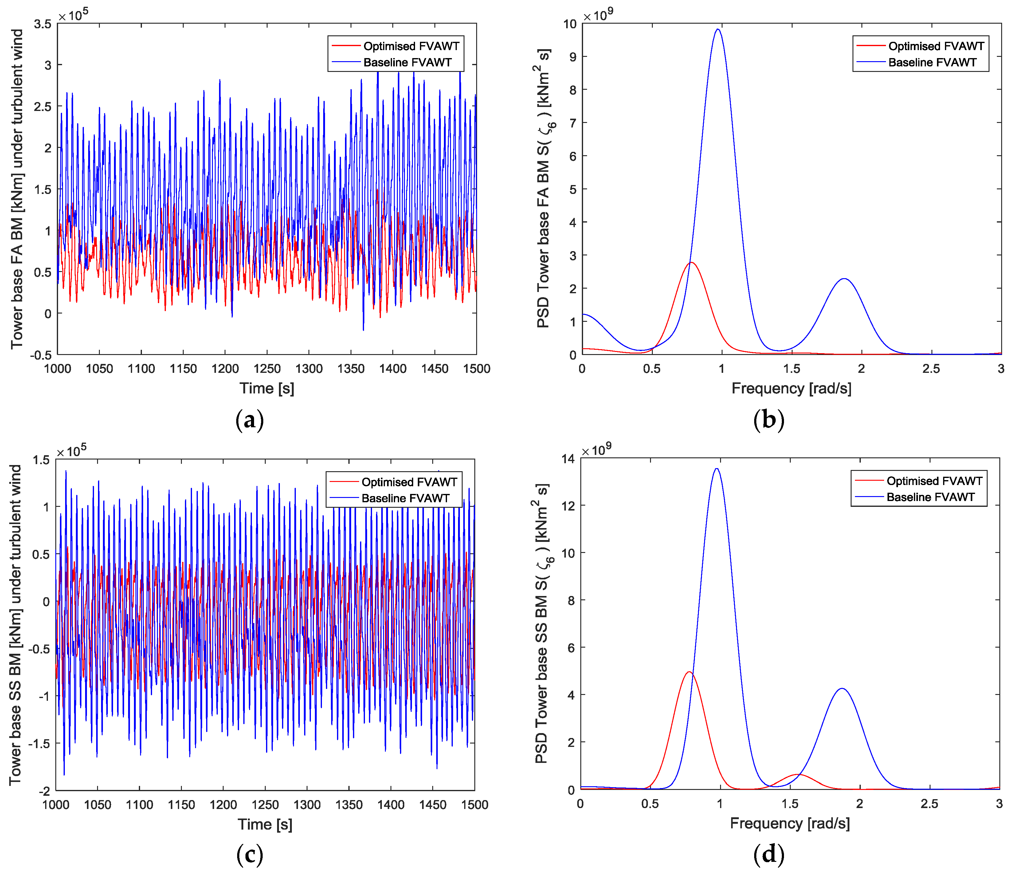
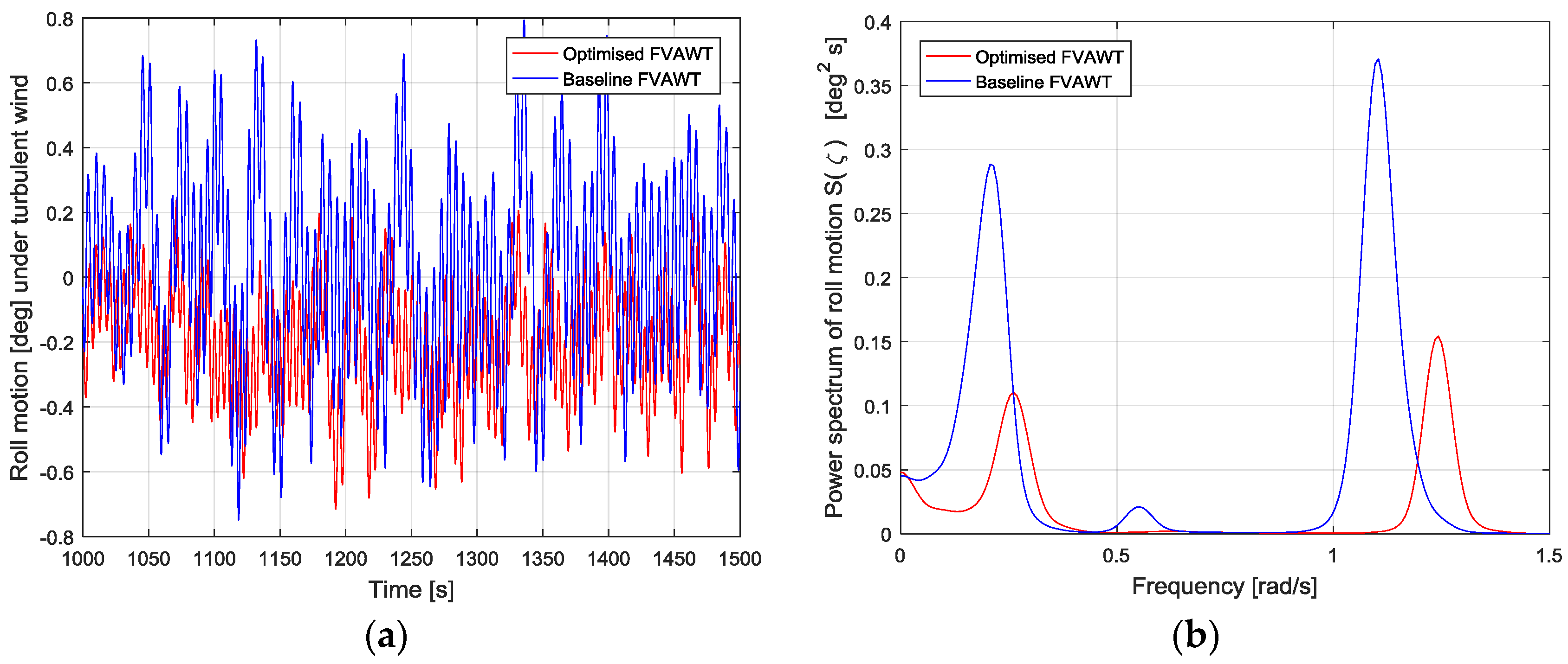
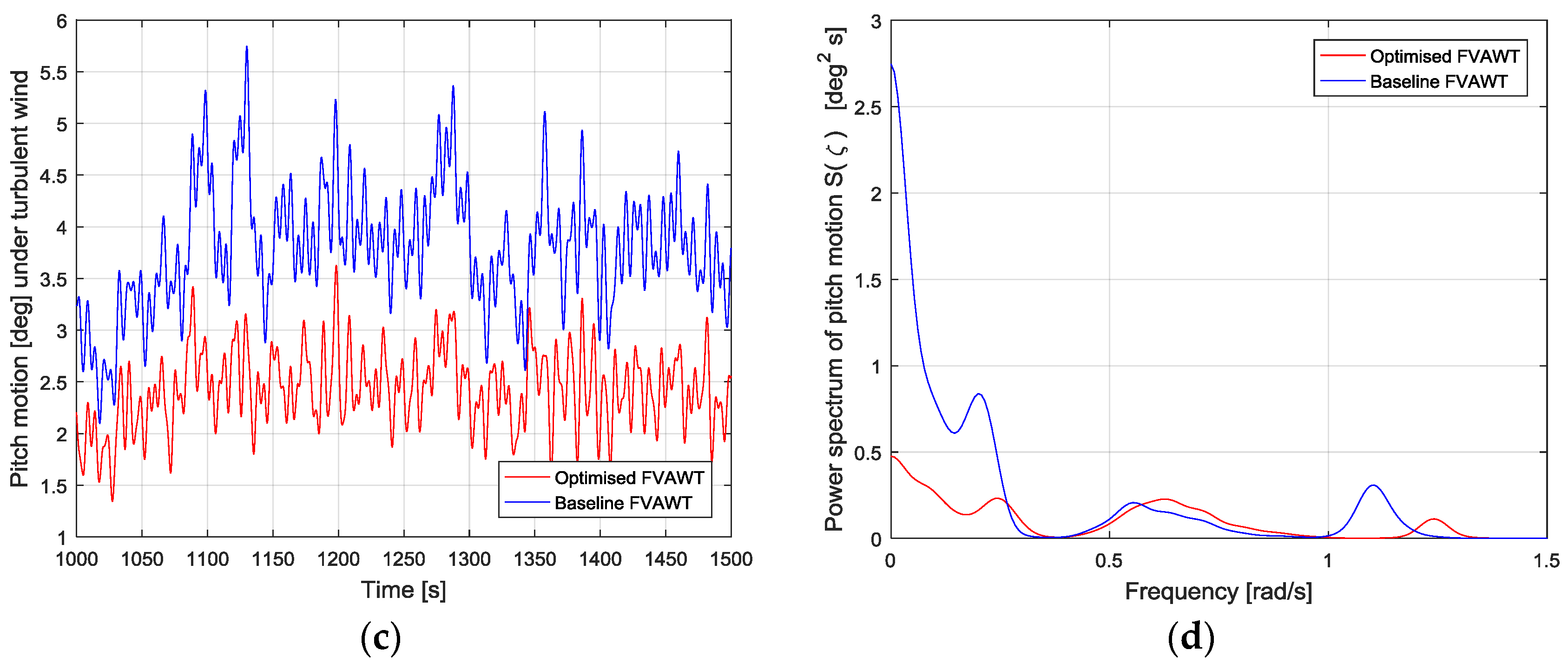
Finally, a comparison of dynamic responses between the 5 MW baseline FVAWT and the 5 MW optimised FVAWT identified the 5 MW optimised FVAWT to have lower Fore-Aft (FA) bending moments but higher lower Side-Side (SS) bending moment in flexible components, lower motions amplitude, lower short-term fatigue damage equivalent loads and a further reduced 2P effects under turbulent wind condition.

Author Contributions

Kai Wang and Muk Chen Ong conceived and designed the numerical study; Kai Wang and Jeremiah Ishie contributed analysis tools; Jeremiah Ishie performed the numerical simulations under the supervision of Kai Wang and Muk Chen Ong; Jeremiah Ishie analyzed the data with the comments from Kai Wang and Muk Chen Ong; Jeremiah Ishie wrote the paper under the supervision of Kai Wang and Muk Chen Ong; Kai Wang and Muk Chen Ong gave comments and modified the paper.

Conflicts of Interest

The authors declare no conflict of interest.

Abbreviations

FA BMFore-Aft bending moment (bending parallel to the wind direction)
SS BMSide-side bending moment (along a direction at 90° to the wind direction)
STFDELShort-Term Fatigue Damage Equivalent Load
FA BM steadySTFDEL due to FA BM under steady wind condition
FA BM turbulentSTFDEL due to FA BM under turbulence wind condition
SS BM steadySTFDEL due to SS BM under steady wind condition
SS BM turbulentSTFDEL due to SS BM under turbulence wind condition
steadySTFDEL due to axial force or tension under steady wind condition
turbulentSTFDEL due to axial force or tension under turbulent wind condition
Optimized FA BM STFDEL due to FA BM for the 5 MW optimized FVAWT
Baseline FA BMSTFDEL due to FA BM for the 5 MW baseline FVAWT
Optimized SS BMSTFDEL due to SS BM for the 5 MW optimized FVAWT
Baseline SS BMSTFDEL due to SS BM for the 5 MW baseline FVAWT
Optimized STFDEL due to axial force for the 5 MW optimized FVAWT
Baseline STFDEL due to axial force for the 5 MW baseline FVAWT

References

  1. Paquette, J.; Barone, M.; Paquette, J.; Barone, M. Innovative offshore vertical-axis wind turbine rotor project. In Proceedings of the EWEA 2012 Annual Event, Copenhagen, Denmark, 16–19 April 2012.
  2. Wang, K.; Luan, C.; Moan, T.; Hansen, M.O.L. Comparative Study of a FVAWT and a FHAWT with a Semi-submersible Floater. In Proceedings of the Twenty-fourth International Offshore and Polar Engineering Conference, Busan, Korea, 15–20 June 2014.
  3. Anagnostopoulou, C.; Kagemoto, H.; Sao, K.; Mizuno, A. Concept design and dynamic analyses of a floating vertical-axis wind turbine: Case study of power supply to offshore Greek islands. Ocean Eng. Mar. Energy 2015, 2, 85–104. [Google Scholar] [CrossRef]
  4. Wang, K.; Moan, T.; Hansen, M.O.L. Stochastic dynamic response analysis of a floating vertical-axis wind turbine with a semi-submersible floater. Wind Energy 2016, 19, 1853–1870. [Google Scholar] [CrossRef]
  5. Jiang, Z.; Karimirad, M.; Moan, T. Dynamic response analysis of wind turbines under blade pitch system fault, grid loss, and shutdown events. Wind Energy 2014, 17, 1385–1409. [Google Scholar] [CrossRef]
  6. Karimirad, M.; Moan, T. Stochastic dynamic response analysis of a tension leg spar-type offshore wind turbine. Wind Energy 2013, 16, 953–973. [Google Scholar] [CrossRef]
  7. Kvittem, M.I.; Bachynski, E.E.; Moan, T. Effects of Hydrodynamic Modelling in Fully Coupled Simulations of a Semi-submersible Wind Turbine. Energy Procedia 2012, 24, 351–362. [Google Scholar] [CrossRef]
  8. Kvittem, M.I.; Moan, T. Effect of Mooring Line Modelling on Motions and Structural Fatigue Damage for a Semisubmersible Wind Turbine. In Proceedings of the Twenty-second International Offshore and Polar Engineering Conference, Rhodes, Greece, 17–22 June 2012.
  9. Kvittem, M.I.; Moan, T. Frequency versus time domain fatigue analysis of a semi-submersible wind turbine tower. In Proceedings of the ASME 33rd International Conference on Ocean, Offshore and Arctic Engineering, San Francisco, CA, USA, 8–13 June 2014.
  10. Luan, C.; Gao, Z.; Moan, T. Modelling and analysis of a semi-submersible wind turbine with a central tower with emphasis on the brace system. In Proceedings of the 32nd International Conference on Ocean, Offshore and Arctic Engineering, Nantes, France, 9–14 June 2013.
  11. Karimirad, M.; Moan, T. Wave- and Wind-Induced Dynamic Response of a Spar-Type Offshore Wind Turbine. J. Waterw. Port Coast. Ocean Eng. 2012, 138, 9–20. [Google Scholar] [CrossRef] [Green Version]
  12. Bachynski, E.E.; Moan, T. Design considerations for tension leg platform wind turbines. Mar. Struct. 2012, 29, 89–114. [Google Scholar] [CrossRef]
  13. Paulsen, U.S.; Pedersen, T.F.; Madsen, H.A.; Enevoldsen, K.; Nielsen, P.H.; Hattel, J.; Zanne, L.; Battisti, L.; Brighenti, A.; Lacaze, M.; et al. Deepwind—An innovative wind turbine concept for offshore. In Proceedings of the European Wind Energy Association (EWEA) Annual Event, Brussels, Belgium, 14–17 March 2011.
  14. Vita, L.; Paulsen, U.S.; Pedersen, T.F. A novel floating offshore wind turbine concept: New developments. In Proceedings of the European Wind Energy Conference and Exhibition, Warsaw, Poland, 20–23 April 2010.
  15. Vita, L.; Paulsen, U.S.; Pedersen, T.F.; Madsen, H.A.; Rasmussen, F. A novel floating offshore wind turbine concept. In Proceedings of the European Wind Energy Conference and Exhibition, Marseille, France, 16–19 March 2009.
  16. Cahay, M.; Luquiau, E.; Smadja, C.; Silvert, F. Use of a Vertical Wind Turbine in an Offshore Floating Wind Farm. In Proceedings of the Offshore Technology Conference, Houston, TX, USA, 2–5 May 2011.
  17. 10 MW Aerogenerator X. Available online: http://vimeo.com/13654447 (accessed on 7 December 2016).
  18. Paulsen, U.S.; Vita, L.; Madsen, H.A.; Hattel, J.; Ritchie, E.; Leban, K.M.; Berthelsen, P.A.; Carstensen, S. 1st DeepWind 5 MW Baseline Design. Energy Procedia 2012, 24, 27–35. [Google Scholar] [CrossRef]
  19. Robertson, A.; Jonkman, J.; Masciola, M.; Song, H.; Goupee, A.; Coulling, A.; Luan, C. Definition of the Semisubmersible Floating System for Phase II of OC4; National Renewable Energy Laboratory: Golden, CO, USA, 2012.
  20. Skaare, B.; Hanson, T.D.; Nielsen, F.G.; Yttervik, R.; Hansen, A.M.; Thomsen, K.; Larsen, T. Integrated dynamic analysis of floating offshore wind turbines. In Proceedings of the Euorpean Wind Energy Conference (EWEC), Milan, Italy, 7–10 May 2007.
  21. Larsen, T.J.; Hansen, A.M. How 2 Hawc2, the User’s Manual; Wind Energy Division; Technical University of Denmark (DTU): Lyngby, Denmark, 2014. [Google Scholar]
  22. Larsen, T.J.; Hanson, T.D. A method to avoid negative damped low frequent tower vibrations for a floating, pitch controlled wind turbine. In Proceedings of the Conference on the Science of Making Torque from the Wind, Copenhagen, Denmark, 28–31 August 2007.
  23. Ormberg, H.; Bachynski, E.E. Global analysis of floating wind turbines: Code development, model sensitivity and benchmark study. In Proceedings of the 22nd International Ocean and Polar Engineering Conference, Rhodes, Greece, 17–22 June 2012.
  24. Moriarty, P.J.; Hansen, A.C. AeroDyn Theory Manual; National Renewable Energy Laboratory: Golden, CO, USA, 2005.
  25. Borg, M.; Wang, K.; Collu, M.; Moan, T. A comparison of two coupled model of dynamics for offshore floating vertical axis wind turbines. In Proceedings of the ASME 33rd International Conference on Ocean, Offshore and Arctic Engineering, San Francisco, CA, USA, 8–13 June 2014.
  26. Collu, M.; Borg, M.; Shires, A.; Brennan, F.P. FloVAWT: Progress on the development o a coupled model of dynamics for floating offhsore wind turbines. In Proceedings of the ASME 33rd International Conference on Ocean, Offshore and Arctic Engineering, San Francisco, CA, USA, 8–13 June 2014.
  27. Wang, K.; Moan, T.; Hansen, M.O.L. A method for modeling of floating vertical axis wind turbine. In Proceedings of the 32nd International Conference on Ocean, Offshore and Arctic Engineering, Nantes, France, 9–14 June 2013.
  28. Paraschivoiu, I.; Delclaux, F. Double multiple streamtube model with recent improvements (for predicting aerodynamic loads and performance of Darrieus vertical axis wind turbines). J. Energy 1983, 7, 250–255. [Google Scholar] [CrossRef]
  29. Vita, L.; Pedersen, T.F.; Madsen, H.A. Offshore Vertical Axis Wind Turbine with Floating and Rotating Foundation; Technical University of Denmark (DTU): Lyngby, Denmark, 2011. [Google Scholar]
  30. Verelst, D.R.; Aagaard, M.H.; Kragh, K.A.; Belloni, F.; Verelst, D.R.; Aagaard, M.H.; Kragh, K.A.; Belloni, F. Detailed Load Analysis of the Baseline 5 MW DeepWind Concept; DTU Wind Energy: Roskilde, Denmark, 2014. [Google Scholar]
  31. Wang, K.; Hansen, M.O.L.; Moan, T. Dynamic Analysis of a Floating Vertical Axis Wind Turbine Under Emergency Shutdown Using Hydrodynamic Brake. Energy Procedia 2014, 53, 55–69. [Google Scholar] [CrossRef] [Green Version]
  32. Cheng, Z.; Wang, K.; Gao, Z.; Moan, T. Dynamic Modelling and Analysis of Three Floating Wind Turbine Concepts with Vertical Axis Rotor. In Proceedings of the Twenty-Fifth International Ocean and Polar Engineering Conference, Kona, HI, USA, 21–26 June 2015.
  33. Wang, K.; Cheng, Z.; Moan, T.; Hansen, M.O.L. Effect of Difference-frequency Forces on the Dynamics of a Semi-submersible Type FVAWT in Misaligned Wave-wind Condition. In Proceedings of the Twenty-fifth International Ocean and Polar Engineering Conference, Kona, HI, USA, 21–26 June 2015.
  34. Wang, K. Modelling and Dynamic Analysis of a Semi-Submersible Floating Vertical Axis Wind Turbine. Ph.D. Thesis, Department of Marine Technology, Norwegian University of Science and Technology, Trondheim, Norway, 2015. [Google Scholar]
  35. Cheng, Z.; Wang, K.; Gao, Z.; Moan, T. Dynamic Response Analysis of Three Floating Wind Turbine Concepts with a Two-Bladed Darrieus Rotor. J. Ocean Wind Energy 2015, 2, 213–222. [Google Scholar] [CrossRef]
  36. Wang, K.; Hansen, M.O.L.; Moan, T. Model improvements for evaluating the effect of towertilting on the aerodynamics of a vertical axis wind turbine. Wind Energy 2015, 18, 91–110. [Google Scholar]
  37. Paulsen, U.S.; Madsen, H.A.; Hattel, J.H.; Baran, I.; Nielsen, P.H. Design optimization of a 5 MW floating offshore vertical axis wind turbine. In Proceedings of the DeepWind 2013—10th Deep Sea Offshore Wind R&D Conference, Trondheim, Norway, 24–25 January 2013.
  38. Karimirad, F.; Shirinzadeh, B.; Zhong, Y.; Smith, J.; Mozafari, M. Modelling a precision loadcell using neural networks for vision-based force measurement in cell micromanipulation. In Proceedings of the IEEE/ASME International Conference on Advanced Intelligent Mechatronics United States, Wollongong, Australia, 9–12 July 2013.
  39. Marit, K.I. Modelling and Response Analysis for Fatigue Design of a Semi-Submersible Wind Turbine; Marine Technology; Norwegian University of Science and Technology: Trondheim, Norway, 2014. [Google Scholar]
  40. Marintek. SIMO-User’s Manual Appendix A; Marintek: Trondheim, Norway, 2013. [Google Scholar]
  41. Wamit-Inc. Wamit User ManuaL; Wamit-Inc.: Chestnut Hill, MA, USA, 1998. [Google Scholar]
  42. Jonkman, B.J.; Kilcher, L. TurbSim User’s Guide: Version 1.06.00; National Renewable Energy Laboratory: Golden, CO, USA, 2012.
  43. Environmental Conditions and Environmental Loads; DNV-OS-C205, Offshore Standard; Det Norske Veritas-Germanischer Lloyd: Oslo, Norway, 2010.
  44. Hasselman, K.; Barnett, T.P.; Bouws, E.; Carlson, H.; Cartwright, D.E.; Enke, K.; Ewing, J.A.; Gienapp, H.; Hasselmann, D.E.; Kruseman, P.; et al. Measurements of Wind-Wave Growth and Swell Decay During the Joint North Sea Wave Project (JONSWAP); No. 12, Report; Deutschen Hydro-graphischen Institut: Hamburg, Germany, 1973. [Google Scholar]
  45. Johannessen, K.; Meling, T.S.; Haver, S. Joint distribution for wind and waves in the northern north sea. In Proceedings of the Eleventh International Offshore and Polar Engineering Conference, Stavanger, Norway, 17–22 June 2001.
Figure 1. The FVAWT concept: (a) 5 MW baseline FVAWT; (b) 5 MW optimized FVAWT; (c) Mooring lines arrangement [34].
Energies 09 01047 g001
Figure 2. Computation and analysis flow chart for the coupled model.
Energies 09 01047 g002
Figure 3. Power generated under steady and turbulent wind conditions: (a) Results of this thesis simulations; (b) From Ph.D. presentation by Wang [34].
Energies 09 01047 g003
Figure 4. Blade Fore-Aft (FA) and Side-Side (SS) Bending Moment (BM) distribution for DLC 1, 3, and 6. (a) Mean FA BM; (b) Standard deviation of FA BM; (c) Mean SS BM; (d) Standard deviation of SS BM.
Energies 09 01047 g004aEnergies 09 01047 g004b
Figure 5. Blade bending moments: (a) Top root FA; (b) Top root SS; (c) Bottom root FA; (d) Bottom root SS.
Energies 09 01047 g005aEnergies 09 01047 g005b
Figure 6. Blade center: (a) FA BM; (b) SS BM.
Energies 09 01047 g006
Figure 7. Tower Base: (a) FA BM; (b) SS BM.
Energies 09 01047 g007
Figure 8. Tower Base BMs for DLC 6: (a) FA time series; (b) FA power spectral density (PSD); (c) SS time series; (d) SS power spectral density (PSD).
Energies 09 01047 g008
Figure 9. Mooring lines tension: (a) Line 1; (b) Line 2 ; (c) Line 3.
Energies 09 01047 g009
Figure 10. Mooring lines Tension 2 for DLC 6: (a) Time series plot; (b) Power spectral density.
Energies 09 01047 g010
Figure 11. Fatigue STFDEL of selected areas: (a) Tower base fatigue; (b) Blade root (bottom); (c) Blade center; (d) Blade root (top).
Energies 09 01047 g011
Figure 12. Fatigue STFDEL of selected areas: (a) Mooring Line 1; (b) Mooring Line 2.
Energies 09 01047 g012
Figure 13. Power generated under steady and turbulent wind conditions.
Energies 09 01047 g013
Figure 14. Statistical results for all DLC: (a) Surge motion; (b) Roll motion; (c) Pitch motion.
Energies 09 01047 g014
Figure 15. (a,b) Time series and power spectrum of surge motion for DLC 3 respectively; (c,d) Time series and power spectrum of surge motion for DLC 6 respectively; (e,f) Time series and power spectrum of roll motion for DLC 3 respectively; (g,h) Time series and power spectrum of roll motion for DLC 6 respectively; (i,j) Time series and power spectrum of pitch motion for DLC 3 respectively; (k,l) Time series and power spectrum of pitch motion for DLC 6 respectively.
Energies 09 01047 g015aEnergies 09 01047 g015b
Figure 16. Blade FA and SS BM distribution for DLC 1, 3, and 6. (a) Mean FA BM; (b) Standard deviation of FA BM; (c) Mean SS BM; (d) Standard deviation of SS BM.
Energies 09 01047 g016
Figure 17. (a,b) Blade root (top) FA and SS bending moments respectively; (c,d) Blade root (bottom) FA and SS bending moments respectively; (e,f) Blade center FA and SS bending moments respectively.
Energies 09 01047 g017
Figure 18. Tower Base: (a) FA BM; (b) SS BM.
Energies 09 01047 g018
Figure 19. Tower Base: (a,b) FA BM time series and PSD respectively for DLC6; (c,d) SS BM time series and PSD respectively for DLC 6.
Energies 09 01047 g019
Figure 20. Mooring lines tension: (a) Line 1; (b) Line 2; (c) Line 3.
Energies 09 01047 g020aEnergies 09 01047 g020b
Figure 21. Mooring lines Tension 2 for DLC 6: (a) Time series plot; (b) Power spectrum.
Energies 09 01047 g021
Figure 22. Fatigue STFDEL of selected areas, (a) Tower base fatigue; (b) Blade root (bottom); (c) Blade center; (d) Blade root (top); (e) Mooring Line 1; (f) Mooring Line 2.
Energies 09 01047 g022
Figure 23. Comparing Power generation.
Energies 09 01047 g023
Figure 24. Comparing the distribution of bending moment along the blade for DLC 1, 3, and 6. (a) Mean FA BM; (b) Standard deviation of FA BM; (c) Mean SS BM; (d) Standard deviation of SS BM.
Energies 09 01047 g024
Figure 25. Comparing the tower base: (a) FA BM; (b) SS BM.
Energies 09 01047 g025
Figure 26. Comparing tower base. (a,b) FA BM time series and PSD respectively for DLC6; (c,d) SS BM time series and PSD respectively for DLC 6.
Energies 09 01047 g026
Figure 27. Blade root (bottom): (a) FA BM; (b) SS BM.
Energies 09 01047 g027
Figure 28. Mooring lines tension: (a) Line 1; (b) Line 2; (c) Line 3.
Energies 09 01047 g028
Figure 29. Mooring lines 2 tension for DLC6: (a) Time series; (b) Power spectral density.
Energies 09 01047 g029
Figure 30. (a,b) Comparing time series and power spectrum of roll motion for DLC3; (c,d) Comparing time series and power spectrum of pitch motion for DLC3.
Energies 09 01047 g030aEnergies 09 01047 g030b
Figure 31. Fatigue STFDEL of selected areas: (a) Tower base; (b) Blade root (bottom); (c) Mooring Line 1; (d) Mooring Line 2.
Energies 09 01047 g031aEnergies 09 01047 g031b
Table 1. Main specifications of the two FVAWT models.
Geometric and Undistributed Properties of the Blade5 MW Baseline FVAWT5 MW Optimized FVAWT
PropertiesUnitMagnitudeMagnitude
Rotor radiusm63.7460.48
Rotor heightm129.56143.00
Blade chordm7.455.00
Airfoil type NACA0018NACA0018
Solidity 0.16530.1653
Length of one bladem188.86200.40
Rotor masskg30504496060
Distance of hub height above the mean sea levelm79.7886.50
Operational and Performance Data
Rated PowerMW5.005.00
Rated rotation speedrpm5.265.95
Number of blades 22
Rated wind speedm·s−11414
Cut in wind speedm·s−144
Cut out wind speedm·s−12525
Floater Properties
Depth of platform base below sea level (total draft)m20.0020.00
Spacing between offset columnsm50.0050.00
Platform mass, including ballast and generatorkg1.3354 × 1071.3614 × 107
Total mass of ballast waterkg9.4115 × 1069.6720 × 106
CM location of total concept below SWLm8.6610.72
Buoyancy in undisplaced positionkg1.4267 × 1071.4267 × 107
CB location below SWLm13.1513.15
Hydrostatic restoring stiffness in heave C33N·m−13.8360 × 1063.8360 × 106
Hydrostatic restoring stiffness in roll C44N·m·rad−1−3.77 × 10⁸−3.78 × 10⁸
Hydrostatic restoring stiffness in pitch C55N·m·rad−1−3.77 × 10⁸−3.78 × 10⁸
Moment of inertia in rollkg·m29.1597 × 1099.3276 × 109
Moment of inertia in pitchkg·m29.1597 × 1099.3276 × 109
Moment of inertia in yawkg·m21.2087 × 10101.2319 × 1010
Table 2. Natural frequencies of VAWT in Hertz [27].
ModeDescriptionRiflexAbaqusRelative Error
11st tower SS0.20430.20741.457%
21st tower FA0.21950.22311.645%
31st blade collective flatwise0.26830.26980.556%
41st blade asymmetric flatwise0.26940.27190.910%
51st blade twist0.35160.34202.821%
61st blade butterfly (Edgewise)0.42760.42141.457%
72nd blade asymmetric flatwise0.49400.49120.556%
82nd blade collective flatwise0.49860.49790.139%
91st blade asymmetric flatwise0.76410.76540.172%
103rd blade collective flatwise0.77240.77210.037%
Table 3. Combined wind and wave environment for normal operating condition.
DLCUw (m/s)Hs (m)Tp (s)Turbulent Model
152.109.74NTM
2102.889.98NTM
3143.6210.29NTM
4184.4410.66NTM
5225.3211.06NTM
6256.0211.38NTM
Table 4. Description of selected positions for fatigue analysis.
Nodal PointsCoordinates (Y, Z)Length Segment (m)Description
1(0.00, 0.00)-Tower base
2(0.10, 15.074)0Blade root (bottom)
3(62.80, 87.35)99.50Blade center
4(0.00, 144.56)188.17Blade root (top)
5Mooring line 1
6Mooring line 2
Table 5. Description of selected positions for fatigue analysis.
Nodal PointsCoordinates (Y, Z)Length Segment (m)Description
1(0.00, 0.00)-Tower base
2(0.10, 15.074)0Blade root (bottom)
3(54.80, 93.17)112.35Blade center
4(0.00, 158.00)200.31Blade root (top)
5Mooring line 1
6Mooring line 2

