
Green Small Cell Operation of Ultra-Dense Networks Using Device Assistance †


1
Department of Electrical and Computer Engineering, Virginia Tech, Blacksburg, VA 24061, USA
2
Department of Electronic Engineering, Sogang University, Seoul 04107, Korea
*
Author to whom correspondence should be addressed.
†
This paper is an extended version of our paper published in the IEEE Global Communications Conference (GLOBECOM) Workshop on Heterogeneous and Small Cell Networks (HetSNets), Austin, TX, USA, 8–12 December 2014.
Energies 2016, 9(12), 1065; https://doi.org/10.3390/en9121065
Submission received: 30 May 2016
/
Revised: 28 August 2016
/
Accepted: 29 November 2016
/
Published: 16 December 2016
Abstract
:As higher performance is demanded in 5G networks, energy consumption in wireless networks increases along with the advances of various technologies, so enhancing energy efficiency also becomes an important goal to implement 5G wireless networks. In this paper, we study the energy efficiency maximization problem focused on finding a suitable set of turned-on small cell access points (APs). Finding the suitable on/off states of APs is challenging since the APs can be deployed by users while centralized network planning is not always possible. Therefore, when APs in small cells are randomly deployed and thus redundant in many cases, a mechanism of dynamic AP turning-on/off is required. We propose a device-assisted framework that exploits feedback messages from the user equipment (UE). To solve the problem, we apply an optimization method using belief propagation (BP) on a factor graph. Then, we propose a family of online algorithms inspired by BP, called DANCE, that requires low computational complexity. We perform numerical simulations, and the extensive simulations confirm that BP enhances energy efficiency significantly. Furthermore, simple, but practical DANCE exhibits close performance to BP and also better performance than other popular existing methods. Specifically, in a small-sized network, BP enhances energy efficiency 129%. Furthermore, in ultra-dense networks, DANCE algorithms successfully achieve orders of magnitude higher energy efficiency than that of the baseline.
1. Introduction
To cope with the mobile traffic explosion, upcoming 5G focuses on the gigabit-scale peak data rate with higher capacity. Deploying hyper-dense small cell networks is a strong candidate to enhance the capacity up to 100-times [1]. While dense small cells can meet the capacity requirement, total power consumption on the network increases in proportion to the number of small cell base stations (BS) [2]. In addition, we should consider that network infrastructures take 3% of the world’s electrical energy consumption, and BSs consume about 80% of the energy consumption of mobile network operators (MNOs) [3,4]. In light of these illustrations, it is indispensable to enhance energy efficiency. Thus, many efforts are continued in the standards of 3GPP and the research projects of EARTH, Green Touch, 5GrEEn, etc. [5]. In the perspective of 5G, the authors of [6] recently suggested a design framework considering both energy efficiency (EE) and spectral efficiency (SE), called EE-SE co-design.
In the literature, many on-going research works investigate green BS operations to enhance energy efficiency. In [7], the authors proposed a BS turning-off algorithm using the optimal cell coverage that minimizes BS area power consumption. The authors in [8] proposed a cell zooming technique, such that the BS turning-off operation reduces the power consumption, and other turned-on BSs increase their coverage. In [9,10,11], the on/off methods based on flow-level dynamics are presented. The authors in [9] solved the problem encompassing dynamic BS operation and the related problem of user association. Related to [9], the authors in [10] presented the distributed threshold-based BS off algorithm based on an overlay network using Delaunay triangulation. The authors in [11] proposed the energy-efficient user association method by using a population game approach. In [12,13,14], stochastic geometry is used. The authors in [12] proposed macro BS turning-off strategies in homogeneous and heterogeneous networks and showed that the deployment of small cells can increase energy efficiency, but the energy efficiency gain is saturated when small cell density is increased. In a two-tier heterogeneous network, the authors in [13] proposed the repulsive cell activation scheme that activates small cells according to user density and offloading macro BS traffic. A deployment strategy considering the density and transmission power of BSs is proposed in [14]. The authors in [15] considered a separation architecture substituting the conventional macro BS into a coverage-providing BS and multiple small cells in order to increase energy efficiency. The authors derived the optimal intensity of small cells for the optimal deployment. In [16], the energy-saving problem is investigated while considering multiple sleep base station modes. Furthermore, a survey in [17] presents various existing green cellular techniques to show that energy saving can be achieved by turning on or off BSs.
In this paper, we study a small cell BS on/off operation to enhance energy efficiency. Our approach is applicable to various types of small cells, e.g., pico BS, femto BS or even Wi-Fi BS. Hereafter, we use the terminology access point (AP) instead of BS to emphasize the small cell BS. Since we assume that users can directly deploy small cell APs, intractable randomness is engendered. In the densely-deployed small cell networks, the AP on/off operation brings changes to the network environment. While flow-level analysis considers the time-averaged information [9,10,11], we mainly focus on the state information of APs because a more frequent and dynamic AP on/off operation is expected. Thus, to know the state, devices’ channel measurement is crucial. These assumptions motivate us to take a new approach for the dynamic AP on/off operation using user equipment (UE) feedbacks. Our approach basically exploits belief propagation (BP) to solve an optimization problem on a factor graph. This paper extends the results of its conference version [18]. The main difference is that we further consider the case of ultra-dense networks and investigate the impact of the proposed algorithms under the extremely dense scenario. For example, we consider the case of 100 APs with 50 UEs for dense network, as well as 10,000 APs with 1000 UEs for ultra-dense networks. In doing this, we have modified the conventional BP algorithm to the approximated BP and also verify that the proposed online algorithms of DANCE perform well even under extreme densification. Furthermore, in Section 4.3, we provide an operational procedure and a framework to practically implement the online algorithms of DANCE.
The main contributions of this paper are summarized as follows. We apply the BP optimization framework to the AP on/off operation. To target the small cell environment, a model exploiting UE feedbacks is proposed. Then, by constructing a factor graph representing APs and UEs, the optimization problem is solved by the BP optimization framework. Since BP is an offline algorithm, however, we also propose algorithms that can run in an online manner where these algorithms are named DANCE (Device-Assisted Networking for Cellular grEening) that is a collection of low complexity algorithms inspired by BP. As the complexity of the BP approach can increase with the number of BSs and UEs, DANCE algorithms can be used in dense networks. Then, we evaluate our algorithms by performing numerical simulations. Our extensive simulation results show that BP and DANCE increase energy efficiency significantly. For instance, in a small-sized network, BP increases energy efficiency 129% compared to the baseline where all APs are always on. Furthermore, in ultra-dense networks, DANCE algorithms increase energy efficiency from 25-times up to 44-times compared to the baseline in the case of ultra-dense networks.
The remainder of this paper is organized as follows. In Section 2, the assumptions of the system model and the problem formulation are presented. Section 3 is devoted to the graphical modeling of our framework using the BP algorithm. In Section 4, we propose a family of online algorithms. In Section 5, the performances of the proposed algorithms are demonstrated with extensive simulations. Finally, we conclude the paper in Section 6.
2. System Model
2.1. Assumptions
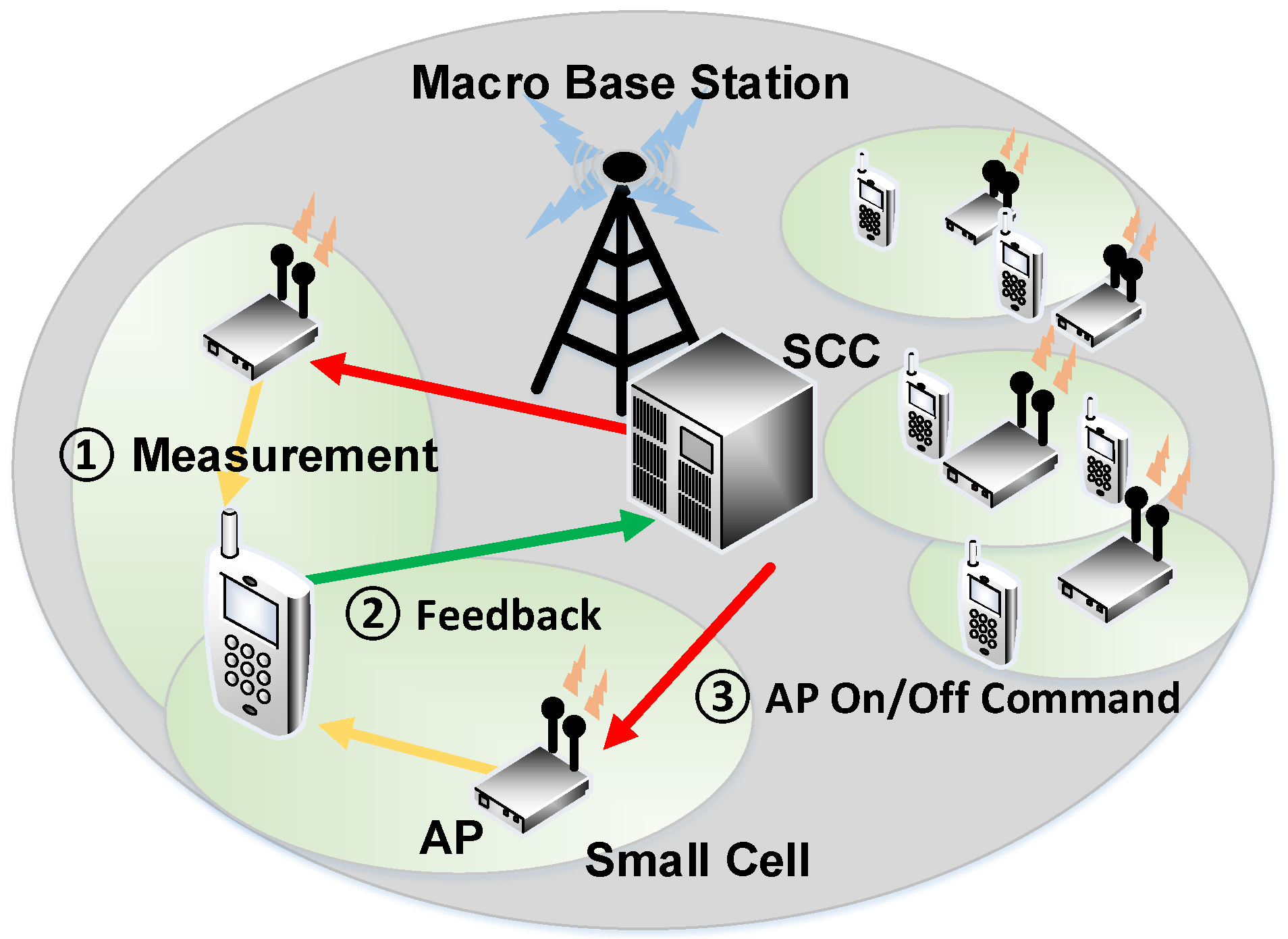
We assume that small cells can be deployed by users or an MNO; thus, the deployment can be unplanned, and small cells are randomly deployed, resulting in a dense and possibly redundant deployment. It is plausible that if the APs are placed in a home, they can use the Internet as the backhaul to communicate with the macro base station. We assume that APs are deployed in the coverage of a macro BS. For example, in NTTDOCOMO’s phantom cell concept [19], the control plane and user plane are separated in different frequency bands in which high capacity and good mobility can be supported. We assume that the control plane and the user plane are provided by the macro BS and small APs, respectively. We introduce an entity located in the macro BS called the small cell controller (SCC). From [2], the AP on/off operation can be classified into two cases: the core network (CN) controlling and UE controlling. By taking advantage of CN and UE controlling, we propose a device-assisted framework shown in Figure 1. In the device-assisted framework, UEs measure beacon signals that APs broadcast and send feedback to the SCC. Then, the SCC determines the set of turned-on APs by exploiting the feedback.
To enhance energy efficiency, turning off APs is an effective solution when APs are densely deployed. While saving energy, however, it is important to maintain the acceptable level of quality of service, which is mainly determined by the data rate. Interestingly, turning off APs can also increase the data rate when APs are densely deployed because interference among APs can be mitigated by properly selecting the set of turned-off APs. In Section 6, we show that a higher or similar average data rate is achieved by using our algorithms compared to the baseline.
We assume that the set of APs is located in the macro base station coverage, and the set of UE is in the coverage provided by APs, where is the index of AP and is the index of UE.
Definition 1 (AP on/off state indication vector).
When stands for the turned-on or off state of AP , the AP on/off state indication vector is defined by:
where J is the number of APs in the set . Note that the AP state indication vector shows a possible state of each AP. Once the SCC determines the set of turned-on APs, the vector indicates whether each AP is turned on or not. Then, we define the power consumption of the APs. While the power consumption of the APs can be affected by the utilization or load levels of APs, the power consumption of APs can be approximated as a constant value since we consider small-sized APs that consume much smaller power compared to the conventional macro BSs. Moreover, considering that the power consumption of small cell BSs is mostly from the fixed power consumption and, thus, transmission power consumption is marginal, the total power consumption can be assumed to be constant; for example, according to the data sheet of a Wi-Fi AP that has a similar hardware size of a small cell AP, the Cisco Aironet 1140 Series [20] consumes 12.95 W, while its transmission power varies from 0.78 mW to 100 mW, which is less than 1% of the total power consumption. Thus, the approximately constant power consumption can be seen as a plausible assumption. Therefore, if an AP is turned on, it consumes the operational power that includes the transmission power dissipated into the air. Thus, the operational power vector of AP is where:
and the transmission power vector of AP j becomes where:
We define the association matrix that shows the user association between APs and UEs given by:
2.2. Problem Formulation
When UE i is associated with AP j, the signal-to-interference ratio (SINR) between UE i and AP j is given by:
where is the channel gain between UE i and AP j, and is the noise power. Then, the maximum spectral efficiency of UE i served by AP j is . We assume that when an AP j has multiple associated UEs, the associated UEs are scheduled in a temporally fair way or equally when sharing the frequency channel; thus, the data rate of UE i is given by:
where . Energy consumption of APs can be calculated by summing the operational power of turned-on APs. Thus, the total power consumption of the network becomes where an indicator function is
Our objective function is the energy efficiency , also called the global function given by:
Then, we define the local energy efficiency , also called the local function, which is given by . From the definition, the local function is a part of the global function that UE i yields; thus, the global function is given by:
Our problem is to find on/off state vector that maximizes the global function . Thus, our optimization problem is:
The first constraint of (4) is from determining a set of turned-on APs. The second constraint of (5) means that turned-off APs should not be associated with any UEs. The third constraint of (6) shows that all UEs should be associated with only one APs. To tackle the problem given in (3) to (6), we need to determine the set of turned-on APs, as well as the UE-AP association. While maximizing the energy efficiency in (3), some users may experience low quality of service (QoS). Therefore, although the requirement about QoS is not explicitly expressed in the constraints of the optimization problem, minimum QoS thresholds can be set in our algorithms to ensure a minimum level of QoS, as we discuss in Section 4. Note that one can solve the optimization problem for the given traffic information, but by solving the proposed problem repeatedly, it can be also possible to adaptively manage the on/off states of APs if network traffic is changed over time. Thus, we focus on solving the above problem where the notion of time is excluded. The problem is known as NP-hard, implying that it is hard to find an optimal solution in polynomial time [9]. Thus, to solve the optimization problem, an exhaustive search should be done.
In the case of small APs, APs are usually randomly deployed, which makes the BS coordination for time/frequency orthogonal transmission very challenging. This is why we focus on the simple ON/OFF operation to improve the energy efficiency of (ultra-)dense wireless networks. Note that our problem is still very challenging because the complexity of the problem is NP-hard, and in ultra-dense networks, the computational complexity increases exponentially in the number of APs. In the next section, we apply BP to our framework and find a solution that is close to the optimal performance.
3. Belief Propagation
We adapt BP to solve our optimization problem expecting that a simple, but practical algorithm can provide an approximated solution of our problem. BP originally proposed by Pearl [21] is a message-passing algorithm widely used in inference problems. BP has successfully been demonstrated in many applications, such as error-correcting codes or artificial intelligence. By using BP, the marginals of a joint probability distribution can be calculated with iterations of message passing on graphical models including Bayesian networks and Markov random fields. We specifically focus on running BP on a factor graph, which also can be readily converted into other forms of graphical models, like Bayesian networks. For details, please refer to [22], which shows a general overview of BP, and [23,24,25], which provide explanations about BP on a factor graph. The optimization method using BP was used by the authors of [26]. The authors applied BP to inter-cell interference coordination in a femtocell network to solve the problems approximately.
By using the elements of the AP on/off state indication vector, we define a set of discrete random variables . Then, can be seen as a Bernoulli random variable denoting the turned-on or turned-off state. The realizations of the random variable is denoted by as in (1). Let us use the abbreviated notation denoting . By using these definitions above, the joint probability distribution is expressed in a shorter form .
To define the joint probability distribution , the concept of Boltzmann’s law in thermal equilibrium from statistical mechanics is used. Our framework can be seen as a system that is assumed to have J particles, and a state of each particle is denoted by . By substituting the negative of free energy part of Boltzmann’s law into our global function, is defined as:
where z is a normalization constant and τ denotes the temperature. Also, by changing the exponential of sum to product of exponentials, can be shown as
when BP is applied to the non-physical system, the temperature can be seen as a constant parameter appropriately chosen.
3.1. Factor Graph
Observing (7) and (8), we see that (7) including the global function is factorized into the product of the local functions . Thus, (8) can be shown in a factor graph. A factor graph is a bipartite graph with vertices V and edges E. Vertices, i.e., nodes of the graph, correspond to APs and UEs. There are two kinds of nodes: the variable nodes and the factor nodes. The variable nodes representing APs, shown as circle in the graph, are referred to . The factor nodes denoting UEs, shown as the square in the graph of Figure 2, are referred to , where the local function is included. Edges mean the channels between APs and UEs. To solve our optimization problem, we exploit the constructed factor graph in BP message passing.
3.2. Belief Propagation Optimization Algorithm
Following the results of [27], when , concentrates around the maxima of , and then, we have:
where , and means the marginal expectation of the random variable . In principal, standard BP can be seen as a process to calculate the estimated marginal probability distribution with respect to the random variable . Thus, when the marginal probability distribution of is estimated, an approximated solution of the optimization problem can be found.
Definition 2 (Belief).
The belief is the estimated marginal probability distribution of with respect to .
Thus, we leverage the BP algorithm to find . On the constructed factor graph, belief messages are passed through the edges between APs and UEs. After the belief message is repeatedly passed between APs and UEs, the set of turned-on APs is determined according to the estimated marginal probability distribution. It is well known that when a factor graph is acyclic, converges to the true marginal probability distribution of with respect to [26]. However, as shown in Figure 2, the constructed factor graph usually has cycles, e.g., AP 2, UE 3, AP j, UE i, and AP 2. In this case, BP yields an approximated result; thus, we compare our simulation results with the optimal value obtained from the exhaustive search in Section 5.
Now, we present the algorithm below.
- Initialization. At time , messages for and are set to have an arbitrary distribution. For instance, we use the uniform distribution, such as:
- UE update. After the initialization, UE generates and sends the belief messages to its neighboring APs where denotes the neighbor APs of UE i. At , the message update is defined by:Therefore, when the expectation (11) is calculated over independent , , the message update can be presented bywhere for given . Furthermore, in (12) is calculated for given . Since (12) has both a sum and a product, BP is called the sum-product algorithm. Equation (12) is the product of the factor with belief messages from AP , , to UE i, marginalized over all random variables, except . To calculate , at , we assume that , . At , , , is initialized to one and incremented by the number of associated UEs where each UE is associated with AP .
- AP update. AP generates and sends the belief messages to all neighboring UE , where denotes the neighbor UEs of AP j. The message is defined by:where is the normalizing constant making . The belief message (13) is the product of the belief messages from UE , all neighboring factor nodes, except i. Then, the steps ‘UE update’ and ‘AP update’ are repeated until the number of iteration is satisfied.
- Decision-making. After finishing the iteration procedure, the estimated marginal probability distribution with respect to is finalized as:where is the normalizing constant to make as a probabilistic distribution.Then, as a final step, to describe our association rule S, we define an integer-valued function that determines the position of the j-th element when the elements of the input vector are sorted in increasing order. Then, we deliberately use the following rank-based association rule of UE i given by:where , , and η is a weighting parameter considering the tradeoff between the channel condition and the estimated marginal probability from BP. The intuition of (15) is as follows. If each UE is associated with AP j solely considering energy efficiency, then most UEs are associated with a few APs having a higher value of . High may indicate that there is a global consensus that energy efficiency can be increased when the BS j is turned on. However, connecting too many UEs to one AP can degrade the data rate, which may decrease energy efficiency. In this sense, user association cannot be determined solely relying on . Thus, we exploit to determine the user association, so each UE can decide its association along with the global perspective of and also personal perspective to preserve its service quality.Our user association rule can be seen as an extension of the convention user association rule that is based on SINR. For example, if , each UE is associated with the AP that provides the highest SINR among APs in , which is the conventional user association rule. On the other hand, if , the UE is associated with the AP j whose is the greatest. It could be possible that SCC determines η to maximize energy efficiency by using adaptive learning methods. After user association is done for all UEs, the APs with no UEs are turned off.
While the BP framework is readily well defined on many graphical models, the drawback of BP framework is its complexity, which is given by from the view point of the UE. Hence, the complexity of the BP could be a barrier to large-scale ultra-dense networks of APs and UEs. Thus, we next propose online algorithms for dense cellular networks in the next section.
4. Online Algorithm: DANCE
We propose a family of online algorithms that are inspired by the BP framework. In BP, the node having a high certainty of belief can influence the final estimated marginal probability distribution. To mimic this behavior, DANCE considers priority to the AP or UE whose impact can be great. Since the ultra-dense network (UDN) environment is considered where APs are densely deployed, DANCE is designed to operate with low computational complexity.
4.1. Feedback from UE
We assume that UEs can send feedback messages as shown in Figure 1. In the SCC, the collected feedback messages constitute the feedback matrix . The feedback message can contain merely the connectivity information when using only one bit or can have more detailed information of connectivity, such as the maximum achievable data rate or appropriate adaptive modulation and coding (AMC) when using multiple bits. Thus, has two variations: a matrix is when one-bit feedback is used, and is when N-bit feedback is used. An element of a matrix, or , means that the feedback message from UE i to AP j is either one-bit or N-bit. If a one-bit message is used, represents only the connectivity. It is assumed that connectivity exists if is greater than some threshold. If an N-bit message is used, represents the achievable data rate or the quantized level of AMC. Examples of the UE feedbacks are illustrated in Table 1. We assume that the achievable data rate can be represented by using multiple N bits. In our study, N-bit message implies the achievable data rate. A study about the number of bits considering the tradeoff between performance and feedback overhead is beyond the scope of this paper and remains as a future work. However, when comparing to the BP algorithm where the repeated message exchanging is required, the DANCE algorithms only require one-time feedback messages, which significantly suppresses overall signaling overhead.
4.2. DANCE Algorithms
DANCE solves the same problem given in (3) to (6). By using matrix-based algorithms, DANCE determines the turned-on/off APs and the user association together. Once the target AP is chosen, then the association is automatically decided on the matrix , so that the result of user association is shown on the matrix . DANCE includes three algorithms: AP-first, UE-first and the proximity-ON (Prox-ON) algorithm.
In DANCE algorithms, two main algorithms, AP-first and UE-first, are designed to choose the most influential AP or UE, respectively. Depending on the type of feedback, both AP-first and UE-first have several variations: AP-N/AP-1 and UE-N/UE-1, where the number implies the length of the feedback bits. Following the categorization, AP-first and UE-first are described in Algorithms 1 and 2, respectively.
| Algorithm 1 AP-first |
|
| Algorithm 2 UE-first |
|
The algorithm works as follows. AP-first algorithms, AP-1 or AP-N, firstly choose an AP on the matrix as previously mentioned. AP-1 algorithm chooses the AP that has the greatest number of association-possible UEs. The AP-N algorithm otherwise chooses the AP that has the greatest sum of the maximum achievable data rate or the AMC of each UE depending on whether stands for the data rate or AMC levels. Then, the chosen AP is turned on, and all UEs having connectivity with the chosen AP are associated with the chosen AP. This is repeated until all UEs are associated.
As a counterpart, UE-first algorithms, UE-1 and UE-N, consider UEs foremost. For example, in the UE-1 algorithm, we firstly find the UE having the smallest number of association-possible APs, i.e., potentially the worst case UE is considered first. Then, among the APs that can connect to the chosen UE, we select the AP where in order to minimize the number of turned-on APs. Note that UE-first is a generalization of [28] where only a single bit feedback was assumed.
The other is the proximity-ON algorithm. In this algorithm, each UE associates with the AP that provides the highest SINR, while non-selected APs are turned off. It can be seen as a basic heuristic algorithm in order to determine the set of the turned-off APs. Therefore, among DANCE algorithms, the results of the proximity-ON algorithm can provide baselines to measure performance gains of AP-first and UE-first, respectively.
4.3. Practical Implementation
The message passing procedures for both the turning off and on operation in DANCE are illustrated in Figure 3. As mentioned in Section 2, each AP periodically wakes up and broadcasts a beacon signal, and each UE senses the APs’ beacon signals. Information gathered at each UE is sent to SCC. Then, SCC runs one of the DANCE algorithms in order to make a decision for each AP’s on/off status by using the feedback information from UEs. Then, SCC broadcasts the final decision to all APs, and APs follow the direction of SCC.
5. Numerical Results
In this section, we verify the proposed algorithms through extensive simulations. We first carry out the simulation for a small number of APs and UEs and then extend it for a large-scale ultra-dense network.
5.1. BP and DANCE Algorithms for a Small-Sized Network
We assume that nine APs and 20 UEs are randomly distributed in a hexagonal cell area with a 100-m radius. The AP and UE locations are determined by following a uniform distribution [2]. From the Alcatel-Lucent device (Model 9361 home cell v2), the transmission power of the AP is 13 dBm, and the operational power of the AP is 9 W. According to the IEEE 802.16 m Evaluation Methodology Document (EMD), we use the winner model assuming the non-line-of-sight (NLOS) case and propagation through light walls with a 2.1-GHz carrier frequency. The total bandwidth is 20 MHz, and the power spectral density of thermal noise is −174 dBm/Hz. Our numerical simulations are performed by taking snap shots about possible AP/UE dense deployment scenarios. This approach is also popular; see [12,29,30]. One may want to perform network-level simulations to observe packet-level behaviors, such as packet loss, related with network protocols. In this paper, however, we focus on physical-layer performance metrics, such as data rate and power consumption, to compute energy efficiency, which are in our objective function in (3).
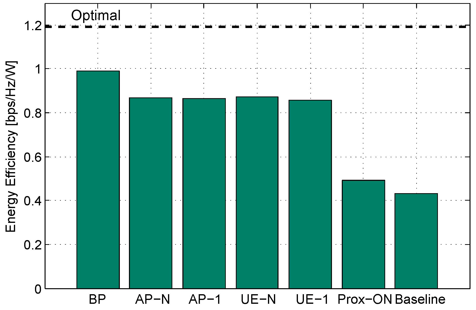
Figure 4 shows the average energy efficiency obtained through 200 iterations, and the results are summarized in Table 2. For every iteration of the proposed BP algorithm, UE update and AP update are repeated five times where and . The baseline is the case when all APs are turned on. In addition, proximity-ON is a simple heuristic algorithm, and thus, it can provide performance guidelines for other DANCE algorithms, such as AP-first and UE-first. Furthermore, we find the optimal solution by using exhaustive search. Therefore, it can be possible to compare our algorithms’ results to the case that maximizes energy efficiency.
First, we compare the average energy efficiency among BP, DANCE and the baseline in Figure 4. Table 2 represents the improvement of the average energy efficiency. Results show that BP and DANCE increase energy efficiency significantly, e.g., by 129% compared to the baseline. As expected, BP exhibits better energy efficiency than DANCE. However, the gap is not substantial, and considering that DANCE is a low complexity algorithm, the performance of DANCE is noticeable. Overall, all four cases of DANCE (AP-N, AP-1, UE-N, UE-1) achieve more or less 100% improved energy efficiency and outperform proximity-ON and the baseline substantially. In Figure 5, we compare the average power consumption and the average data rate, which are averaged over all iterations. Considering that the nature of the problem is indeed a combinatorial optimization, we compare our algorithms with an optimal solution by performing an exhaustive search. The result shows that the proposed algorithms are near optimal, e.g., achieving 83% of the optimal performance. We observe that BP and DANCE consume substantially less power than the average power consumption of the baseline. However, as the trade-off of BP’s significant power reduction, it achieves a lower average data rate. By contrast, DANCE achieves similar or even higher average data rate, which is close to the optimal energy efficiency case because the interference is mitigated by the AP off operation, and the set of turned-on APs is well chosen to provide a high data rate.
Energy efficiency, power consumption and data rate can vary with respect to η. As shown in Figure 6a, energy efficiency is maximized when . In Figure 6b, average power consumption decreases as η increases. Similarly, we observe from Figure 6c that the average data rate also decreases as η increases. This is because when η is high, the UE is associated with a small number of APs having a high value of . Then, only a small number of APs is turned on and provides connectivity for all UEs, so the overall power consumption is decreased. However, since only a few APs operate, the data rate becomes low. As a result, the desired high energy efficiency can be achieved at some proper value of η. Note that in Figure 5, as , the BP moves from the current star-marked position (★) where energy efficiency is maximized () to the position of proximity-ON (⋄). That is because proximity-ON is a special case of BP when . Thus, η is a network operator’s design parameter considering energy efficiency, power consumption and the data rate.
5.2. Expanding BP and DANCE Algorithms on UDN
From now on, we perform a large-scale simulation for UDN. Even though DANCE can be applied without any modification, the BP algorithm proposed in Section 3 needs to overcome computational complexity, and thus, we slightly modify the algorithm as follows. Instead of using a complete bipartite graph, we construct an approximated factor graph in which each UE only considers the limited number of neighboring APs. For instance, APs satisfying or , which means UE i can access AP j, are considered as neighbor APs of UE i. By doing so, each UE can have a smaller number of neighbors than the factor graph in Figure 2. The simulation results show the performance of the network in terms of the energy efficiency, UE data rate and average power consumption for the different number of APs and UEs.
5.2.1. Dense Network
Figure 7 shows the results in the case of 50 UEs where the number of APs varies from two to 100 in the hexagonal area with a radius of 158 m, so that the density of UEs, i.e., the number of UEs per , remains the same as the small-sized network in Section 5.1. As can be seen in Figure 7a, the energy efficiency of BP and DANCE is highly improved compared with the baseline. The energy efficiency of the baseline mainly decreases in the number of APs because power consumption is proportional to the number of APs. However, BP and DANCE successfully restrict the number of turned-on APs and consume lower power resulting in higher energy efficiency. For example, BP achieves five-times and AP/UE N-bit achieves nine-times higher energy efficiency than that of the baseline for the case of 100 APs. Note that, unlike the case of the small-sized network, AP/UE N-bit shows better energy efficiency than BP because BP uses the approximated factor graph. Consequently, the energy efficiency of BP increases in the practical number of APs, but has a peak around 10 APs and then decreases. However, note that the data rate of BP is the highest until 20 APs. As easily expected, the energy efficiency of proximity-ON is not very good, and that of the baseline is poor.
Remark 1 (Comparison within DANCE).
Recall that AP/UE N-bit and one-bit show almost the same energy efficiency and data rate in a small-sized network in Figure 4 and Figure 5. Now, we compare them again in a dense network. As can be seen in Figure 7c, AP/UE N-bit, as well as AP/UE one-bit both exhibit low power consumption, which is because a small number of APs are on; see Figure 7d. However, data rates are very different; while AP/UE one-bit achieves the lowest data rate among DANCE, AP/UE N-bit shows a much higher data rate, which is even comparable to those of BP, proximity-ON and the baseline. For example, the data rate of UE N-bit is 64.8% higher than UE one-bit, and the data rate of AP N-bit is 103.2% higher than AP one-bit in the case of 100 APs. Consequently, this makes AP/UE N-bit achieve higher energy efficiency than all other algorithms. Furthermore, it is interesting to observe that AP/UE N-bit show steadily increasing energy efficiency in the number of APs unlike other algorithms.
5.2.2. Ultra-Dense Network
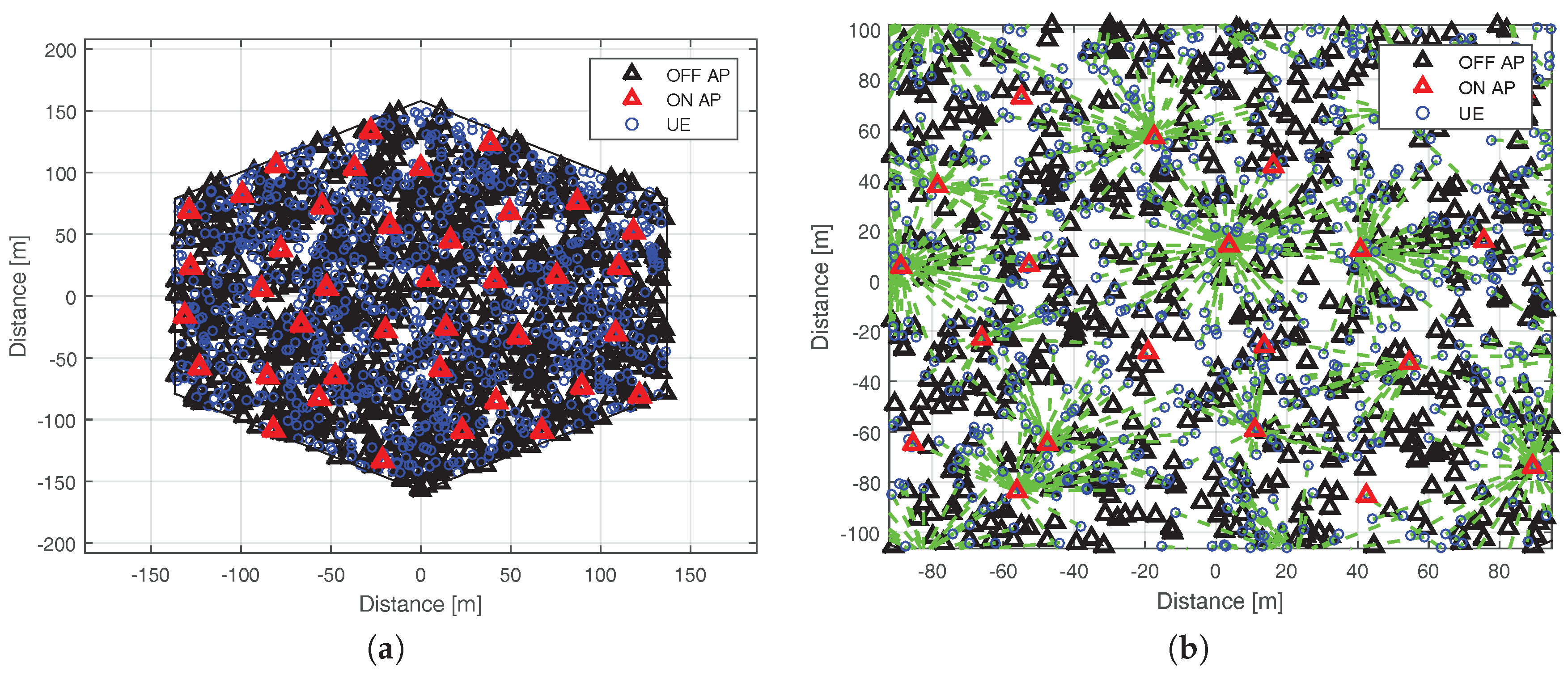
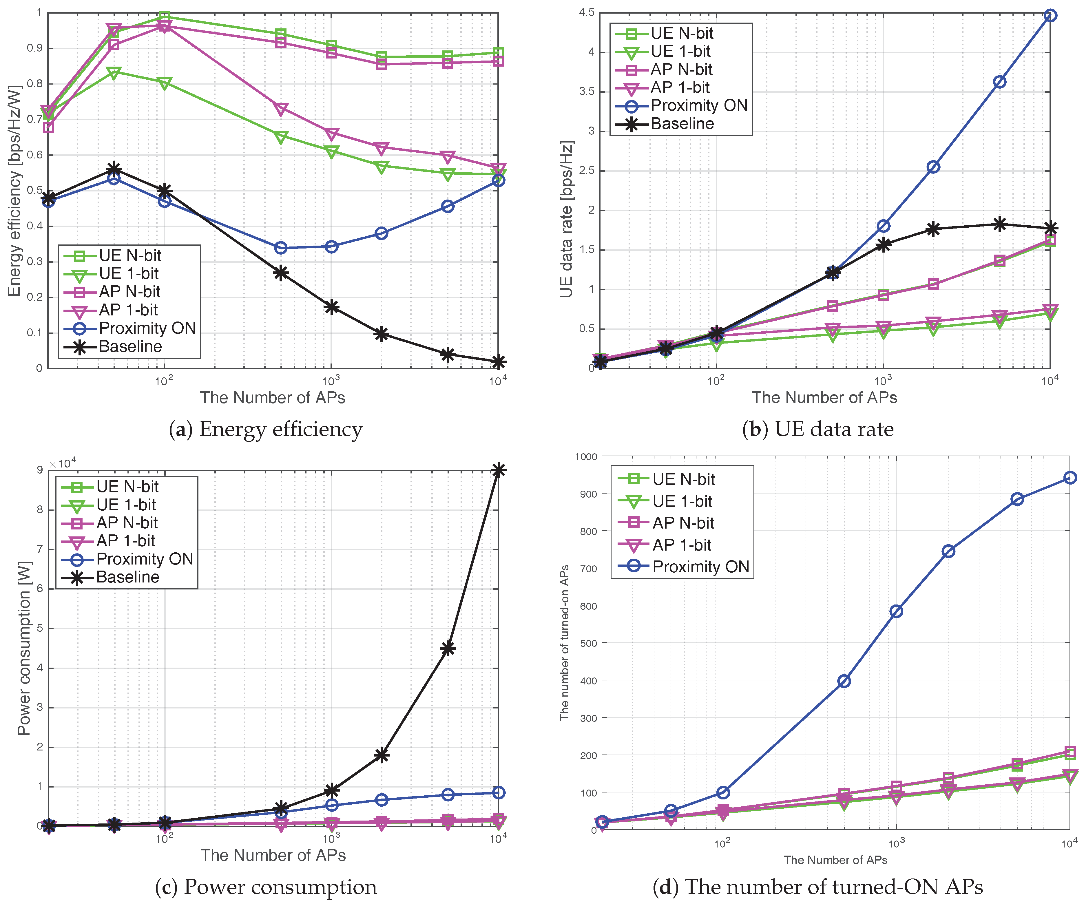
Next, we further densify both the UEs and APs; there are 1000 UE in the same area, and we vary the number of APs from 20 to 10,000, which is up to a 100-times densification. In Figure 8, the on/off state of 1000 APs is illustrated when proximity-ON is used in the case of 1000 UEs. Figure 8 shows the associations between UEs and APs. Each UE can be associated with an adequate AP, which is determined by the proposed algorithms. The APs that do not have the associated UE are turned off. Since we consider the ultra-dense deployment scenario, a UE can find the AP to be associated with, and thus, no coverage hole exists. It should be noted that this densification is extreme and may not be practical because UE needs to send out feedback for each beacon signal from each AP. Nevertheless, we investigate this case to to better understand the proposed algorithms and see how much performance gain DANCE algorithms would achieve in the extreme case. In this case, it is computationally infeasible to run BP because each UE has too many neighboring APs, even if the approximated factor graph is used. Thus, we only consider the DANCE algorithms. Other parameters are the same as in Section 5.1.
As can be seen in Figure 9, densification results in a higher data rate, but severe interference plays a role as densification goes on, specifically for the case of the baseline. We observe that the energy efficiency and data rate both grow rapidly in the low densification region, e.g., 100 APs or less. The benefit of densification in this region is well illustrated; a small increase of AP density brings the advantage of an increased data rate that outweighs the disadvantage of the increased power consumption. In addition to the baseline, one can compare the proposed algorithms with another type of baseline; since [28] corresponds to UE-1, one can see that UE-N can increase the energy efficiency up to 62.5% over that of [28] in Figure 9a.
The energy efficiency gap between the baseline and proximity-ON implies that the AP on/off operation should be enforced to enhance energy efficiency. The gap gradually enlarges when the number of APs is more than 500, which implies that even the simplest DANCE algorithm, i.e., proximity-ON, can increase energy efficiency. Note that since all APs are turned on in the baseline, high interference among APs degenerates the data rate when the number of APs approaches 5000. This also yields very poor energy efficiency. However, even under extreme densification, the energy efficiency of DANCE is highly improved in all regions. For example, in the case of 10,000 APs, UE N-bit achieves 44-times higher energy efficiency than the baseline. Specifically, Figure 9c show that UE-N and AP-N keep power consumption lower by orders of magnitude compared to the baseline. Nevertheless, Figure 9a shows that AP/UE N-bit maintains high energy efficiency even when the number of APs is more than 2000, i.e., the density of APs is very high, such as 0.0308 APs/m. In this region, although energy efficiency remains constant, the data rate of AP/UE N-bit keeps growing, implying the fraction of turned-on APs is still very low. Thus, by turning off unnecessary APs, DANCE can reduce power consumption and also achieves a high data rate thanks to effectively mitigated interference.
Remark 2 (The impact of device assistance).
Now, we discuss the impact of feedback on energy efficiency in UDN. In Figure 9a, the energy efficiency of both N-bit and one-bit feedback sharply increases for 20 APs to 100 APs (low densification region). Then, the energy efficiency of N-bit feedback is almost maintained, whereas the energy efficiency of one-bit feedback is decreased after 100 APs (high densification region). This implies that the turning off operation itself is more important to enhance energy efficiency in low densification region; without knowing detailed information, energy efficiency grows by only exploiting connectivity information embedded in one-bit feedback. However, as densification goes on, energy efficiency of one-bit feedback shrinks and eventually approaches that of proximity-ON. This indicates that we need more detailed information, including not only connectivity, but also the achievable data rate that is dynamically changed in UDN.
Remark 3 (Ultra densification and DANCE).
Deploying more APs generally provides a higher data rate; however, more power consumption is required, resulting in low energy efficiency unless carefully managed. Hence, in designing and deploying UDN, our study can suggest guidelines about the level of AP densification considering operational purposes. As seen in Figure 9a, around 100 APs, which is equal to 0.0015 APs/m, can cover the area while maximizing energy efficiency. Nevertheless, in case a greater data rate is required even at the cost of AP deployment and power consumption, DANCE, specifically AP/UE , can provide a higher data rate while keeping energy efficiency also high. For example, by increasing APs up to 1000, the data rate becomes twice, while the energy efficiency remains almost the same, which is possible because only a small portion of APs, e.g., 10%, are effectively selected as ON by DANCE.
6. Conclusions
In this paper, we have studied the mechanisms to enhance energy efficiency in the ultra-dense small cell environment. We have formulated the energy efficiency optimization problem and solved the problem by BP. To apply BP, we have constructed a factor graph, and BP has been used to derive the estimated marginal probability. Then, according to our association rule, the set of turned-on APs has been determined. Whereas BP is an offline algorithm, we also have proposed its online version called DANCE, which is inspired by BP. Numerical simulations have confirmed that the proposed BP algorithm significantly enhances energy efficiency, and DANCE requiring low complexity achieves a close performance to BP. We also have applied BP and DANCE in UDN and showed that the proposed algorithms can significantly increase energy efficiency. In UDN, BP and DANCE commonly have increased energy efficiency, e.g., up to 44-times greater than that of the baseline, but also showed different properties about the power consumption and data rate. With BP and DANCE, MNOs can achieve high energy efficiency and/or data rate by selecting one of the algorithms considering the AP and UE density and operational purposes.
Acknowledgments
This work was supported in part by the Basic Science Research Program through the National Research Foundation of Korea (NRF) funded by the Ministry of Science, ICT and Future Planning under Grant NRF-2014R1A1A1006551.
Author Contributions
Preparation of the manuscript has been performed by Gilsoo Lee and Hongseok Kim.
Conflicts of Interest
The authors declare no conflict of interest.
Abbreviations
The following abbreviations are used in this manuscript:
| AP | access point |
| UE | user equipment |
| BP | belief propagation |
| BS | base station |
| MNO | mobile network operator |
| EE | energy efficiency |
| SE | spectral efficiency |
| DANCE | Device Assisted Networking for Cellular grEening |
| SCC | small cell controller |
| CN | core network |
| QoS | quality of service |
| SINR | signal-to-interference ratio |
| UDN | ultra dense network |
| AMC | adaptive modulation and coding |
References
- Hwang, I.; Song, B.; Soliman, S.S. A holistic view on hyper-dense heterogeneous and small cell networks. IEEE Commun. Mag. 2013, 51, 20–27. [Google Scholar] [CrossRef]
- Ashraf, I.; Boccardi, F.; Ho, L. Sleep mode techniques for small cell deployments. IEEE Commun. Mag. 2011, 49, 72–79. [Google Scholar] [CrossRef]
- Fettweis, G.; Zimmermann, E. ICT Energy Consumption-Trends and Challenges. In Proceedings of the 11th International Symposium on Wireless Personal Multimedia Communications, Lapland, Finland, 8–11 September 2008; Volume 2, p. 6.
- Oh, E.; Krishnamachari, B.; Liu, X.; Niu, Z. Toward dynamic energy-efficient operation of cellular network infrastructure. IEEE Commun. Mag. 2011, 49, 56–61. [Google Scholar] [CrossRef]
- Hasan, Z.; Boostanimehr, H.; Bhargava, V.K. Green cellular networks: A survey, some research issues and challenges. IEEE Commun. Surv. Tutor. 2011, 13, 524–540. [Google Scholar] [CrossRef]
- I, C.L.; Rowell, C.; Han, S.; Xu, Z.; Li, G.; Pan, Z. Toward Green and Soft: A 5G Perspective. IEEE Commun. Mag. 2014, 52, 66–73. [Google Scholar] [CrossRef]
- Chang, C.Y.; Liao, W.; Hsieh, H.Y.; Shiu, D.S. On Optimal Cell Activation for Coverage Preservation in Green Cellular Networks. IEEE Trans. Mob. Comput. 2014, 13, 2580–2591. [Google Scholar] [CrossRef]
- Niu, Z.; Wu, Y.; Gong, J.; Yang, Z. Cell zooming for cost-efficient green cellular networks. IEEE Commun. Mag. 2010, 48, 74–79. [Google Scholar] [CrossRef]
- Son, K.; Kim, H.; Yi, Y.; Krishnamachari, B. Base Station Operation and User Association Mechanisms for Energy-Delay Tradeoffs in Green Cellular Networks. IEEE J. Sel. Areas Commun. 2010, 29, 1525–1536. [Google Scholar] [CrossRef]
- Lee, G.; Kim, H.; Kim, Y.T.; Kim, B.H. Delaunay Triangulation Based Green Base Station Operation for Self Organizing Network. In Proceedings of the IEEE Green Computing and Communications (GreenCom), Beijing, China, 20–23 August 2013; pp. 1–6.
- Moon, S.; Kim, H.; Yi, Y. BRUTE: Energy-efficient user association in cellular networks from Population Game Perspective. IEEE Trans. Wirel. Commun. 2015, 15, 663–675. [Google Scholar] [CrossRef]
- Soh, Y.S.; Quek, T.Q.; Kountouris, M.; Shin, H. Energy efficient heterogeneous cellular networks. IEEE J. Sel. Areas Commun. 2013, 31, 840–850. [Google Scholar] [CrossRef]
- Cho, S.R.; Choi, W. Energy-efficient repulsive cell activation for heterogeneous cellular networks. IEEE J. Sel. Areas Commun. 2013, 31, 870–882. [Google Scholar] [CrossRef]
- Peng, J.; Hong, P.; Xue, K. Energy-Aware Cellular Deployment Strategy under Coverage Performance Constraints. IEEE Trans. Wirel. Commun. 2014, 14, 69–80. [Google Scholar] [CrossRef]
- Wang, Z.; Zhang, W. A Separation Architecture for Achieving Energy-Efficient Cellular Networking. IEEE Trans. Wirel. Commun. 2014, 13, 3113–3123. [Google Scholar] [CrossRef]
- Cao, P.; Liu, W.; Thompson, J.S.; Yang, C.; Jorswieck, E.A. Semidynamic Green Resource Management in Downlink Heterogeneous Networks by Group Sparse Power Control. IEEE J. Sel. Areas Commun. 2016, 34, 1250–1266. [Google Scholar] [CrossRef]
- Wu, J.; Zhang, Y.; Zukerman, M.; Yung, E.K.N. Energy-Efficient Base-Stations Sleep-Mode Techniques in Green Cellular Networks: A Survey. IEEE Commun. Surv. Tutor. 2015, 17, 803–826. [Google Scholar] [CrossRef]
- Lee, G.; Kim, H. Green Small Cell Operation Using Belief Propagation in Wireless Networks. In Proceedings of the IEEE Globecom Workshops, Austin, TX, USA, 8–12 December 2014; pp. 1266–1271.
- Nakamura, T.; Nagata, S.; Benjebbour, A.; Kishiyama, Y.; Hai, T.; Xiaodong, S.; Ning, Y.; Nan, L. Trends in small cell enhancements in LTE advanced. IEEE Commun. Mag. 2013, 51, 98–105. [Google Scholar] [CrossRef]
- Cisco. Cisco Aironet 1140 Series Access Point Data Sheet. Available online: http://www.cisco.com/c/en/us/products/collateral/wireless/aironet-1130-ag-series/datasheet_c78-502793.html (accessed on 7 December 2016).
- Pearl, J. Reverend Bayes on Inference Engines: A Distributed Hierarchical Approach. In Proceedings of the National Conference on Artificial Intelligence (AAAI), Pittsburgh, PA, USA, 18–20 August 1982; pp. 133–136.
- Yedidia, J.S.; Freeman, W.T.; Weiss, Y. Understanding belief propagation and its generalizations. Explor. Artif. Intell. New Millenn. 2003, 8, 236–239. [Google Scholar]
- Kschischang, F.R.; Frey, B.J.; Loeliger, H.A. Factor graphs and the sum-product algorithm. IEEE Trans. Inf. Theory 2001, 47, 498–519. [Google Scholar] [CrossRef]
- Frey, B.J.; Kschischang, F.R.; Loeliger, H.A.; Wiberg, N. Factor Graphs and Algorithms. In Proceedings of the Allerton Conference on Communication, Control, and Computing, Monticello, IL, USA, 28–30 September 1997; Volume 35, pp. 666–680.
- Yedidia, J.S.; Freeman, W.T.; Weiss, Y. Constructing free-energy approximations and generalized belief propagation algorithms. IEEE Trans. Inf. Theory 2005, 51, 2282–2312. [Google Scholar] [CrossRef]
- Rangan, S.; Madan, R. Belief propagation methods for inter-cell interference coordination in femtocell networks. IEEE J. Sel. Areas Commun. 2012, 30, 631–640. [Google Scholar] [CrossRef]
- Dembo, A.; Zeitouni, O. Large Deviations Techniques and Applications; Springer: Berlin/Heidelberg, Germany, 1998. [Google Scholar]
- Vereecken, W.; Deruyck, M.; Colle, D.; Joseph, W.; Pickavet, M.; Martens, L.; Demeester, P. Evaluation of the potential for energy saving in macrocell and femtocell networks using a heuristic introducing sleep modes in base stations. EURASIP J. Wirel. Commun. Netw. 2012, 2012, 1–14. [Google Scholar] [CrossRef] [Green Version]
- Weng, X.; Cao, D.; Niu, Z. Energy-Efficient Cellular Network Planning under Insufficient Cell Zooming. In Proceedings of the 73rd Vehicular Technology Conference (VTC Spring), Budapest, Hungary, 15–18 May 2011.
- Oh, E.; Son, K.; Krishnamachari, B. Dynamic Base Station Switching-on/off Strategies for Green Cellular Networks. IEEE Trans. Wirel. Commun. 2013, 12, 2116–2136. [Google Scholar] [CrossRef]
Figure 1.
System model of the green small cell operation assisted by devices.

Figure 2.
Example of a factor graph consisting of variable nodes, AP j, , and factor nodes, UE i, .
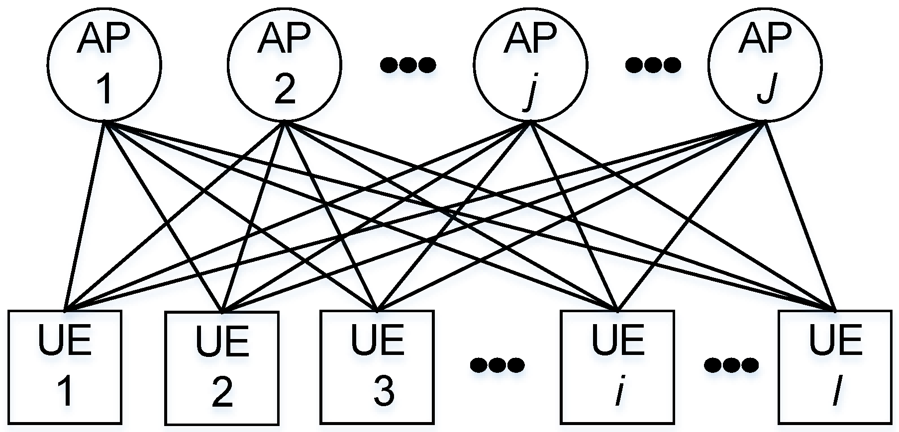
Figure 3.
Green small cell operation and procedure using the DANCE algorithm.
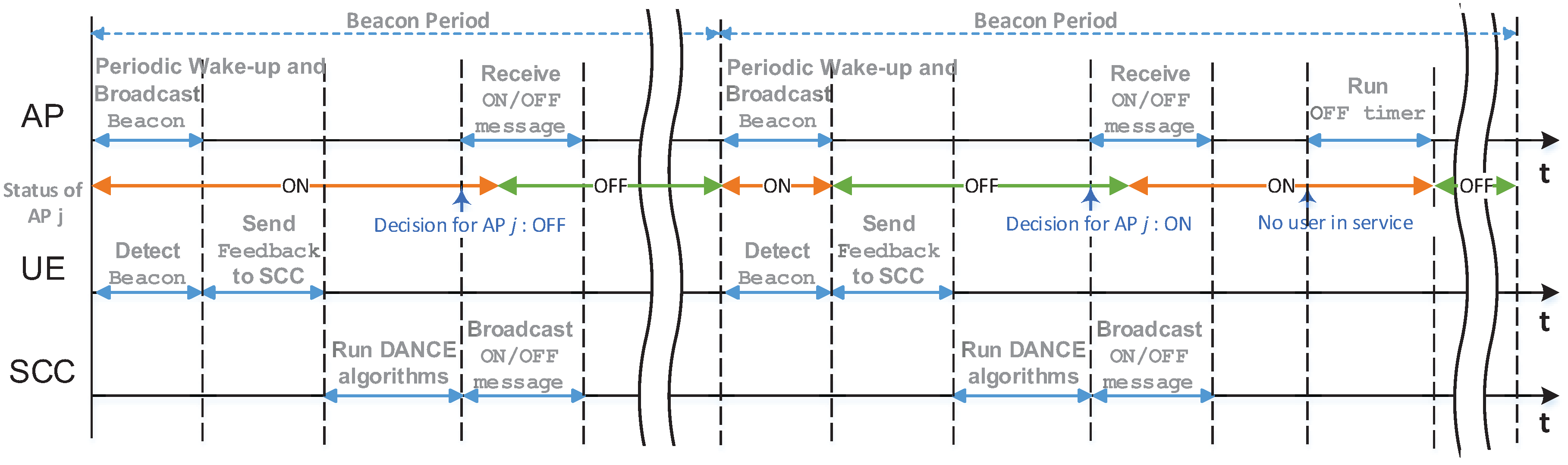
Figure 4.
Comparison of the average energy efficiency among BP, DANCE and the baseline.

Figure 5.
The average power consumption vs. the average data rate.
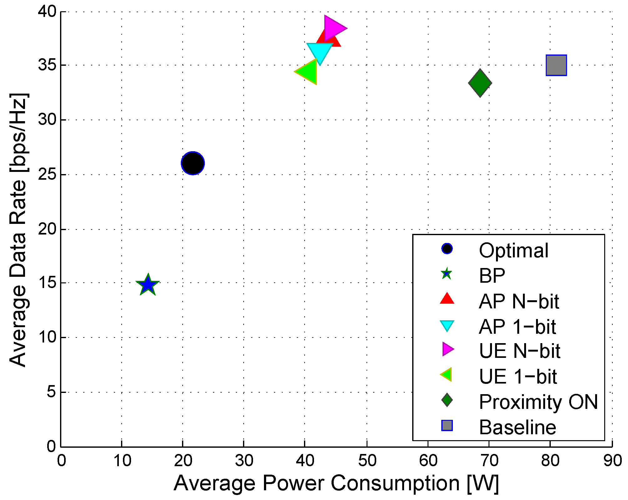
Figure 6.
The average energy efficiency, power consumption and throughput with different values of η. (a) Average energy efficiency; (b) average power consumption; (c) average data rate.
Figure 6.
The average energy efficiency, power consumption and throughput with different values of η. (a) Average energy efficiency; (b) average power consumption; (c) average data rate.
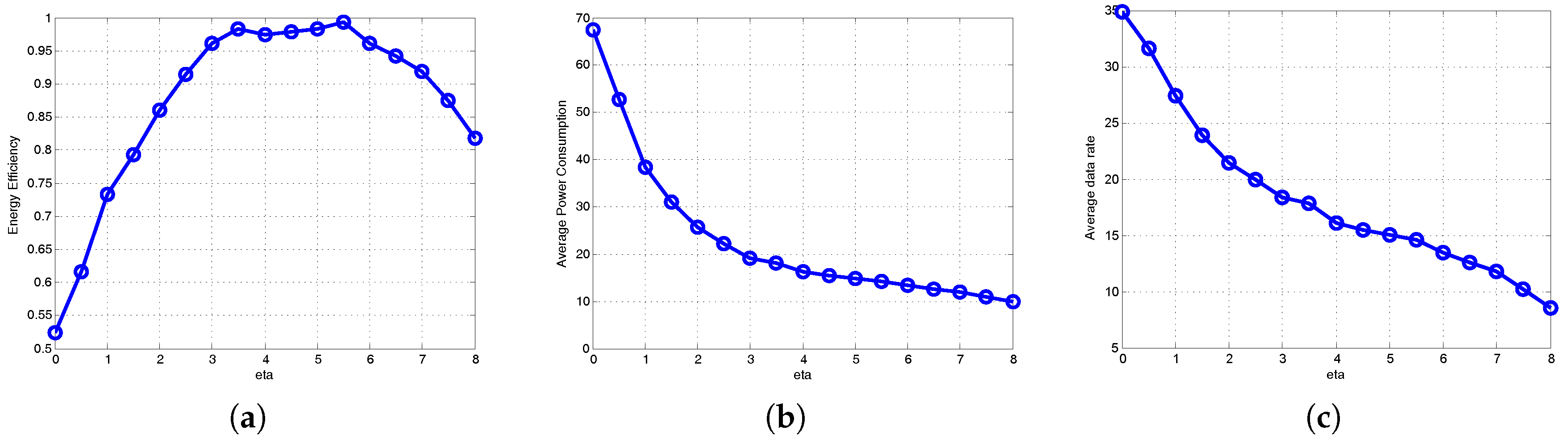
Figure 7.
Green small cell operation under dense networks.
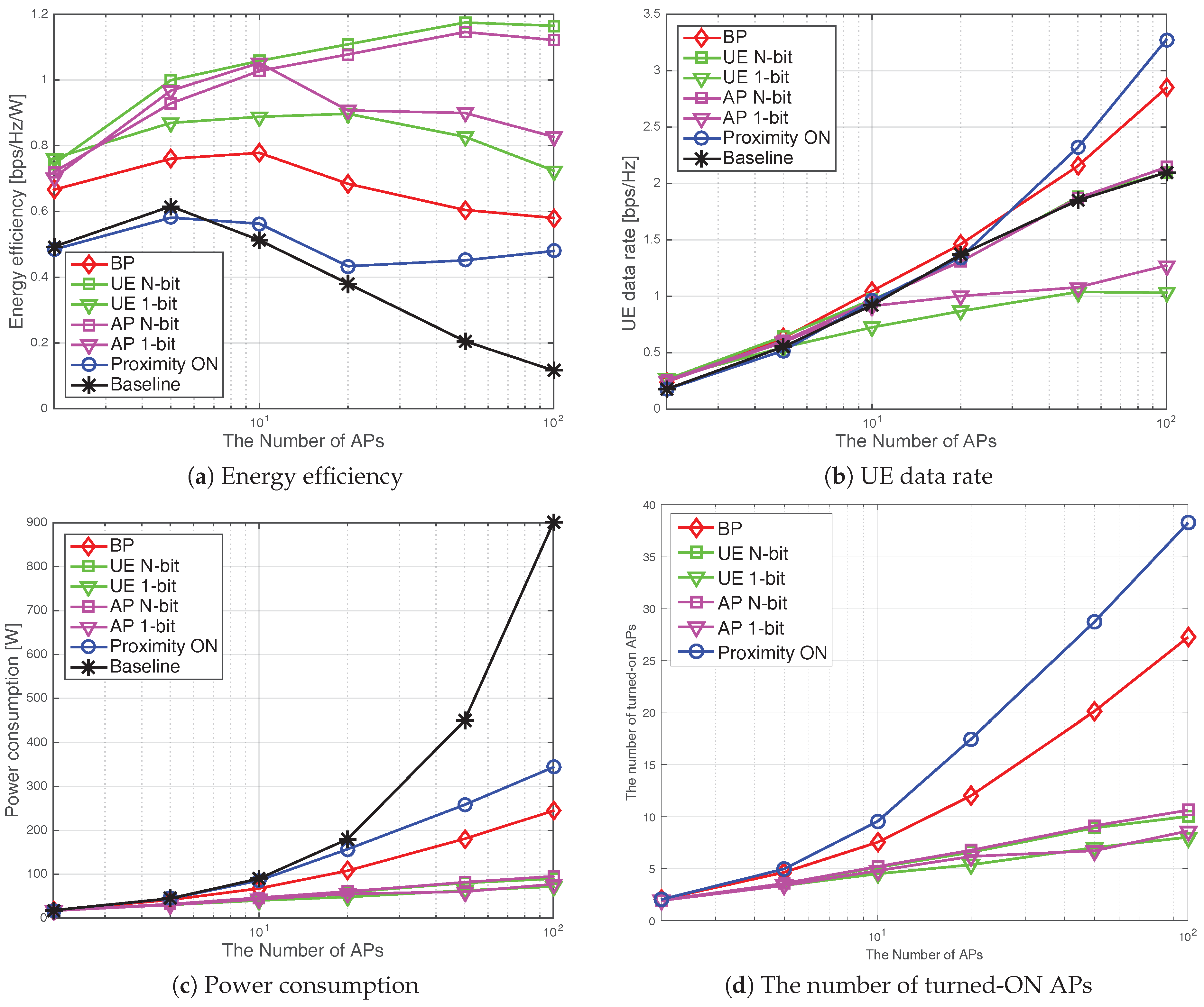
Figure 8.
An example of the ON/OFF states of 1000 APs when the UE-N algorithm is used in the case of 1000 UEs. (a) Thirty nine APs turned on among 1000 APs; (b) user association between turned-ON APs and UEs.
Figure 8.
An example of the ON/OFF states of 1000 APs when the UE-N algorithm is used in the case of 1000 UEs. (a) Thirty nine APs turned on among 1000 APs; (b) user association between turned-ON APs and UEs.

Figure 9.
Green small cell operation under ultra-dense networks.


| 1-bit Feedback () | N-bit Feedback () | Association Matrix (S) |
|---|---|---|
Table 2.
The average energy efficiency improvement percentages of the proposed algorithms to the baseline. Prox-ON, proximity-ON.
| BP | AP-N | AP-1 | UE-N | UE-1 | Prox-ON |
|---|---|---|---|---|---|
| 129% | 101% | 100% | 102% | 98% | 14% |
© 2016 by the authors; licensee MDPI, Basel, Switzerland. This article is an open access article distributed under the terms and conditions of the Creative Commons Attribution (CC-BY) license (http://creativecommons.org/licenses/by/4.0/).
Share and Cite
MDPI and ACS Style
Lee, G.; Kim, H. Green Small Cell Operation of Ultra-Dense Networks Using Device Assistance. Energies 2016, 9, 1065. https://doi.org/10.3390/en9121065
AMA Style
Lee G, Kim H. Green Small Cell Operation of Ultra-Dense Networks Using Device Assistance. Energies. 2016; 9(12):1065. https://doi.org/10.3390/en9121065
Chicago/Turabian StyleLee, Gilsoo, and Hongseok Kim. 2016. "Green Small Cell Operation of Ultra-Dense Networks Using Device Assistance" Energies 9, no. 12: 1065. https://doi.org/10.3390/en9121065
Note that from the first issue of 2016, this journal uses article numbers instead of page numbers. See further details here.