HVDC-System-Interaction Assessment through Line-Flow Change-Distribution Factor and Transient-Stability Analysis at Planning Stage

Abstract

Many of the recent projects for new transmission line have considered the high-voltage direct current (HVDC) system, owing to the many advantages of the direct current (DC) system. The most noteworthy advantage is that a cable can serve as a substitute for the overhead transmission line in residential areas; therefore, the HVDC system application is increasing, and as the number of DC systems in the power system increases, the interaction assessment regarding the HVDC system gains importance. An index named multi-infeed interaction factor (MIIF) is commonly used to estimate the interaction between power converters; however, the HVDC system is composed of two converters and a transmission line. The MIIF represents the interaction between the rectifiers and inverters, but not for the whole system. In this work, a method to assess the interaction of the whole system was therefore studied. To decide on the location of the new HVDC transmission system at the planning stage, in consideration of the interaction of the existing DC system, the line flow change distribution factor, according to the HVDC-transmission capacity change, was examined. Also, a power system transient -stability analysis was performed with different HVDC system locations, depending on the distribution factor. The simulation results indicate that when the factor is higher, two HVDC systems have a stronger interaction and are less stable in the transient state.

1. Introduction

The high-voltage direct current (HVDC) system has been used since 1954 [1,2,3]. After the introduction of the first direct current (DC) transmission system, many of the current operators of the HVDC systems, as well as organizers of new transmission line projects, have considered DC transmission, as DC systems have more advantages [4]. The most important advantages are as follows:

• Interconnection between power systems with different frequencies, or asynchronous systems
• Environmental benefits regarding right-of-way width, radio interference, and underground cables
• Power transmission over hundreds of miles
• Transmission-power control

Among those advantages, the most noteworthy feature is that a cable is available as a substitute for overhead transmission lines. The consideration of DC systems is also because new transmission line construction is becoming more difficult due to environmental issues and low degrees of residents’ acceptance; in such cases, underground cables can avoid these problems. In Korea, new construction of ultra-high voltage (UHV) alternating current (AC) transmission lines are still delayed or have been cancelled due to residents’ reluctance; therefore, high-capacity HVDC systems are being considered for the transmission of power from generation sites to load areas, while underground cables will be used in residential areas.

Also, the HVDC system’s application is increasing in terms of renewable energy interconnection. Renewable energy generation sites, such as offshore wind farms, are usually far from main systems, and they have asynchronous frequencies. So, the HVDC system is suitable for interconnection between renewable generation sites and main power systems.

Direct current transmission is also installed to establish connections from large-scale generation areas to metropolitan areas. The capacity of devices based on power electronics is increasing rapidly due to the development of power electronics technology and increases in HVDC-rated power. Also, large-scale generation plants are usually far from residential areas, which are load-centralized areas. Further, DC has an advantage over AC in terms of long-distance transmissions, so it is used in cases of long-distance connections between generation sites and load areas.

The growth of HVDC system penetration can cause problems that are different from those of single-infeed HVDC converters [5,6]. A commutation failure can occur due to the different behavior and stability of voltage or power based on different features of the single-infeed HVDC system [7,8,9]; therefore, the interactions between multiple HVDC systems in an AC system need to be estimated to reduce the negative effects, and to operate the system normally. The interaction between power converters is usually assessed by multi-infeed interaction factor (MIIF) [10]. According to Davies et al., who proposed this index, the most reflective parameter of the interaction is the inverter AC bus voltage. The MIIF represents the interaction between two converters’ AC voltages. The MIIF is used in the HVDC planning stage when the AC system strength is calculated. In the HVDC planning stage, the AC system strength is considered through the effective short circuit ratio (ESCR) for the single-infeed HVDC; however, the multi-infeed effective short circuit ratio (MIESCR) is calculated for the multi-infeed HVDC.

The MIIF and MIESCR are indices for which the converter interaction is considered, and the value of the indices is determined based on the electrical distances between the inverters or the rectifiers. Because the rectifier and inverter are evaluated individually, the index cannot consider the whole system at once.

In this work, a method that assesses the interaction between HVDC systems was studied. The existing interaction assessment is focused on the voltage relationship. However, the parameter changed by fluctuation in the state of the power system is not only the voltage, but all of the parameters, which change concurrently. System state fluctuation causes voltage and current changes and, consequently, the line flow changes when a disturbance occurs. The line flow is related to the sending and receiving of the end voltage, and the current is calculated using the voltages and the line impedance. Assuming that the AC transmission line at the location of the new HVDC is installed, the line-flow change that occurs when the existing HVDC flow changes can be used as an index to evaluate the interaction sensitivity of the location. The change represents the electrical relation between the locations of two HVDC systems. We calculated the line-flow distribution factor and performed a simulation to verify that the line-flow change is associated with the interaction. We also performed a dynamic simulation using different distribution factors to estimate the transient stability.

2. Voltage Interaction

2.1. Multi-Infeed Interaction Factor

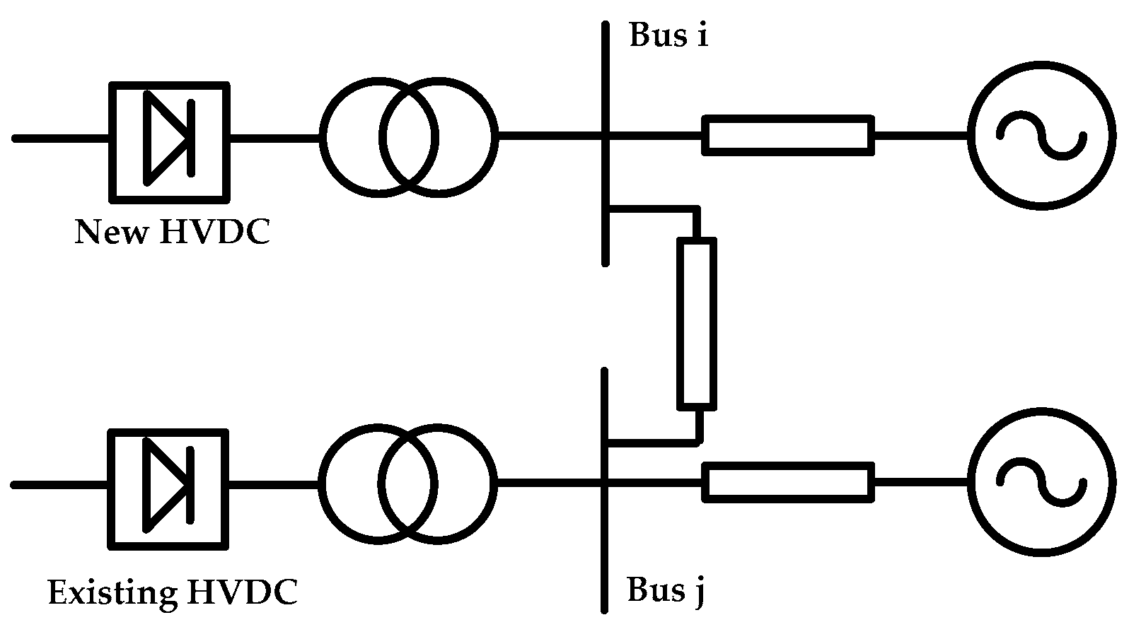
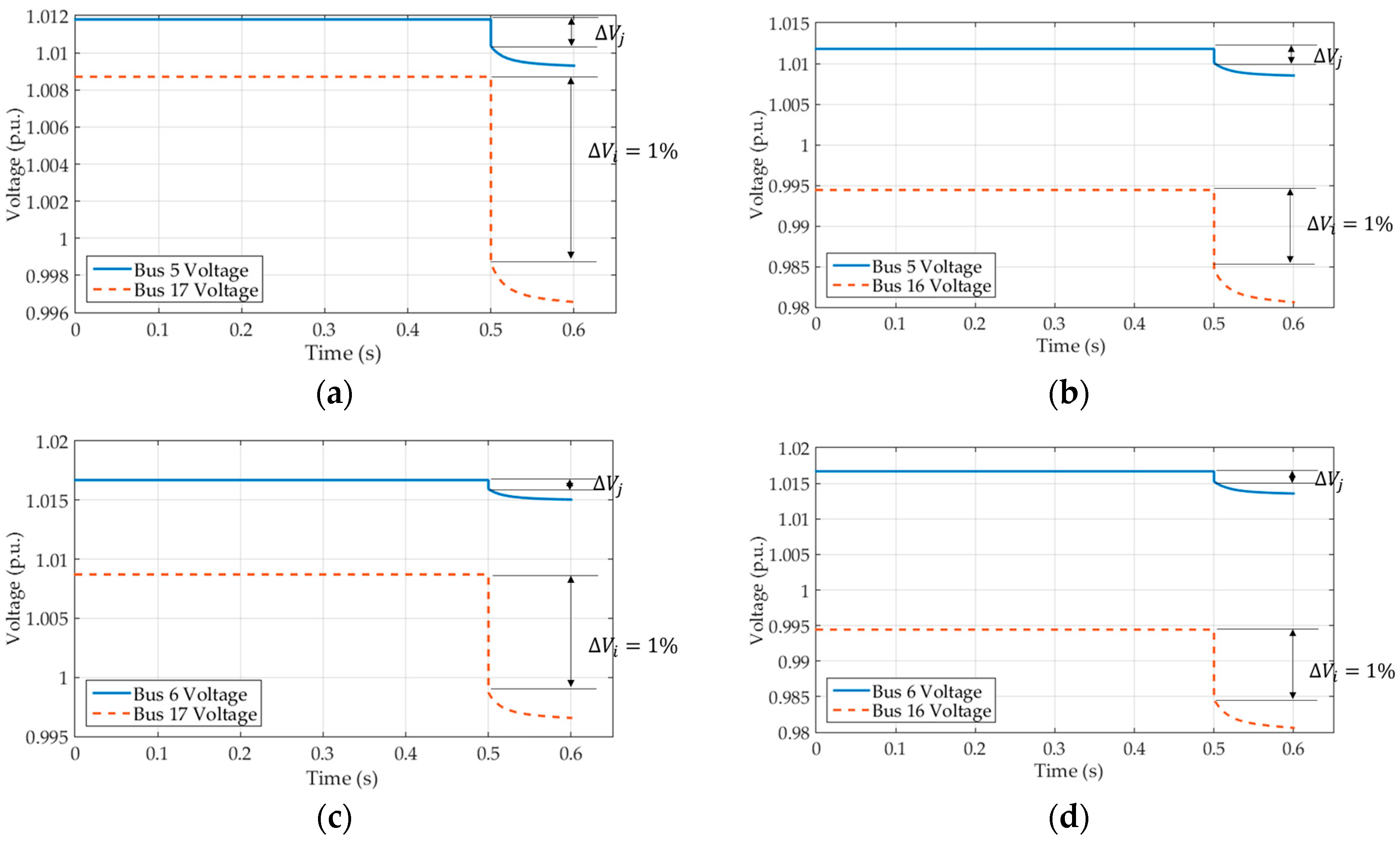
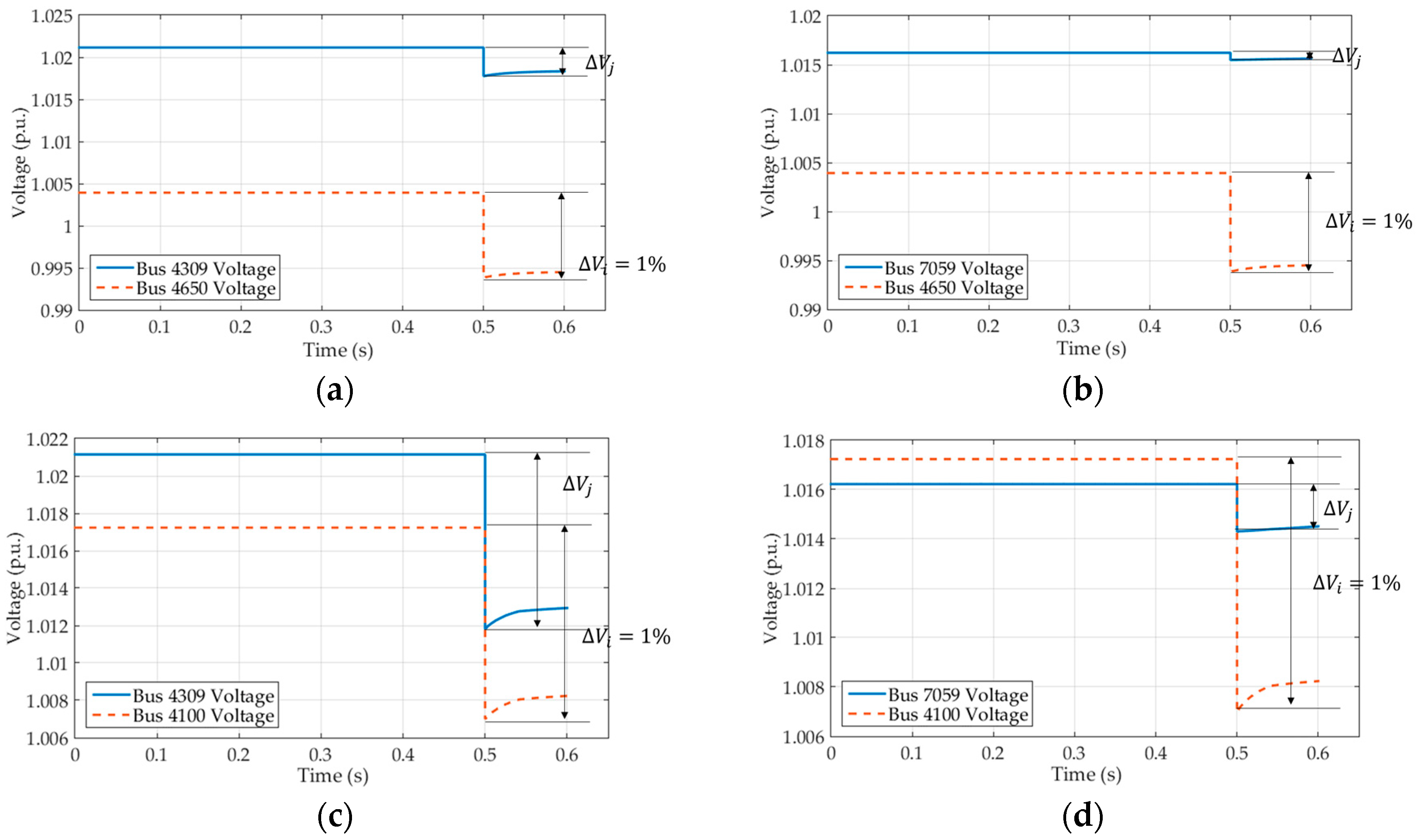
The new HVDC is connected to the AC bus i, and the existing HVDC is connected to the AC bus j, as shown in Figure 1. The MIIF is the voltage change of the bus j over the voltage change of bus i, and the value of the voltage change for bus i is the recommended 1% change.

$$MII{F}_{i,j}=\frac{\Delta V_j}{\Delta V_i}$$

(1)

Equation (1) represents the mathematically defined MIIF. When the voltage change $\Delta V_i$ is 1%, the voltage change ratio of bus j is the MIIF. If bus i and bus j are located electrically far apart, the value of the MIIF will approach zero. As the value is increased, the closer the electrical distance between the two buses becomes, so the value approaches 1. If two converters are located at the same bus, the MIIF will be 1. There are three methods to obtain the value of the index [11]. The methods are as follows:

• Dynamic simulation
• Network admittance calculation
• Fault current calculation

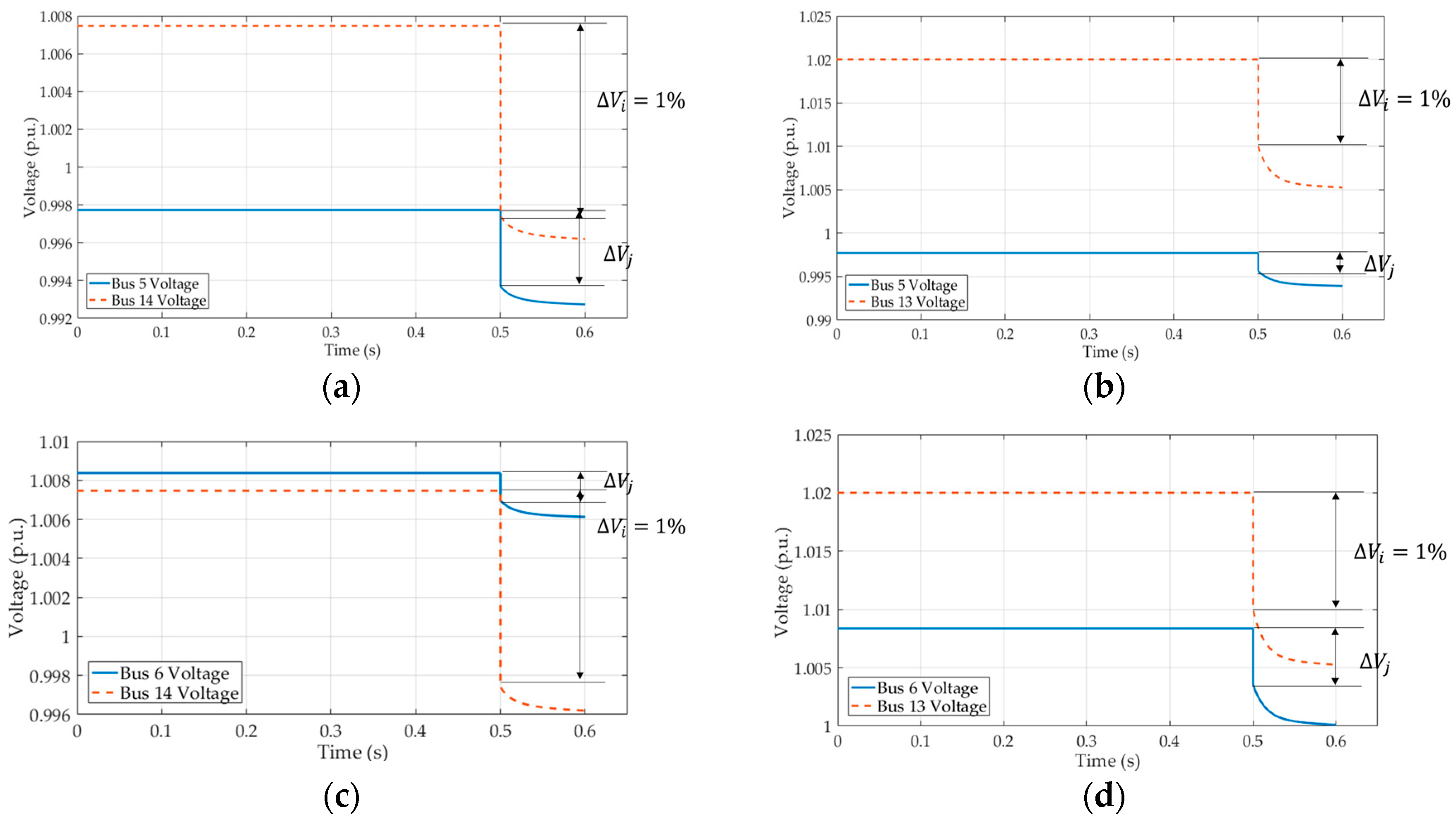
The network admittance calculation method is not recommended, owing to a large number of computations. The impedance matrix should be calculated here, which is the inverse matrix of the admittance matrix. The Y-bus matrix would be very large for a large network, and then the calculation of the Z-bus matrix is difficult because of problems such as singularity and computation burden. The dynamic simulation method and fault current calculation method are verified through a sample case study in this paper. The notations of MIIF used in this paper are MIIF1 (II), MIIF2 (IR), MIIF (RI), and MIIF4 (RR). MIIF1 (II) and MIIF4 (RR) means MIIF between inverters (II) or rectifiers (RR). MIIF2 represents the interaction between the inverter of the new HVDC and the rectifier of the existing HVDC (IR) or the rectifier of the new HVDC and the inverter of the existing HVDC (RI).

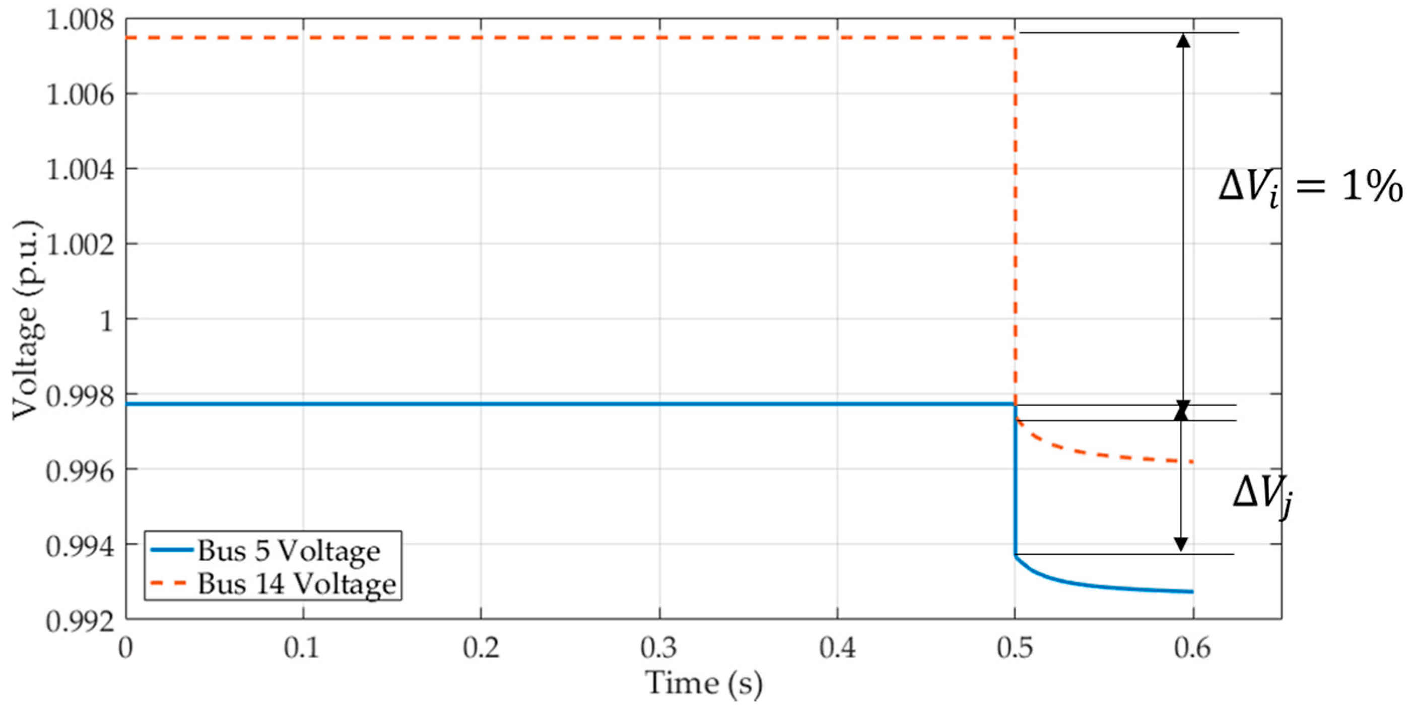
A sample case of the MIIF is studied next, and Figure 2 represents the result. The test system is modeled in the dynamic simulation program PSS/E, and the fault is applied during the simulation. The MIIF value between the two inverters for the test system is 0.4041.

Table 1. MIIF calculation by fault current method.

Bus	Actual Fault Current (kA)	Fault Current (p.u.)
Fault at bus i	8.3217	0.701
Fault at bus j	9.376	0.790
Fault at both bus	11.8719	1.0
$MII{F}_{i,j}$	0.4647
$MII{F}_{j,i}$	0.5236

shows result of MIIF calculation by fault current method and fault current in per unit (p.u.) means fault current value divided by fault current at both bus. The MIIF calculated by the fault current method is 0.4647, which is approximately 15% different from that of the dynamic simulation method; therefore, even though the fault calculation method is valid for determining the MIIF value without a dynamic simulation, the value is different from that of the dynamic simulation method. The dynamic simulation method is therefore used in the simulation described in this paper because the method is commonly used to calculate the MIIF.

2.2. Multi-Infeed Effective Short Circuit Ratio

The short circuit ratio (SCR) is an index that indicates the AC system strength, which is significant for the HVDC system performance [12]. Also, the effective SCR (ESCR) is an index for the calculation of the strength of an AC system for which filters and shunt capacitors, among others, are considered [13]. The ESCR is more meaningful with respect to the HVDC system performance due to a consideration of the reactive power compensation. In the planning stage, the ESCR is therefore evaluated at the converter station AC bus to verify that the AC system is strong enough to operate the HVDC system normally.

The SCR formulas are as follows:

$$SCR=\frac{\mathrm{Short}\mathrm{Circuit}\mathrm{Capacity}\left(\mathrm{MVA}\right)}{P_{DC}\mathrm{rating}\left(\mathrm{MW}\right)}$$

(2)

in which the short circuit capacity, SCC, is given as follows:

$$SC{C}_i=\frac{E_{\mathrm{AC},i}^2}{Z_{th,i}}$$

(3)

However, for the reactive power compensation, the SCR does not consider factors such as filters, shunt reactors, or capacitors. The reactive power capacity affects the equivalent of the AC system in terms of the converter bus; consequently, it affects the HVDC performance. To consider the effect of the reactive power capacity, the ESCR is used. The ESCR is given by the following:

$$ESCR=\frac{\mathrm{SCC}\left(\mathrm{MVA}\right)-{\mathrm{Q}}_f}{P_{DC}\mathrm{rating}\left(\mathrm{MW}\right)}$$

(4)

The ESCR is assessed in the case of the single-infeed HVDC system to verify that an AC system is sufficiently strong. If the calculated value is over 2.5, the system is judged as strong enough to operate the HVDC system normally. If the system has a second HVDC system, the ESCR should consider the effect of the interaction, so the MIESCR is defined as follows:

$$MIESCR=\frac{\mathrm{SCC}\left(\mathrm{MVA}\right)-{\mathrm{Q}}_f}{{\displaystyle \sum _{j=1}^{n}MII{F}_{i,j}\times P_{DC}}}$$

(5)

The rated capacity of the existing HVDC is multiplied by the MIIF, and the values are considered with the new HVDC-rated capacity when the AC system strength is evaluated; therefore, the MIESCR is one of the methods for the consideration of the interaction between HVDC systems in the planning stage.

Nevertheless, there is still more research to conduct to improve the MIIF or the MIESCR because the indication is the converter interaction in regard to the voltage. Details of different types of MIESCR are explained in References [14,15,16,17]. Researchers tried to improve the MIIF, because the index was made for the evaluation of the interaction between two inverters. However, the cases where the HVDC systems are in the same AC system are increasing; therefore, studies have considered the interaction between the rectifier and inverter. A method for the assessment of the interaction of the entire HVDC system according to the electrical distance and the line flow is described in this paper.

3. Line Flow Change Distribution Factor

The HVDC system is a transmission system. Accordingly, the interaction should be evaluated in view of the transmission line. Obviously, the terminal voltages and the current of the line change due to transmission line state fluctuations. MIIF can assess terminal voltage changes, but current change is not considered. So, the current change should be observed to assess the interaction between HVDC systems. In this study, the line-flow change was observed when the existing HVDC changed its own flow to observe both voltage and current changes. The line-flow change distribution factor was defined as the difference of the active power.

However, the HVDC system line-flow is determined from the controller-power order. The current change can be observed only with respect to the AC transmission line. If the plan for the new HVDC is the replacement of the existing AC line, the line-flow change can be observed using the existing power system data, because the data has an AC line at the location of the newly planned HVDC system. However, if the plan is a new construction, the power system data may include HVDC data; therefore, the new HVDC system should be replaced by the AC line in the data to observe the flow change.

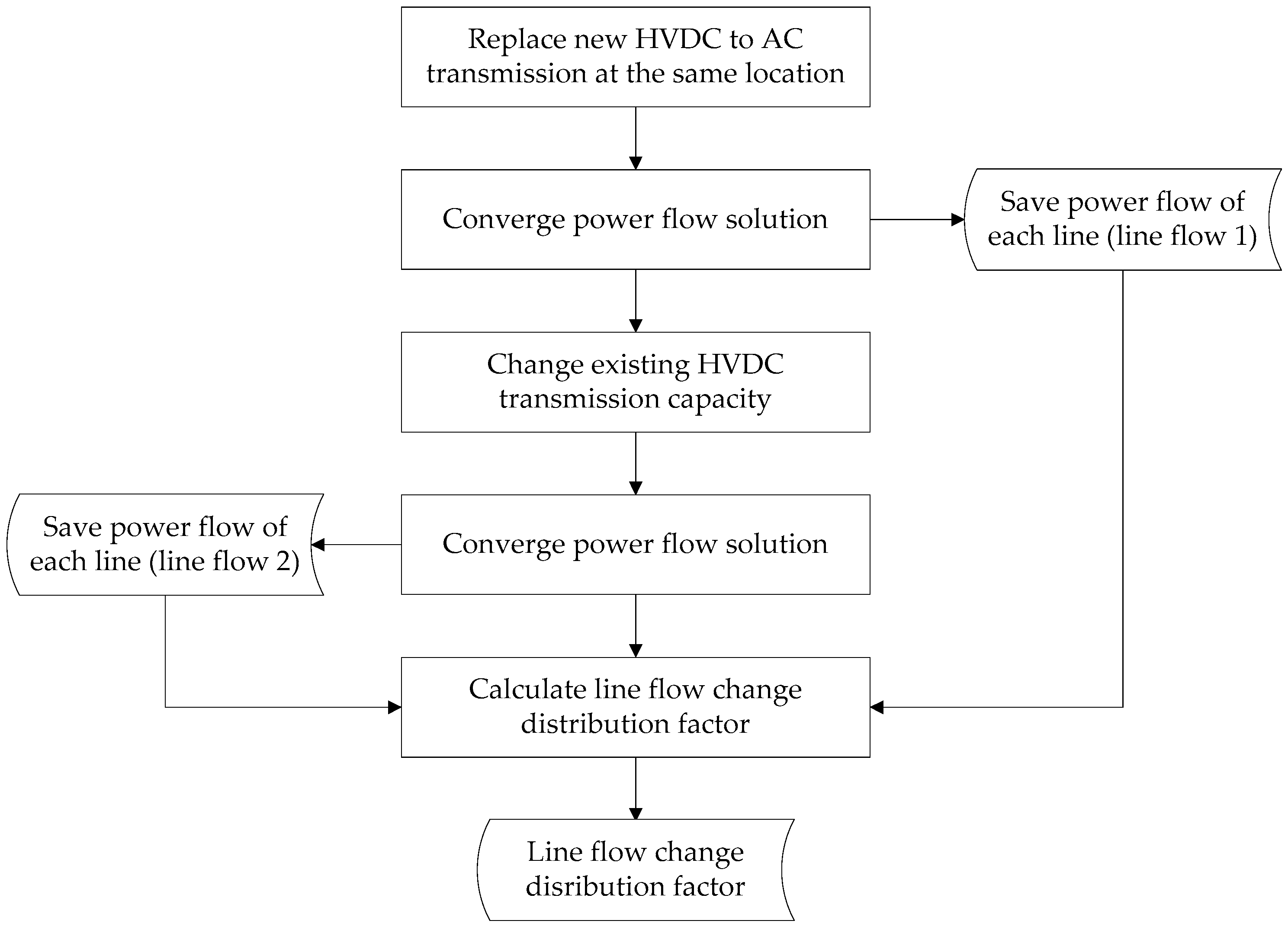
Figure 3 indicates the flowchart for the calculation of the line-flow change distribution factor. Although the voltage and current change at the line cause both active and reactive power changes, only the former was observed for the calculation of the distribution factor. Because the line-flow change occurred due to the existing HVDC active power fluctuation, the distribution factor is focused on the active power change. The line-flow change is mathematically defined as follows:

$$\mathrm{Line}\mathrm{flow}1=P_1+j{Q}_1,\mathrm{Line}\mathrm{flow}2=P_2+j{Q}_2$$

(6)

$$\mathrm{Line}\mathrm{flow}\mathrm{change}\mathrm{distribution}\mathrm{factor}=\frac{P_1-P_2}{\Delta P_{DC}}$$

(7)

Line flow 1 is the result from the first power-flow calculation, as shown in Figure 3. After the existing HVDC transmission capacity changed, the power-flow calculation derives line flow 2. The line-flow change distribution is the difference between Line flows 1 and 2 divided by the changed amount of the DC transmission. Consequently, the factor describes the distributed capacity from the total changed amount.

The line-flow change distribution factor is similar to the power transfer distribution factor (PTDF) in terms of the line-flow change that is observed [18]. The PTDF is based on the generation and load change of different zones. Nevertheless, to calculate the proposed factor, the generation capacity or load capacity is unchanged in the power system data. The existing HVDC transmission capacity is the only changed data. Also, the factor is based on the solution of the AC power flow calculation, while the PTDF is based on the DC power flow calculation.

A higher value of the factor means that the location is electrically close and the lines are detours of the existing HVDC; therefore, an interaction between the locations with a high factor value is strong. That is, if the new HVDC is installed at the location, the new device has a great effect on the existing device; alternatively, it is possible that the relatively normal operations of the new HVDC are shown when it is installed at the location of the lower distribution factor.

4. Simulation Result

4.1. Modified IEEE 39 Bus Test System

The assessment of the interaction according to the proposed factor was simulated by the power system analysis tool PSS/E, which was used to calculate the interaction factors, and the transient stability was analyzed by the same tool using the generic dynamic model of the HVDC. Modified IEEE 39-bus test system data was used to verify the effect of the line-flow change distribution factor, and the interaction according to the factor was evaluated and compared with the MIIF. The transient stability analysis was performed with the HVDC dynamic model, which is the CDC6TA. The model includes protection functions and has been proposed for studying new DC lines [19]. The protection functions of the model are blocking, bypassing, mode switching, delayed blocking, and delayed bypassing. Also, the model includes voltage-dependent current order limit (VDCOL). Therefore, unblocking, unbypassing, and VDCOL characteristics are configurable, and general values of the functions are used in the paper to characterize the HVDC system as a general HVDC system.

Figure 4 shows the modified location in the IEEE 39-bus test system. The HVDC is modeled between buses 5 and 6, and the system data is the base case of the simulation. The two candidate locations of the new HVDC were assumed. The new HVDC system location for case 1 is between bus 13 and bus 14, and case 2 has the DC system between buses 16 and 17.

The line-flow change distribution factor and MIIF were calculated for both cases, and the transient stability analysis was performed as well. The dynamic model of the new HVDC system is required to calculate the MIIF, or to perform the transient stability analysis; however, the characteristics and dynamic model of the planned HVDC system are usually not decided in the planning stage; therefore, the CDC6TA model was used with certain parameters for the modeling of the new DC system. Control mode of the new HVDC system was set as constant power control, therefore, inverter control mode is constant DC voltage and rectifier controls current to follow power order value. Current order is calculated by power order and DC voltage value. Therefore, inverter controls have a gamma angle to control DC voltage to a set value, and rectifier controls have an alpha angle to adjust current to a calculated order value.

From the results of the calculations, the factor value of case 1 is 0.3341, while the case 2 location has a lower value of 0.432. Also, the MIIF values for each converter were simulated and calculated using the dynamic simulation method. The calculation results are represented in

Table 2. Line-flow change distribution factor and MIIF calculation results for test system.

Case Number	Line-Flow Change Distribution Factor	MIIF1 (II)	MIIF2 (IR)	MIIF3 (RI)	MIIF4 (RR)
Case 1	0.3341	0.4041	0.2123	0.1435	0.4862
Case 2	0.0432	0.1479	0.1799	0.0794	0.1513

. The simulation results are represented in Figure 5 and Figure 6.

The line-flow change distribution factor is also related to the electrical distance that is in common with MIIF. But the MIIF values are different from each other. In case 1, MIIF1 and MIIF4 have bigger values than MIIF2 and MIIF3. However, the MIIF values for case 2 are lower than 15%, which are negligible except for MIIF2.

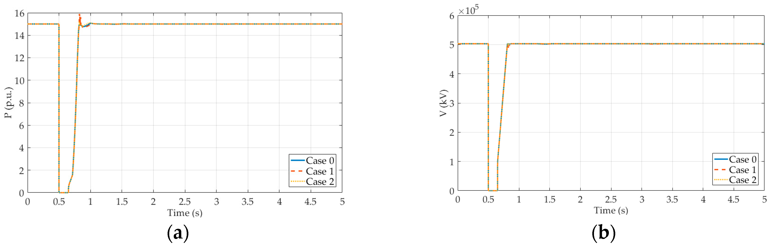
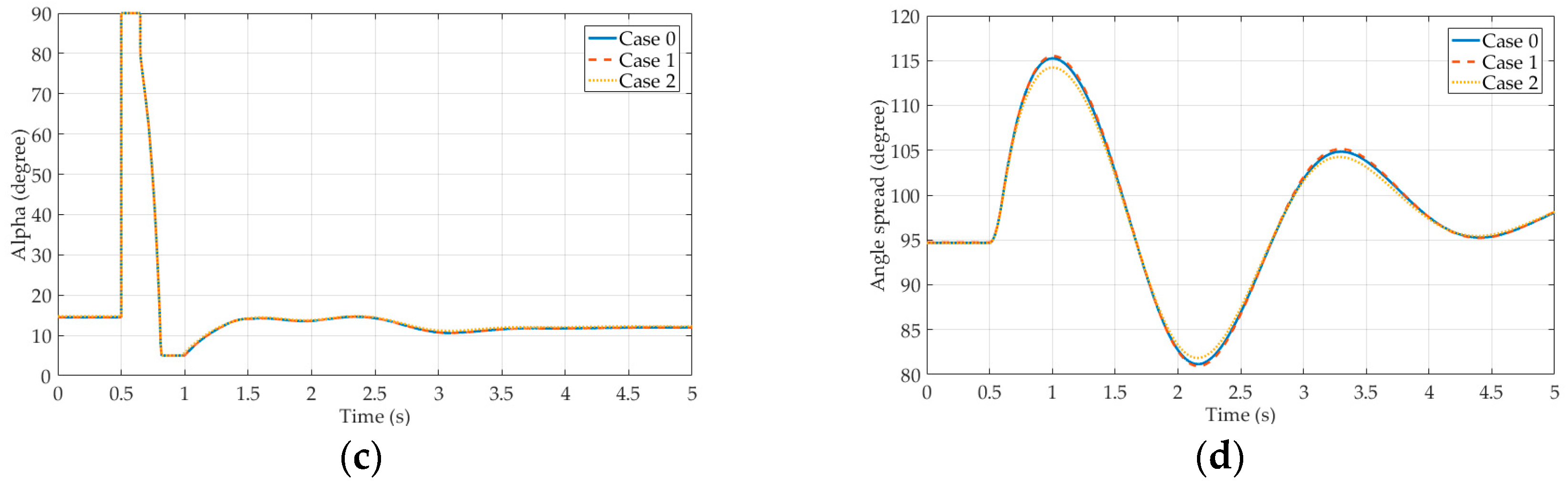
The transient stability analysis was performed and compared with the base case, which is the power system with the single-infeed HVDC. The existing HVDC performance was influenced by the new HVDC system, and the effect is stronger from the system with the higher line-distribution factor. Also, the angle spread was observed to evaluate the transient stability of the AC system. Angle spread is an index that represents the AC system’s transient stability, and it is defined as the difference between the largest and smallest machine angles in the system. If a disturbance occurs, the angle spread of the system will fluctuate and become stable after a few swings. For a stable system, the index may have a maximum value at the first swing, and the maximum value is larger for bigger disturbances; therefore, the power system can be judged as more stable when the maximum value of the angle spread is lower for the same disturbance. The maximum value is used to judge the systemic transient stability in this paper.

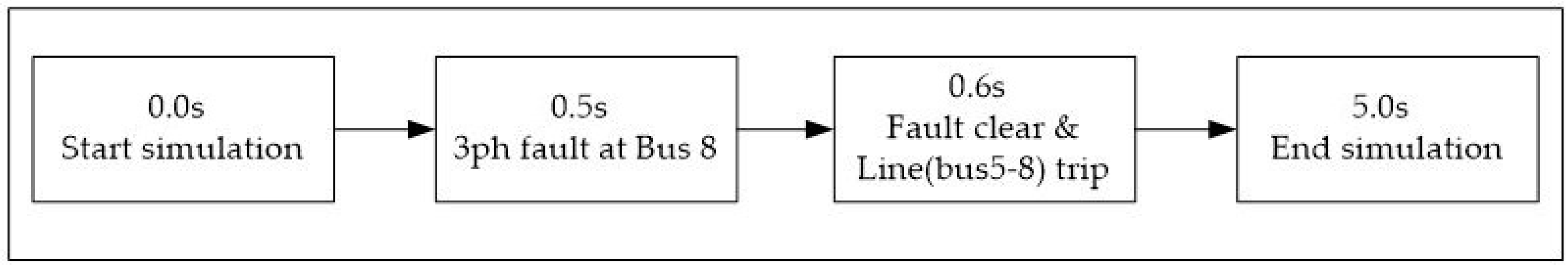
The simulation was performed with the same contingency. The contingency scenario is the 3-phase bus fault near the existing HVDC system. A detailed scenario is shown in Figure 7.

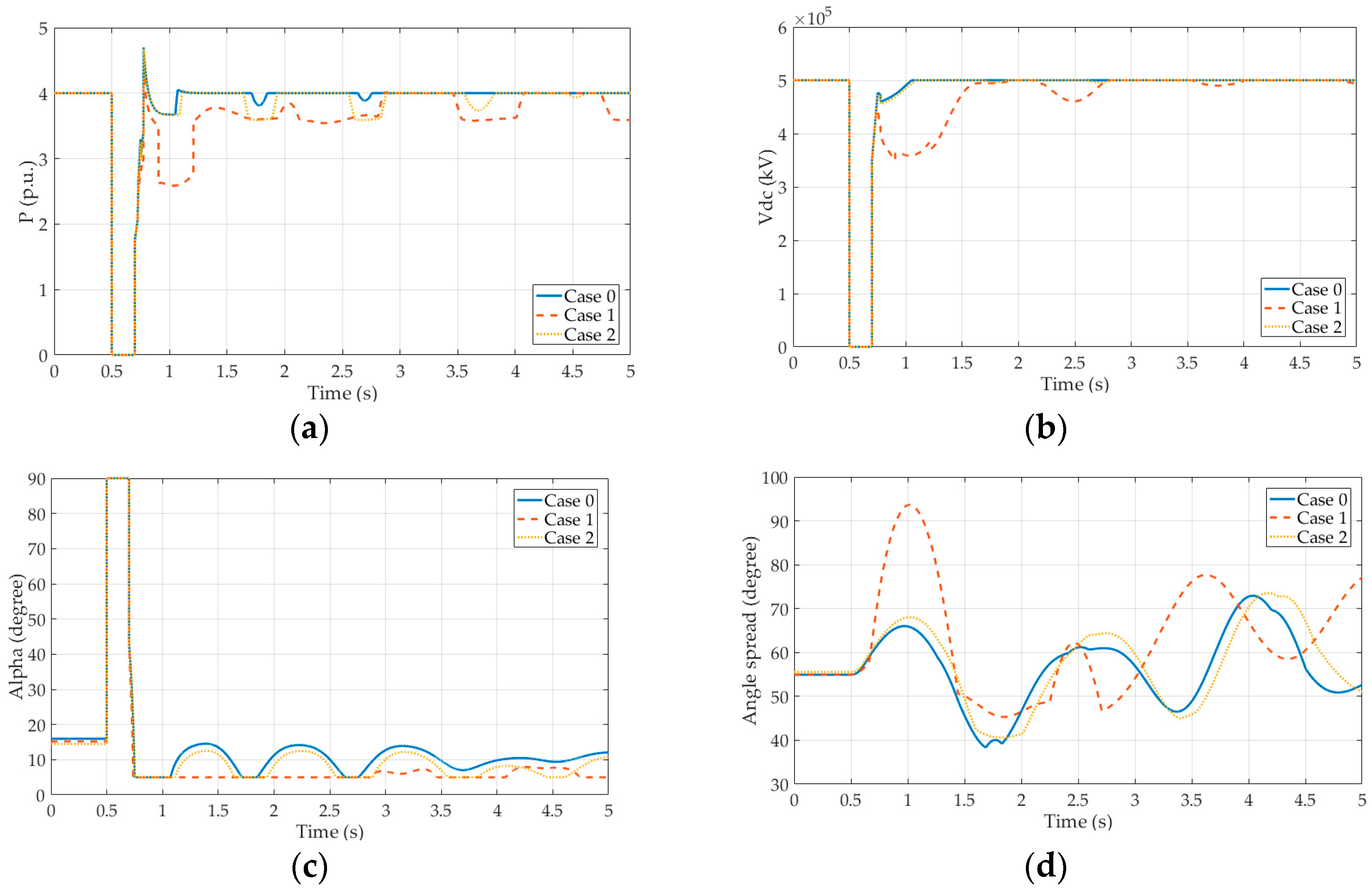
Figure 8 indicates the existing HVDC system performance for each case from the transient stability simulation result. Case 0 is the base case, which is the single-infeed case, so the existing HVDC system is the only DC system. The HVDC shows the best performance in the base case; however, case 2 has similar results for the DC voltage and alpha angle. Also, the AC system’s angle spread of case 2 is similar to that of the base case. The maximum value of the angle spread appeared at the third swing in both the base case and case 2. The maximum value of case 2 is slightly higher compared to the value of the base case.

The HVDC performance of case 1 deteriorated evidently. The DC voltage recovery feature is worse, and the alpha angle met the limit for the longer duration. As a consequence, the AC system transient stability is worse as well. These results show that case 1 had a stronger interaction between the HVDC systems, and that the interaction had a negative effect on the existing HVDC performance. The minimum MIIF of case 1 is MIIF3, which is 0.1435, and the value is smaller than MIIF2 of case 2, which is 0.1799. The MIIF has a different value according to the interaction assessment subject, so the selection of the converter for the evaluation of the interaction is important. On the contrary, the line-flow change distribution factor does not need to be selected, because the factor is determined by the location of the DC system.

4.2. Korean Power System

The test system is a relatively weak system compared with the Korean power system, so the interaction between the HVDC systems is strong. Notwithstanding whether the MIIF of case 2 is small enough, the new HVDC system had a negative effect on the system stability; therefore, the same procedure was simulated with the Korean power system’s data to verify the line-flow change distribution factor in a strong AC system.

Table 3. Line-flow change distribution factor and MIIF calculation results for Korea power system.

Case Number	Line-Flow Change Distribution Factor	MIIF1 (II)	MIIF2 (IR)	MIIF3 (RI)	MIIF4 (RR)
Case 1	0.1063	0.2051	0.3929	0.0338	0.2152
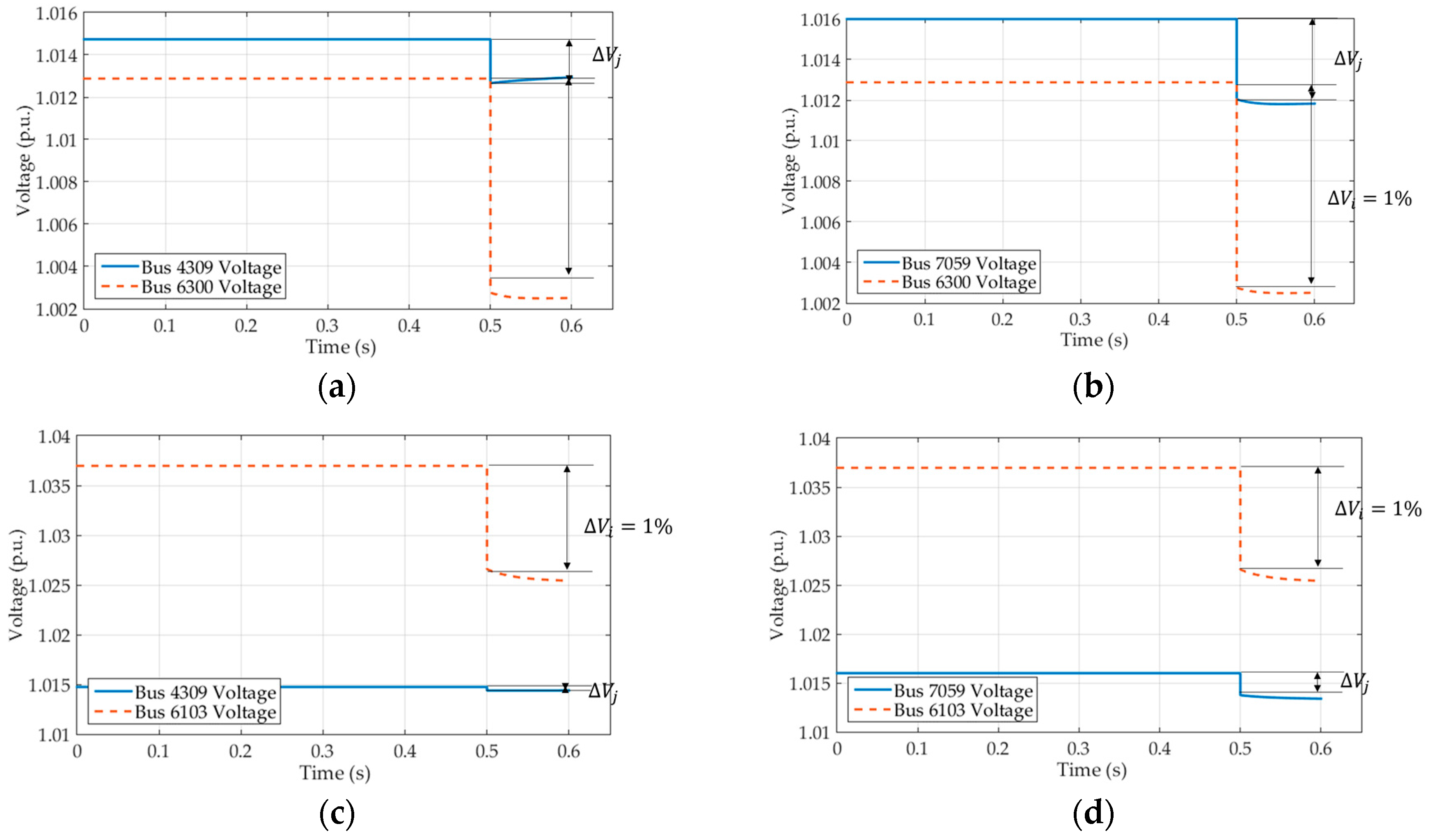
Case 2	0.0165	0.3343	0.0707	0.9110	0.1867

indicates the calculation results of the MIIF and line-flow change distribution factor for the Korean power system test data. Case 1 and case 2 each include a new HVDC system, and the interaction of the DC system with the existing HVDC system was assessed. The MIIF simulation results are shown in Figure 9 and Figure 10.

The maximum MIIF of case 1 is 0.3929 for the new HVDC inverter and the existing HVDC rectifier. The minimum value between the rectifier of the new HVDC and the inverter of the existing system is 0.0338. This value means that the electrical distance between the converters (IR) is closest in case 1; however, MIIF3 (RI) is small enough to ignore. In case 2, the maximum MIIF is MIIF1, which is 0.3343, and the value is analogous to MIIF2 for case 1. Nevertheless, the line-flow change distribution factors are significantly different. The factor is 0.1063 for case 1, while the factor for case 2 is 0.0165; that is, the line-flow change distribution factors can be certainly different even if the MIIF values are similar.

The transient simulation for the Korean power system was performed with the same scenario from the test system, but the tripped lines are two circuits. Simulation results are represented in Figure 11. The existing HVDC performance was observed and compared with that of each case, including the base case. The angle spread of the AC system was observed as well. The Korean power system is a relatively strong system, so the scenario was a small disturbance, and the effect of the interaction is weak. Consequently, the existing HVDC performance is very similar in each case, but is slightly different for case 2.

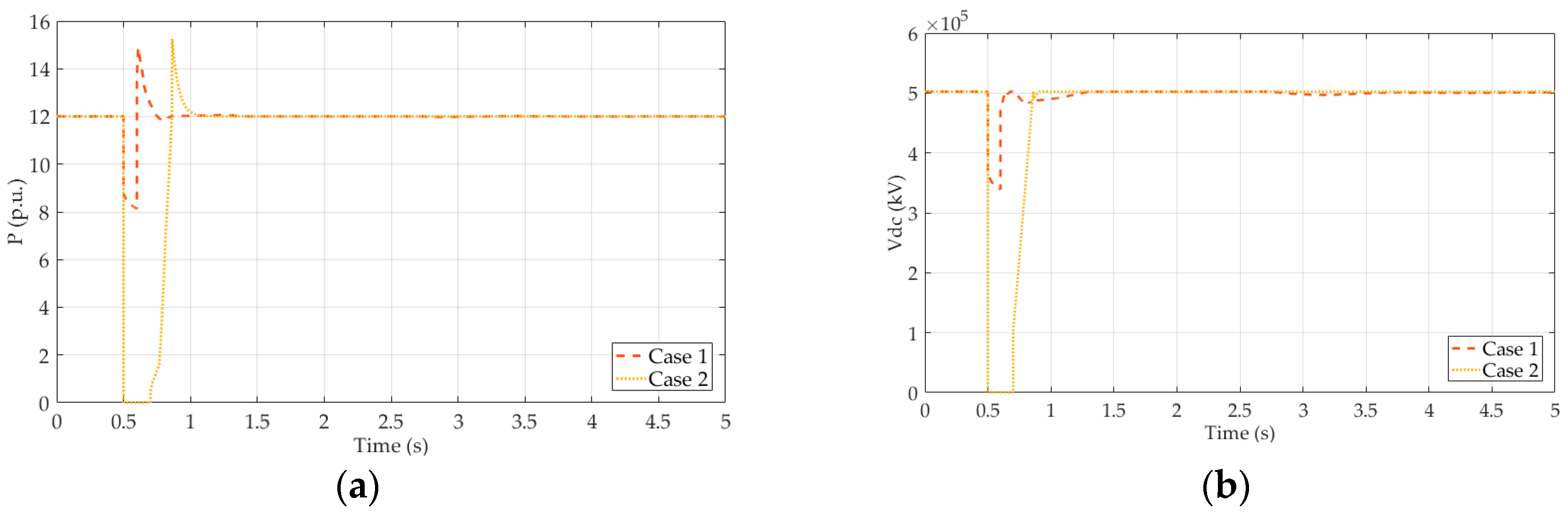
The new HVDC performance was observed as well. The HVDC performances in case 1 and case 2 are completely different due to the fault that occurred at the bus location and the AC voltage. The HVDC performance graph is represented in Figure 12. The DC system of case 2 was blocked because of the fault, but the case 1 HVDC was operated with a reduced active power transmission, while a shorter duration than the HVDC in case 2 is due to the blocked duration; therefore, the fault location had a greater effect on the new HVDC of case 2.

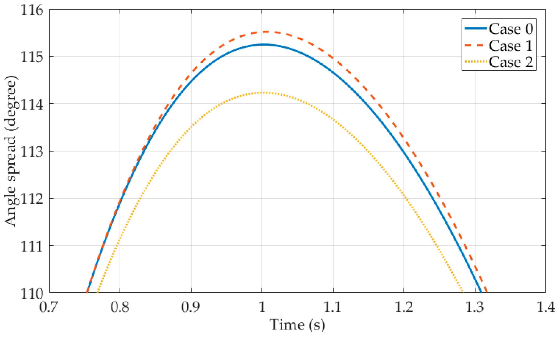
Even though the performance of the new HVDC in case 2 is worse, the transient stability of case 2 is better than that of case 1, and even for the base case. The transient stability was judged by the angle spread of the AC system in this paper. The maximum value of the angle spread appeared on the first swing. The value of case 2 is lower than that of the base case. Detailed angle spread graphs are shown in Figure 13. So, if the new HVDC is installed at a location with a low line-flow change distribution factor, the interaction between the DC systems is weak, and even the power system transient stability can be improved.

5. Conclusions

Installations of the flexible AC transmission system (FACTS), or the high-voltage direct current (HVDC) system, have recently increased in number. As the use of the DC system increases, the risk of abnormal interaction operations also increases; therefore, the interaction between devices or systems that are based on power electronics needs to be assessed to operate the system normally. There is an index named MIIF to evaluate the HVDC interaction, and the index is considered at the planning stage as MIESCR; however, the MIIF is calculated from a dynamic simulation result even when the dynamic model of the HVDC system is not decided. Also, the index is different according to the type of converter that is selected for the evaluation; therefore, the line-flow change distribution factor is proposed in this paper. The factor does not require a dynamic model because it is calculated from the ac power flow solution. Also, the factor represents the interaction between the transmission lines, meaning that the entire DC transmission system interaction can be assessed. The value of the factor shows similar patterns to the MIIF because it is also related to the electrical distance. However, unlike the MIIF, the factor has one value at one location.

The effect of the line-flow change distribution factor was verified through a test system and the Korean power system, and the transient stability according to the factor was simulated. The interaction is obviously stronger if the factor has a higher value, and the transient stability is worse due to such an interaction; however, the simulation results show, in certain cases, that the transient stability can be superior to that of the single-infeed case.

The line-flow change distribution factor is proposed, and the effect of the proposed interaction assessment method is verified in this paper. The proposed method can evaluate the HVDC interaction at the planning stage without the use of the dynamic simulation model.