Article

Smart Charging of EVs in Residential Distribution Systems Using the Extended Iterative Method

1
School of Electrical Engineering and Automation, Hefei University of Technology, Hefei 230009, China
2
Department of Mechanical Engineering, University of Texas at Dallas, Richardson, TX 75080, USA
3
School of Electrical Engineering, Wuhan University, Wuhan 430072, China
*
Authors to whom correspondence should be addressed.
Energies 2016, 9(12), 985; https://doi.org/10.3390/en9120985
Submission received: 1 August 2016 / Revised: 11 November 2016 / Accepted: 14 November 2016 / Published: 25 November 2016

Abstract

:
Smart charging of electrical vehicles (EVs) is critical to provide the secure and cost-effective operation for distribution systems. Three model objective functions which are minimization of total supplied power, energy costs and maximization of profits are formulated. The conventional household load is modeled as a ZIP load that consists of constant power, constant current and constant impedance components. The imbalance of distribution system, constraints on nodal voltages and thermal loadings of lines and transformers are all taken into account. Utilizing the radial operation structure of distribution system, an extended iterative method is proposed to greatly reduce the dimensions of optimization variables and thus improve calculation speed. Impacts of the conventional household load model on the simulation results are also investigated. Case studies on three distribution systems with 2, 14, and 141 buses are performed and analyzed. It is found that the linear constrained convex quadratic programming model is applicable at each iteration, when the conventional household load is composed of constant power and constant impedance load. However, it is not applicable when the conventional household load consists of constant current load. The accuracy and computational efficiency of the proposed method are also validated.

1. Introduction

The energy sector faces critical challenges worldwide with regard to the security of power supply, environmental impacts, and energy costs [1]. Energy investments are trending towards innovations to improve the energy efficiency and the environmental friendliness. EVs present significant benefits over traditional vehicles with regards to their non-reliance on oil, reduced harmful gas emissions, and lowering fluctuations of renewable energy sources. Recently, a number of plans were put forward in China, e.g., the “Ten Cities, Thousand Vehicles” program, to promote the development of EVs, which have made the markets for EVs develop rapidly [2,3]. However, uncoordinated charging of massive numbers of EVs could significantly increase the network losses, reduce the energy efficiency, lower voltages and overload distribution transformers or lines, while smart charging of EVs can greatly improve the economic benefits and ensure the safe operation of the distribution system.
Research on coordinated charging of EVs is generally focused on distributed and centralized coordinated charging technology. The distributed coordinated charging technology mainly uses fuzzy mathematics theory [4,5] and sensitivity analysis [6]. The centralized coordinated charging technology generally adopts sensitivity analysis [7,8], simulated evolutionary algorithms [9,10], or optimization techniques [11,12,13,14,15,16,17,18,19].
In [7,8], a real-time smart load management strategy is proposed for the coordinated charging of EVs based on sensitivity analysis techniques. However, the control variables are the charging locations rather than the charging power of EVs. In [9,10], a genetic algorithm (GA) is used to optimize the coordinated charging of EVs. Due to the inherent characteristics of the GA it takes too much computational time for the coordinated charging of a large population of EVs.
Since the coordinated charging of EVs is a large scale optimization problem, many techniques are proposed to improve the calculation speed. In [11,12], a linear constrained convex quadratic programming method is used to correct the nodal voltage iteratively. However, there are some disadvantages in the aforementioned two methods. The objective function is the minimization of power losses. The conventional household load model is assumed to be constant power load. However, if the conventional household load is not constant power load and the objective function is associated with nodal voltages, the method utilized in [11,12] would not be applicable. Moreover, the imbalance of distribution systems, constraints on nodal voltages, and thermal loadings of lines and transformers are not taken into account.
In [13,14], a linear programming of the coordinated charging of EVs is proposed to maximize the total charging energy of EVs. Inequality constraints of nodal voltage and thermal loadings of transformers and lines are all considered and linearized in the model. However, this model cannot be applicable to the nonlinear objective function which is not linearly related to the charging power of EVs, such as the minimization of total power supply. In [15], a mixed integer linear programming of coordinated charging of EVs is proposed to maximize the revenue of power corporations. Since the charging power of EVs is not optimized, the results are not optimal.
In [16], a quadratic programming approach is proposed to optimize the charging and discharging power of EVs with the time-of-use power price and battery degradation costs considered. In [17], a coordination strategy for optimal charging of EVs considering the congestion of distribution system is proposed. In [18], quadratic programming is used to minimize the power losses of the distribution system. Three-phase photovoltaic inverters and EV chargers are adopted to transfer power from the highly loaded phase to the less loaded phase. In [19], load factor, load variance and network losses are proven to be equivalent under certain conditions. Minimizing network losses can be transformed into minimizing load factor or load variance so as to reduce calculation complexity. However, the constraints on nodal voltages or thermal loadings of transformers and lines are not taken into account in the aforementioned four models. When massive numbers of EVs are connected to the distribution network, the constraints on nodal voltages and/or thermal loadings of transformers and lines can really be a factor that limits the charging power of EVs. Neglecting the constraints on nodal voltages and/or thermal loadings of transformers and lines can greatly improve the calculation speed, but may result in the charging power of EVs being unfeasible.
In this paper, we extend the method in [11,12] to a more general situation to improve the computational efficiency. The objective function is not confined to the minimization of power losses and the conventional household load model is no longer confined to the constant power load. The imbalance of distribution systems, constraints on nodal voltages and thermal loading of transformers and lines are all considered. The accuracy and computational efficiency are compared with selected sophisticated methods.
The organization of this paper is as follows: three EV smart charging models are presented in Section 2. The method that extends the iterative technique to a more general situation is introduced in Section 3. The accuracy and computational efficiency of the proposed method are presented in Section 4. Section 5 concludes the paper.

2. Smart Charging Models of Electrical Vehicles (EVs)

2.1. Basic Assumptions

A schematic diagram of a simple distribution system is illustrated in Figure 1. This system can be reduced to the three-phase three-wire system using the Kcron’s reduction.
In this figure, V ˙ N a b c is the three-phase voltage; V ˙ N n is the neutral voltage of node N; and V ˙ g is the ground voltage. I N , N + 1 a , I N , N + 1 b , I N , N + 1 c , and I N , N + 1 n are the currents of phases a , b , c , and n flowing from node N to node N + 1 , respectively. Z N a a , Z N b b , Z N c c , and Z N n n are self-impedances for phase a , b , c and n on the line between node N + 1 and node N , respectively. S L N a b c is the three-phase apparent power of the load at node N . In order to reasonably simplify the degree of complexity, some basic calculation conditions are set as follows:
(1)
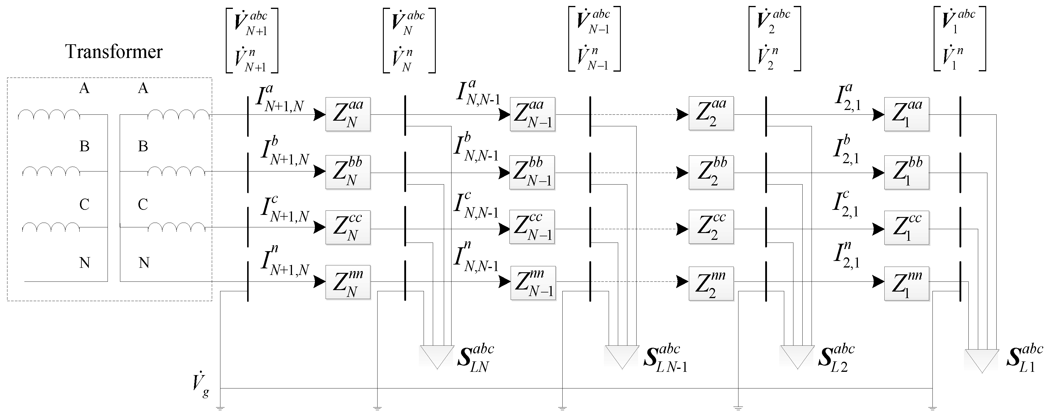
Under normal circumstances, the distribution system uses the radial operation structure. Thus, it is suitable to represent it with node branch incident matrix. Evidently, the number of nodes in the radial network is one more than that of the branches (the grounded branches are not considered). Suppose the element Aij in the node branch incident matrix A corresponds to the ith node, jth branch, which is directed from node m to n. Then Aij can be represented as:
A i j = { 1 1 0 i = m i = n i m , i n
Suppose the vector of currents injected into nodes in α (α = a, b, c) phase (with the power supply node excluded) is represented as I N α , and the vector of currents for the branch of α phase is represented as I L α . Then it has:
I N α = A I L α
where N is the total number of nodes of the distribution network excluding the power supply nodes. L is the total number of branches of the distribution network excluding the grounded branches. Thus, I L α can be calculated as:
I L α = A 1 I N α
(2)
Suppose the charging location of each EV is fixed. Only the optimization of the charging power is considered while the optimization of the charging location is not considered.
(3)
The fluctuation of the external power grid is not taken into account. The capacity of external power grid is assumed to be large enough and the substation bus is taken as the slack node in every optimization period.
(4)
It is assumed that the output power of the charger can be adjusted continuously.

2.2. Objective Functions and Constraints

The objective function of the first model is the power supply minimization of the distribution system shown as Equations (4) and (5)
J 1 = min t 1 t max J 0 ( t ) d t
J 0 ( t ) = n = 1 N α = 1 3 ( P P , n , α , t + P I , n , α , t + P Z , n , α , t ) + l = 1 L α = 1 3 R l , α ( I l , α , t r 2 + I l , α , t i 2 ) + k = 1 K α = 1 3 P EV k , α , t + m = 1 M P EV m , β , t
where t1 and tmax are the optimization start and end time, respectively. PP,n,α,t, PI,n,α,t, and PZ,n,α,t are the active power of the conventional household constant impedance, constant current and constant power load of node n phase α at time t, respectively. Rl,α and I l , α , t r + j I l , α , t i are the resistance and current of line l phase α at time t, respectively. PEVk,α,t and PEVm,β,t are the charging power of kth, mth EV with three-phase and single phase charging mode, located at phase α, β at time t, respectively. K and M are the total number of EVs with three-phase and single phase charging mode, respectively.
Due to the complexity of integral computation, in current research and practical control, the discretization technique is adopted. The total optimization time is divided into several periods. In each period, it is assumed that the conventional household load does not change and the charging power of each EV keeps constant. Thus, the objective function can be transformed as:
J 1 = min t = t 1 t max J 0 ( t ) Δ t
where ∆t is the interval of sampling and control.
The objective function of the second model is the minimization of energy costs that distribution system operator (DSO) purchases from the external power grid shown as (7):
J 2 = min t = t 1 t max ρ ( t ) J 0 ( t ) Δ t
where ρ ( t ) is the power price that the operator (DSO) purchases from outside at time t.
The objective function of the third model is the maximization of profit for DSO shown as:
J 3 = max t = t 1 t max ϕ ( t ) ( k = 1 K α = 1 3 P EV k , α , t + m = 1 M P EV m , β , t ) Δ t t = t 1 t max J 0 ( t ) Δ t j = 1 J β E j s h
where ϕ ( t ) is defined as 1.0 × 2 6 + 24 H ( t 18 ) t . λ is the penalty price that the DSO pays to the EVs holder, because the EVs are not fully charged. Suppose E j t end is the energy of jth EV when the optimization time is over and E j Cap is the capacity of the battery for the jth EV. E j s h = E j Cap E j t end is the energy cut down for the jth EV. The first term is the profits that the EVs are charged at early evening which is encouraged by the DSO. H(t) is the Heaviside step function. ϕ ( t ) is a very large value at early evening. The more energy EVs are charged at early evening, the more profits the DSO can make.
Constraint on the charging power of each EV with three-phase charging mode is:
0 P EV k , α , t P EV k , max
P EV k , a , t = P EV k , b , t = P EV k , c , t
Constraint on the charging power of each EV with single-phase charging mode is:
0 P EV m , β , t P EV m , max
where PEVk,max and PEVm,max are the maximal charging power of the kth and mth EV with three-phase and single phase charging mode, respectively.
Constraints on the power demand of each EV with three-phase and single phase charging mode for the first and second models are:
η α = 1 3 t = t k s t k e P EV k , α , t Δ t = E k cap E k ini
η t = t m s t m e P EV m , α , t Δ t = E m cap E m ini
where η is the charging efficiency. E k ini , E k cap , E m ini , and E m cap are the initial energy and the battery capacity of the kth, mth EV with three-phase and single-phase charging mode, respectively. tks, tke, tms, and tme are the charging start and end time for the kth, mth EV with three-phase and single-phase charging mode, respectively.
As for the third model constraints on power demand are:
η α = 1 3 t = t k s t k e P EV k , α , t Δ t E k cap E k ini
η t = t m s t m e P EV m , α , t Δ t E m cap E m ini
Constraint on nodal voltage of the distribution system is:
U min U n , α , t U max
where Un,α,t, Umin, and Umax are the voltage of node n, phase α at time t and its lower and upper limits, respectively.
Constraint on thermal loadings of each line is:
S l , α , t S l , max
where Sl,α,t and Sl,max are the power of the line l phase α at time t and its maximum, respectively.
Constraint on thermal loadings of each transformer is:
S T n , α , t S T max
where STn,α,t and STmax are the apparent power of the distribution transformer for phase α at time t and its maximum, respectively.
As for the first and second models, the constraints are Equations (9)–(18). As for the third model, the constraints are Equations (9)–(18).
In this paper, the technique of sensitivity analysis presented in [13] is introduced to linearize the constraints on nodal voltages and thermal loadings of transformers and lines.

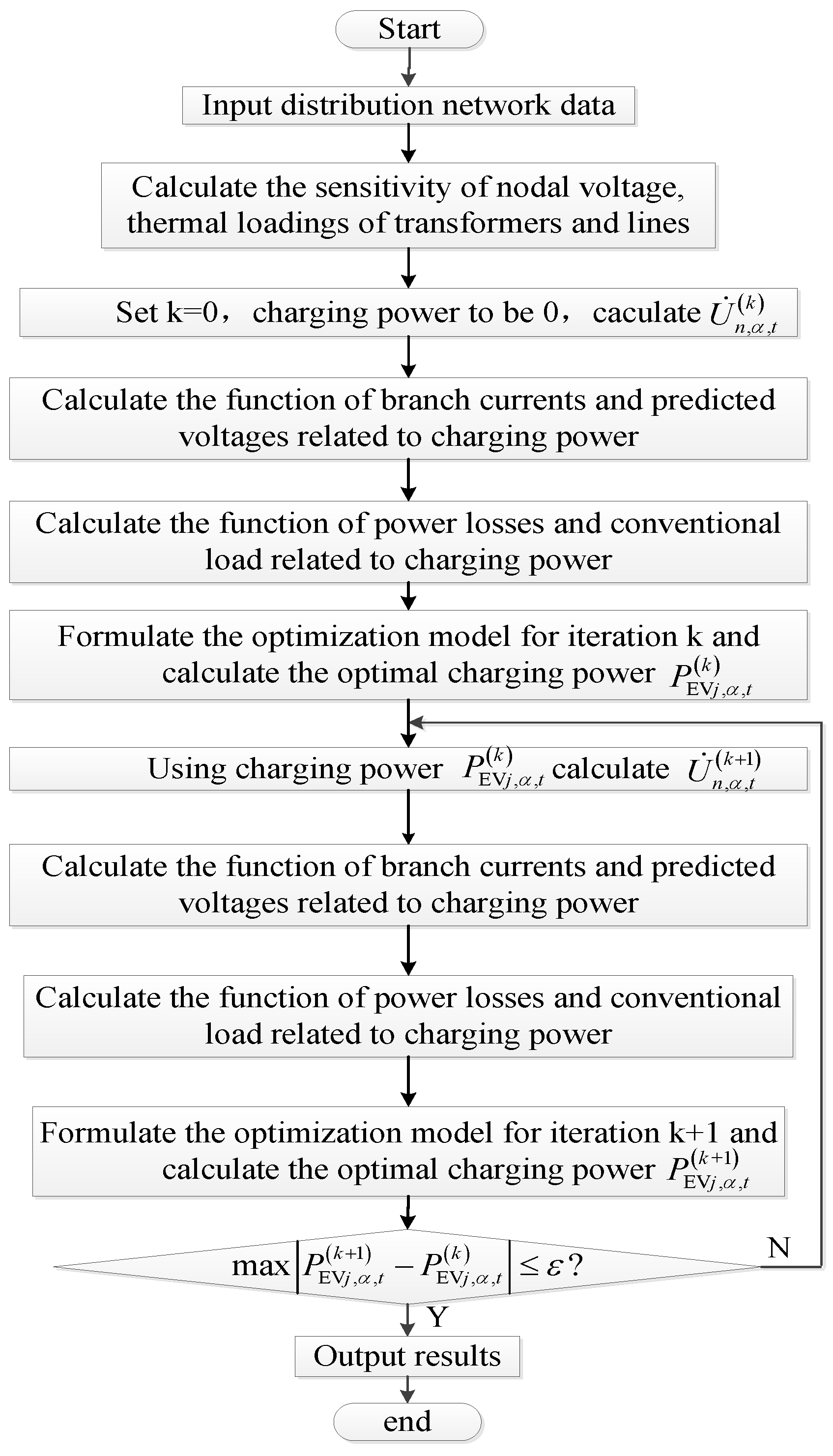
3. Extended Iterative Method

Nodal power balance equations are:
U ˙ n , α , t I ˙ n , α , t = S ˙ n , α , t
S ˙ n , α , t = ( P P , n , α , t + P I , n , α , t + P Z , n , α , t + P EV n , α , t ) + j ( Q P , n , α , t + Q I , n , α , t + Q Z , n , α , t )
P I , n , α , t = P I 0 , n , α , t ( U n , α , t U 0 , n , α , t )
P Z , n , α , t = P Z 0 , n , α , t ( U n , α , t U 0 , n , α , t ) 2
where QP,n,α,t, QI,n,α,t, and QZ,n,α,t are the reactive power of ZIP load on node n phase α at time t, respectively. PI0,n,α,t and PZ0,n,α,t are the active power of constant current and power conventional household load when the voltage on node n phase α at time t is U0,n,α,t, respectively. The current can be obtained from Equation (19), the formula for which is shown as:
I ˙ n , α , t = ( S ˙ n , α , t / U ˙ n , α , t ) n , α , t
It can be seen from Equations (3), (20)–(23) that the current of each line and its conjugate are the linear function of the charging power of EVs, assuming that the voltages are fixed to some known values. As the branch current magnitude square is equal to the current multiplied by its conjugate and power loss is a linear function of the current magnitude square, the power loss is the quadratic function of the charging power. However, when the conventional household load contains constant impedance and/or constant current load, the first term of J0 in Equation (5) is associated with nodal voltage. The conventional iterative methods in [11,12] cannot be applicable any more. To solve this problem, an extended iterative method is formulated as follows:
(P1)
Using the slack node as the root node, the depth first search (DFS) program is used to calculate the forward node sequence Pre and the parent node sequence Pred.
(P2)
At each iteration, using the complex voltage vector of root node, the branch impedance matrix and the branch current complex vector, node sequence Pre, Pred, the predicted voltage of each node per phase at time t related to charging power can successively be calculated as:
U ˙ pre ( i ) abc = U ˙ pred ( pre ( i ) ) abc Z pre ( i ) , pred ( pre ( i ) ) I ˙ pre ( i ) , pred ( pre ( i ) ) abc     i ,
where U ˙ pre ( i ) abc and U ˙ pred ( pre ( i ) ) abc are the three-phase predicted complex voltage vector of node Pre(i) and its parent node Pred(Pre(i)), respectively. Z pre ( i ) , pred ( pre ( i ) ) and I ˙ pre ( i ) , pred ( pre ( i ) ) abc are the impedance matrix and three-phase complex branch current vector between node Pre(i) and its parent node Pred(Pre(i)), respectively.
(P3)
The square of the predicted voltage magnitude of each node per phase at each time t is calculated with the complex voltage multiplied by its conjugate. Voltage magnitude can be obtained by root calculation.
(P4)
The active and reactive power of the conventional household load for each node per phase at each time t can be calculated by substituting the predicted voltage magnitudes into Equations (21) and (22).
By the above procedures P1~P4, the iterative method can be applicable once more. Clearly, the predicted voltage complex vector and its conjugate are linear functions of the charging power, such as Equation (24). Therefore, the square of the predicted voltage magnitude is the quadratic function of the charging power. If the conventional household load is only composed of constant power and/or constant impedance load, the active power of conventional household load is the quadratic function of the charging power. While if the conventional household load contains constant current load, the active power of the conventional household load is no longer the quadratic function of the charging power. But it is still a convex function of the charging power.
The flow chart of the proposed method is shown in Figure 2. The basic input information includes the topological structure of distribution system, parameters of distribution transformer and lines, load curves of each node per phase, charging locations, charging power limit, battery capacity, initial state of charge (SOC), charging start and end time of each EV, etc.
Suppose the charging power of each EV P EV j , α , t ( k ) is known, the voltage of each node per phase at time t, U ˙ n , α , t ( k + 1 ) can be calculated using power flow calculation. In this paper, the back/forward sweep method is used for power flow calculation. The node voltage U ˙ n , α , t ( k + 1 ) is then used as the known quantity, and a linear constrained convex quadratic programming or convex programming model is formulated at each iteration, and P EV j , α , t ( k + 1 ) is obtained.
The power flow is performed again with the charging power of each EV P EV j , α , t ( k + 1 ) used as the input information. The convergence criterion of the whole program is to maximize | P EV j , α , t ( k + 1 ) P EV j , α , t ( k ) | ε . When the difference of the infinity norm of a two adjacent optimal charging power vector is less than a pre-given small positive number, the procedure is terminated and the results are output.

4. Simulation Case Study

4.1. Simulation Case 1

A simple distribution system with two nodes is used to validate the precision of the proposed method. The single line diagram is shown in Figure 3. The base power and base voltage of each phase are 160/3 kVA and 10 / 3 kV, respectively. The voltage source is 1.05 p.u. The impedance matrix of the transmission lines is equal to:
Z Line = [ 00276 + 0.0124 i 0.0056 + 0.0060 i 0.0056 + 0.0060 i 0.0056 + 0.0060 i 0.0276 + 0.0124 i 0.0056 + 0.0060 i 0.0056 + 0.0060 i 0.0056 + 0.0060 i 0.0276 + 0.0124 i ]
The optimization period is 12:00~14:00. During the optimization period, there is a 40 kW and 80 kW conventional household load connected to bus 1 during the periods of 12:00~13:00 and 13:00~14:00, respectively. The power factor is 0.95. There are 10, 14 and 16 EVs connected to phase A, B, and C of bus 1, respectively. The power demand of each EV is 10 kWh. The upper limit of charging power of each EV is 10 kW. The upper and lower limit of the voltage are 1.10 p.u. and 0.90 p.u., respectively.
As for the objective function J1 and different load models, the optimization results of the proposed iterative method denoted as PM.0 and PM.1 are shown in Table 1, where f.0 and f.1 represent the optimization functions of MATLAB, fmincon, for charging periods of 12:00~13:00 and 13:00~14:00, respectively. Evidently, the optimization results of voltages and objective function are very close between PM.0 and f.0, as well as between PM.1 and f.1. However, the difference of optimal charging power between the proposed method and optimization functions is somewhat remarkable for the constant impedance load model.

4.2. Simulation Case 2

A distribution system with 14 nodes is used to validate the precision and the calculation speed of the proposed method. The single line diagram is shown in Figure 4. The parameters of the lines are shown in Table 2. The capacity of the transformer is 400 kVA. Both the positive and zero sequence impedance of the transformer are 0.06 + i0.0125 p.u. The base power and voltage of each phase are 160/3 kVA, 10 / 3 kV and 0.4 / 3 kV, respectively. Node 14 is the slack node and its voltage is 1.05 p.u. The optimization period is 12:00~14:00. During the periods of 12:00~13:00 and 13:00~14:00, the load connected to each node per phase is 3 kW and 1.5 kW, respectively. The power factor is 0.95. There is one EV connected to node 3~5, 8~10 phase A, node 7, 12 phase B, node 6, 11 phase C, respectively. The power demand of each EV connected to phase A, B, C are 10 kWh, 25 kWh, and 25 kWh, respectively. The upper limits of charging power of each EV connected to phase A, B, and C are 10 kW, 25 kW, and 25 kW, respectively. The upper and lower limits of the voltage are 1.10 p.u. and 0.90 p.u., respectively.
As for the objective function J1 and different load models, the optimization results are shown as Table A1, Table A2 and Table A3 in the Appendix A. The calculation results of voltages and objective functions are very close for PM.0 and f.0, as well as for PM.1 and f.1. However, the difference between optimal charging power between the proposed method and optimization functions is somewhat remarkable. The difference of the optimization results of the voltages, charging power, objective function between the proposed methods and the optimization function, fmincon, of MATLAB for constant impedance load is greater than that for the constant current load which is greater than that for the constant power load. This is because the charging power will cause the voltage drop, resulting in a decline in the power of conventional load. When the conventional household load is constant impedance load, the power of the conventional household load is proportional to the square of the voltage. The power decline is large. When the conventional household load is constant current load, the power of the conventional household load is proportional to the voltage. The power decline is small. When the conventional household load is constant power load, the power of the conventional household load is independent of voltage. The power declined is zero. Therefore, as for the proposed method, the sensitivity of the objective function to the charging power for constant impedance conventional household load is lower than that for constant current load which is lower than that for constant power load. As for constant impedance load, it can be seen that the difference caused by the sensitivity reduction is not much, as shown as Table A1, Table A2 and Table A3 in the Appendix A. The maximum difference of the charging power is less than 8%. The maximum difference of the voltage is less than 0.5%. The maximum difference of the objective function is less than 0.05%. However, the calculation time of the proposed method is much less than that of fmincon of MATLAB.

4.3. Simulation Case 3

4.3.1. Simulation Conditions

As shown in Figure 5, an actual distribution system with 141 nodes is introduced to test the capability of the proposed method. Length, impedance and rated current of lines are shown in Table 2. The transformer’s rated capacity is 400 kVA with both positive and zero sequence impedance are 0.06 + i0.0125 p.u. As shown by the arrows in Figure 5, there are total 165 households in the distribution system. The lumped load is connected to phase A. It indicates 31 single phase household loads of another area. While the rest 134 household loads indicate three-phase symmetrical ones. As shown by the small black circles in Figure 5, there are 67 EVs distributed in the distribution system. Taking one EV per household for example, the permeability of EV is 50%. Charging locations of each EV is the same as the household load. As the load curve of each household is not available, typical summer load curves between 18:00~7:00 as shown in Figure 6 is assigned to each household. Different load curves may result in different optimal charging power curves for each EV. However, the capability of the algorithm is independent of load curves.
Other simulation conditions are set as follows:
(1)
All EV owners are willing to participate in coordinated charging and charging power of each EV is fully controllable. Optimization period of time is between 18:00~7:00.
(2)
Maximal charging power of each EV is 4 kW. The battery capacity of each EV is 20 kWh. Charging efficiency is 0.98. As for J1, J2, J3, initial SOC of each EV is set to be 0.25, 0.5, and 0.5, respectively.
(3)
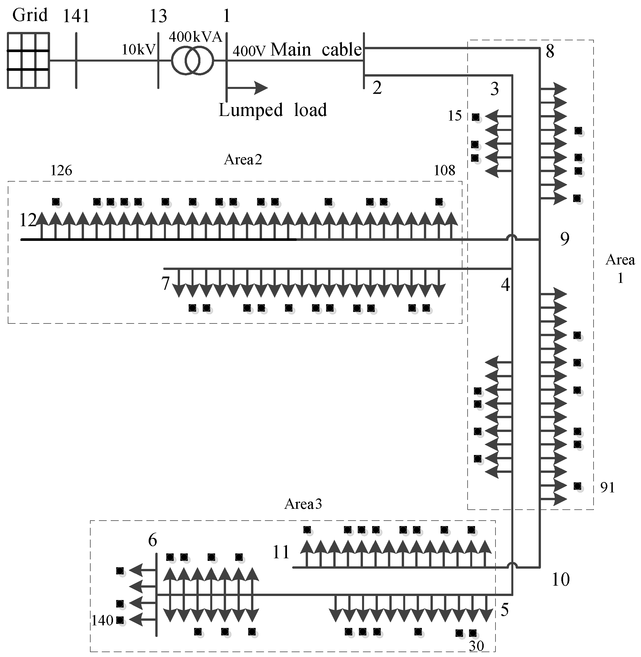
Each EV adopts single phase charging mode. EVs located at area 1, 2 and 3 are connected to phase A, B, and C, respectively.
(4)
The optimization time interval is 1 h.
(5)
The upper and lower voltage limit are 1.1 p.u. and 0.9 p.u., respectively.
(6)
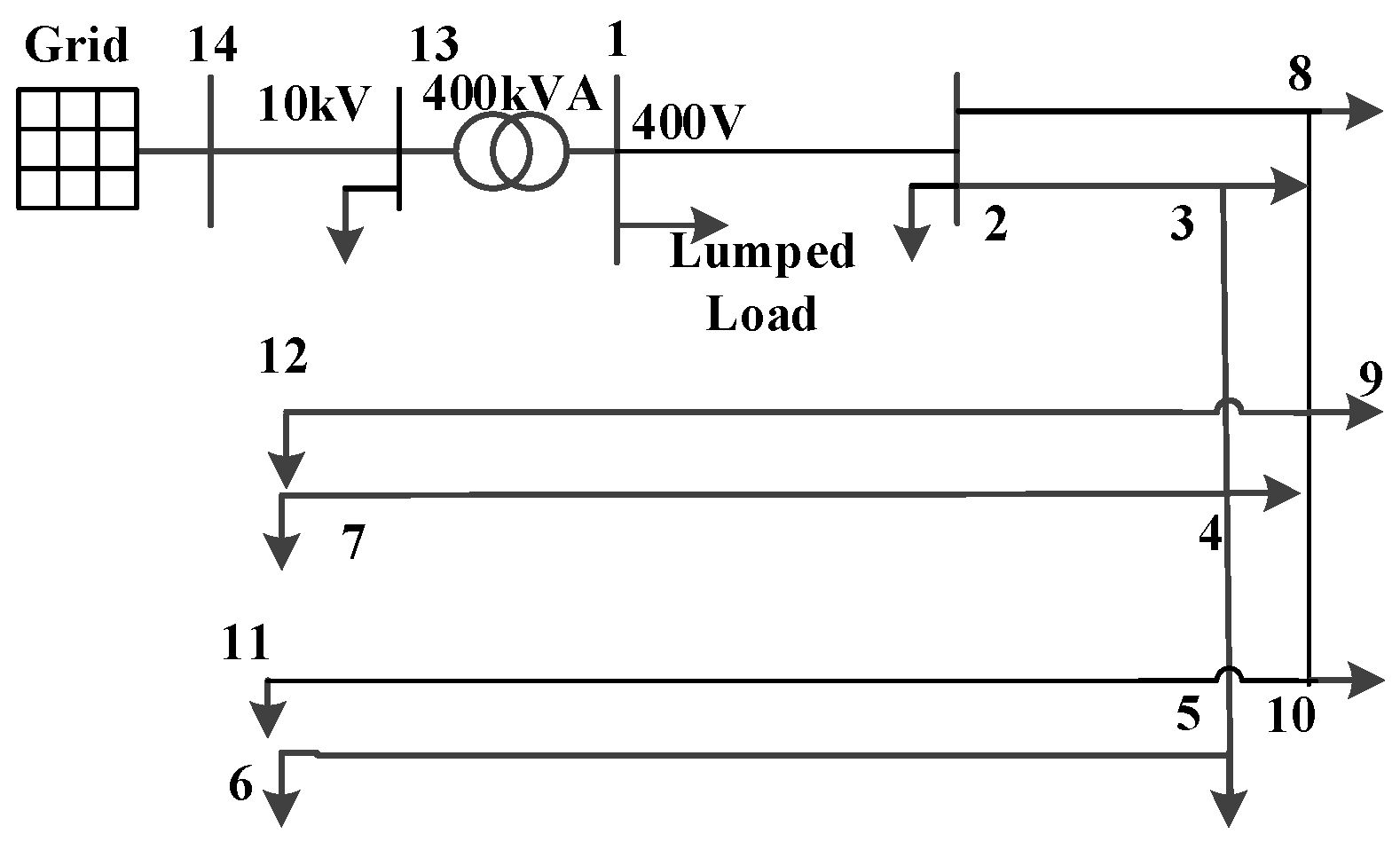
Node 141 is taken as the slack node, and its voltage is kept constant as 1.05 p.u. The rest of the nodes are taken as PQ nodes.
(7)
As for objective J2 and J3, during the optimization periods, the charging price is 0.77, 0.75, 0.70, 0.70, 0.66, 0.60, 0.48, 0.36, 0.34, 0.30, 0.28, 0.27, 0.27, 0.29 Y/kWh, and β is set to be 100.
(8)
The model of the conventional household load is assumed to be constant impedance load.
(9)
The single phase based power and voltage of the system is 160/3 kVA, 10 / 3 kV, and 0.4 / 3 kV, respectively.

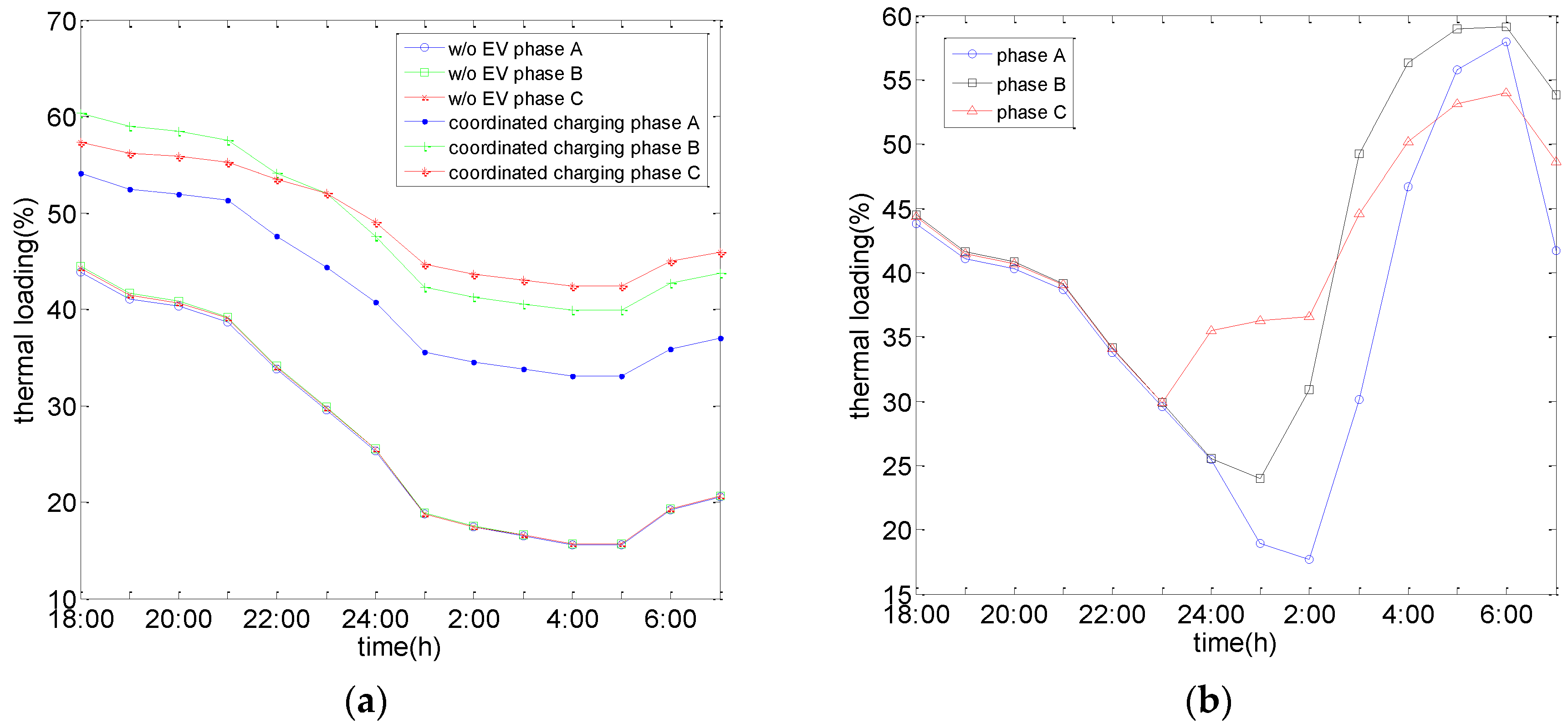
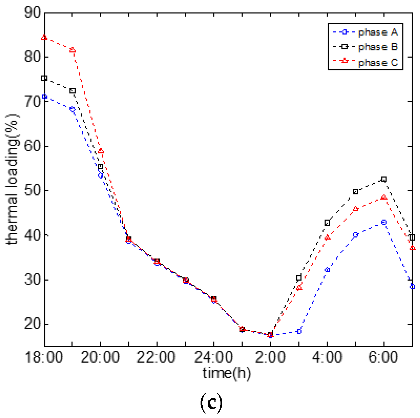
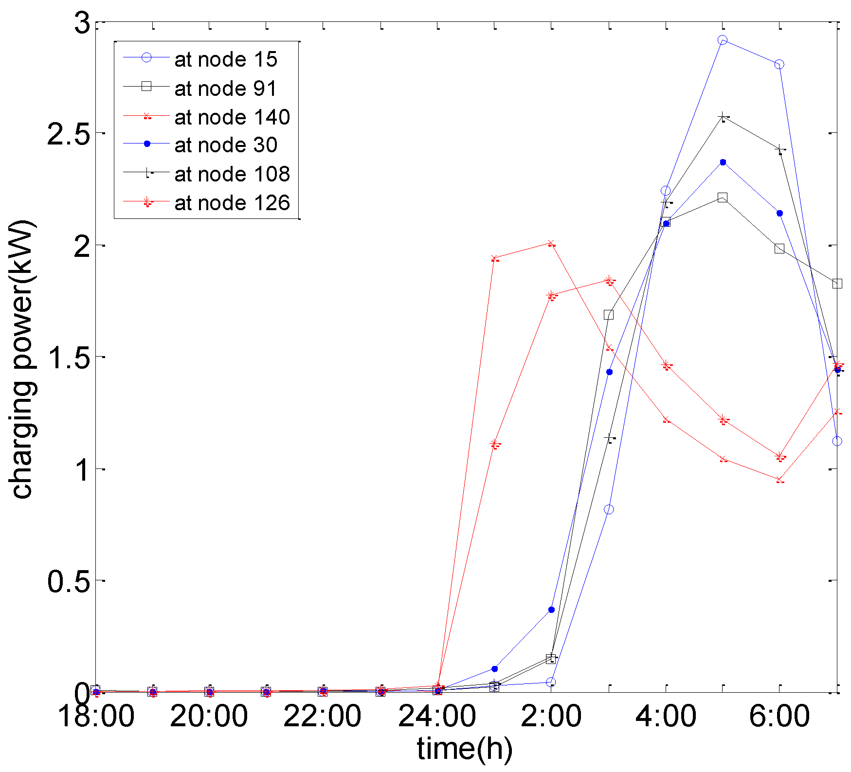
4.3.2. Simulation Results

Typically, the program converges within five iterations. Charging power of some EVs located at typical nodes for different objective functions are shown in Figure 7, Figure 8 and Figure 9. It can be seen that the charging power of EVs located at different nodes vary from each other greatly. As for the objective function J1, in the evening peak time, the charging power of EVs is large to reduce the conventional household load power by lowering the voltage. As for EV located at node 15, the charging power is maximal in the evening peak time while it is minimal at late night trough time. This is because node 15 is near to the start of the distribution system, the network losses of additional current caused by this charging load is low. Charging with a higher power at the peak time can lower the voltage. Thus, the power of the conventional household load can be reduced. As for EVs located at node 91, 140, 30, 108, 126, the charging power at peak time is lower than that at trough time. This is because these nodes are far from the start of the distribution system. Increasing the charging power at trough time can effectively reduce the network losses of the additional current caused by the charging power.
Charging power is also closely associated with the power price. As for the objective function J2, when the power price is low, the charging power is high. Conversely, when the power price is high, the charging power is low (even zero). As for objective function J3, the charging power of the EVs with priority such as those connected to node 15, 140, and 126 is very high during peak time in order to get fully charged as soon as possible for use in the early evening. As for the EVs without priority such as those connected to node 91, 30, 108, the charging power is high when the power price is low. Conversely, when the power price is high, the charging power of those EVs is low (even zero).
Total charging power of EVs, total conventional household load of household, total power losses and total power supply of the distribution system for different objective functions are shown in Figure 10. As for the objective function J1, the total charging power is somewhat uniform. At the peak time, it is slightly higher than that at the trough time. The total power supply is similar to that of the total conventional load. As for objective J2, the total charging load is concentrated on the time when the power price is low. In the peak power price time, the total charging power is very small, even zero. As for objective J3, the total charging load is concentrated in the early evening and the low power price time.
Thermal loadings of transformer for different objective functions are shown in Figure 11. Clearly, it increases significantly during the periods when the charging power is high. But all of them are less than 80%.
Thermal loadings of the main cable for different objective functions are shown in Figure 12. Clearly, it increases significantly during the periods when the charging power is high, but all of them are less than 85%. It is evident that neither the currents of transformer nor those of main cable are the binding constraints on this network. Clearly, the network equipment is more than well suited to accommodate the additional load required by the high penetration of EVs, assuming the proposed coordinated charging scheme is introduced.
The three-phase voltage profiles of node 6, which is located at the terminal of the distribution system are shown as Figure 13. As the lumped load is connected to phase A, the voltage of phase A for node 6 is slightly lower than that of phase B and C when charging power is low. Clearly, the high charging load results in a significant drop in voltage. If the voltage constraint is not applied, the voltage of phase C is much lower than that of the lower bound. However, if the voltage constraint is applied, the voltage of all the three phase is above that of the lower bound. Thus, the voltage is really a binding constraint when there are a large amount of EVs connected to the distribution network.

4.3.3. Comparison with the Selected Method

The optimization results of the proposed method compared with the method in [15] are shown as Table 3. Clearly, the calculation efficiency of the proposed method is much higher than the method described in [15]. This is because at each iteration, optimization variables only consist of the charging power of EVs, which greatly reduce the number of optimization variables. Whereas, in [15] nodal voltages are included in the optimization variables. Although linearization techniques are applied and mixed integer linear programming is formulated, because the number of optimization variables is large, the calculation time increases greatly.
From the simulation results, it can be seen that the proposed method has a rapid convergence rate in the optimization of large-scale coordinated charging of EVs, and can greatly improve the economic benefits and guarantee the safe operation of distribution system.

5. Conclusions

In this paper, three models for smart charging of EVs were formulated to minimize the total power supply, power costs and maximize the operation profits. The iterative method was extended to solve the developed models. The extended algorithm was accommodated to a mix of ZIP load of the conventional household with the three-phase imbalance of distribution network, constraints on nodal voltages and thermal loadings of transformers and lines taken into account. When the conventional household load was composed of constant impedance and/or constant power loads, a linearly constrained convex quadratic programming model could be formulated at each iteration. When the conventional household load consists of the constant current load, a linear constrained convex programming model could be formulated instead.
The simulation results indicate that:
(1)
Compared with the optimization results in [15], the developed method had much higher calculation efficiency.
(2)
This developed method could avoid the risk of the node voltage exceeding the lower limit, and provided reliable and economic operation of the distribution system when massive numbers of EVs penetrate into the grid.

Acknowledgments

This work was supported by the National Natural Science Foundations of China (under Grant 51577046, 5160070415, and 51107090), the National Defense Advanced Research Project (under Grant C1120110004 and 9140A27020211DZ5102), the Key Grant Project of Chinese Ministry of Education (under Grant 313018), the Anhui Provincial Science and Technology Foundation of China (under Grant 1301022036), the National Research Foundation for the Doctoral Program of Higher Education of China (under Grant JZ2015HGBZ0095), and the State Key Program of National Natural Science of China (under Grant 51637004).

Author Contributions

Jian Zhang and Yigang He conceived and designed the methodology; Jian Zhang and Hualiang Fang performed the case studies and analysis; Jian Zhang and Mingjian Cui wrote the paper.

Conflicts of Interest

The authors declare no conflict of interest.

Appendix A

Table A1. Constant impedance load model.
Different MethodPM.0PM.1f.0f.1
1UA/p.u.0.99521.00970.99431.0105
UB/p.u.0.99831.01290.99761.0136
UC/p.u.0.99741.01190.99661.0126
2UA/p.u.0.95450.97810.95300.9796
UB/p.u.0.96230.98600.96110.9873
UC/p.u.0.96070.98420.95940.9856
3UA/p.u.0.94980.97440.94820.9760
UB/p.u.0.95820.98290.95690.9842
UC/p.u.0.95650.98090.95510.9824
4UA/p.u.0.94070.96680.93860.9689
UB/p.u.0.94660.97350.94500.9750
UC/p.u.0.94510.97160.94340.9732
5UA/p.u.0.93590.96300.93360.9654
UB/p.u.0.94480.97350.94340.9749
UC/p.u.0.93270.96000.93070.9619
6UA/p.u.0.93640.96550.93420.9677
UB/p.u.0.94340.97400.94210.9754
UC/p.u.0.90830.93530.90550.9381
7UA/p.u.0.93950.96710.93750.9691
UB/p.u.0.92800.95470.92570.9569
UC/p.u.0.94530.97340.94380.9749
8UA/p.u.0.94920.97390.94760.9755
UB/p.u.0.95770.98250.95630.9837
UC/p.u.0.95610.98060.95460.9820
9UA/p.u.0.94280.96850.94080.9705
UB/p.u.0.94930.97580.94790.9771
UC/p.u.0.94810.97410.94640.9757
10UA/p.u.0.93770.96450.93540.9667
UB/p.u.0.94740.97580.94610.9771
UC/p.u.0.93490.96170.93290.9638
11UA/p.u.0.93800.96570.93590.9679
UB/p.u.0.94660.97580.94530.9770
UC/p.u.0.92440.95100.92190.9535
12UA/p.u.0.94080.96920.93890.9710
UB/p.u.0.91500.94150.91270.9438
UC/p.u.0.94860.97740.94720.9789
13UA/p.u.1.00691.01751.00621.0182
UB/p.u.1.00961.02011.00901.0207
UC/p.u.1.00871.01921.00801.0198
PCH3A/p.u.0.10230.08520.09520.0923
PCH4A/p.u.0.08300.10430.09150.0960
PCH5A/p.u.0.08320.10430.09100.0965
PCH8A/p.u.0.10000.08750.09450.0928
PCH9A/p.u.0.08340.10410.09130.0962
PCH10A/p.u.0.08310.10440.09130.0962
PCH7B/p.u.0.22080.24800.23000.2387
PCH12B/p.u.0.22230.24640.22920.2395
PCH6C/p.u.0.22120.24750.22900.2398
PCH11C/p.u.0.22080.24800.23020.2385
J1/p.u.6.62786.6275
Calculation time/s0.736167
Table A2. Constant current load model.
Different MethodPM.0PM.1f.0f.1
1UA/p.u.0.99631.00640.99571.0070
UB/p.u.0.99551.01050.99801.0110
UC/p.u.0.99781.00920.99721.0097
2UA/p.u.0.95700.97170.95590.9727
UB/p.u.0.96270.98190.96180.9829
UC/p.u.0.96130.97950.96030.9805
3UA/p.u.0.95250.96750.95140.9686
UB/p.u.0.95870.97850.95770.9795
UC/p.u.0.95710.97600.95600.9771
4UA/p.u.0.94340.95940.94200.9608
UB/p.u.0.94760.96820.94640.9694
UC/p.u.0.94570.96610.94440.9673
5UA/p.u.0.93870.95530.93720.9569
UB/p.u.0.94550.96840.94440.9695
UC/p.u.0.93380.95350.93230.9550
6UA/p.u.0.93860.95820.93720.9596
UB/p.u.0.94370.96910.94260.9701
UC/p.u.0.91080.92680.90880.9289
7UA/p.u.0.94190.95990.94060.9612
UB/p.u.0.93070.94730.92900.9490
UC/p.u.0.94540.96830.94430.9694
8UA/p.u.0.95190.96700.95080.9682
UB/p.u.0.95810.97820.95710.9792
UC/p.u.0.95680.97550.95570.9767
9UA/p.u.0.94550.96130.94420.9626
UB/p.u.0.94980.97100.94870.9721
UC/p.u.0.94910.96840.94780.9697
10UA/p.u.0.94040.95700.93890.9584
UB/p.u.0.94750.97120.94650.9723
UC/p.u.0.93680.95480.93530.9563
11UA/p.u.0.94040.95850.93900.9598
UB/p.u.0.94650.97130.94550.9723
UC/p.u.0.92720.94290.92540.9448
12UA/p.u.0.94300.96210.94180.9634
UB/p.u.0.91760.93390.91570.9357
UC/p.u.0.94890.97230.94780.9734
13UA/p.u.1.00801.01481.00761.0152
UB/p.u.1.01001.01821.00951.0187
UC/p.u.1.00921.01691.00881.0174
PCH3A/p.u.0.08560.10190.08270.1048
PCH4A/p.u.0.07420.11330.07810.1094
PCH5A/p.u.0.07380.11370.078710.1088
PCH8A/p.u.0.08510.10240.08330.1042
PCH9A/p.u.0.07440.11310.07920.1083
PCH10A/p.u.0.07360.113890.07780.1097
PCH7B/p.u.0.19420.27450.20070.2681
PCH12B/p.u.0.20390.26480.20910.2596
PCH6C/p.u.0.20270.26600.20840.2604
PCH11C/p.u.0.19510.27370.20160.2671
J1/p.u.6.76956.7693
Calculation time/s0.812185
Table A3. Constant power load model.
Different MethodPM.0PM.1f.0f.1
1UA/p.u.0.99761.00250.99751.0026
UB/p.u.0.99891.00770.99881.0078
UC/p.u.0.99831.00600.99821.0061
2UA/p.u.0.95990.96430.95990.9643
UB/p.u.0.96330.97710.96300.9774
UC/p.u.0.96210.97400.96190.9742
3UA/p.u.0.95560.95970.95560.9597
UB/p.u.0.95940.97340.95910.9737
UC/p.u.0.95790.97030.95760.9705
4UA/p.u.0.94670.95090.94670.9509
UB/p.u.0.94870.96210.94840.9624
UC/p.u.0.94650.95960.94620.9600
5UA/p.u.0.94200.94650.94200.9465
UB/p.u.0.94630.96240.94600.9627
UC/p.u.0.93520.94600.93480.9464
6UA/p.u.0.94130.94970.94140.9496
UB/p.u.0.94420.96320.94390.9635
UC/p.u.0.91370.91690.91320.9175
7UA/p.u.0.94480.95150.94490.9515
UB/p.u.0.93370.93890.93340.9393
UC/p.u.0.94570.96220.94540.9625
8UA/p.u.0.95510.95920.95500.9592
UB/p.u.0.95860.97310.95830.9734
UC/p.u.0.95770.96970.95750.9699
9UA/p.u.0.94870.95300.94870.9530
UB/p.u.0.95050.96550.95020.9658
UC/p.u.0.95030.96180.95000.9621
10UA/p.u.0.94360.94840.94360.9484
UB/p.u.0.94780.96590.94750.9662
UC/p.u.0.93900.94670.93870.9471
11UA/p.u.0.94320.95010.94330.9501
UB/p.u.0.94670.96600.94630.9664
UC/p.u.0.93040.93360.93000.9340
12UA/p.u.0.94570.95400.94570.9540
UB/p.u.0.92040.92520.91990.9258
UC/p.u.0.94940.96620.94920.9664
13UA/p.u.1.00941.01161.00931.0117
UB/p.u.1.01051.01601.01031.0161
UC/p.u.1.00991.01431.00981.0144
PCH3A/p.u0.06710.12040.06820.1193
PCH4A/p.u0.06500.12250.06320.1243
PCH5A/p.u0.06420.12330.06510.1224
PCH8A/p.u0.06860.11890.07010.1174
PCH9A/p.u0.06530.12220.06580.1217
PCH10A/p.u0.06390.12360.06280.1247
PCH7B/p.u0.16580.30290.16670.3021
PCH12B/p.u0.18410.28460.18580.2829
PCH6C/p.u0.18290.28590.18450.2843
PCH11C/p.u0.16760.30110.16870.3000
J1/p.u.6.93226.9322
Calculation time/s0.645131

References

  1. Tao, S.; Xiao, X.; Peng, C. Active Smart Distribution Network; China Electric Power Press: Beijing, China, 2012. [Google Scholar]
  2. Richardson, P.; Flynn, D.; Keane, A. Impact assessment of varying penetrations of electric vehicles on low voltage distribution systems. In Proceedings of the IEEE Power and Energy Society General Meeting, Minneapolis, MN, USA, 25–29 July 2010.
  3. Edwin, H.; Johan, D.; Ronnie, B. Robust planning methodology for integration of stochastic generators in distribution grids. IET Renew. Power Gener. 2007, 1, 25–32. [Google Scholar]
  4. Singh, M.; Kumar, P.; Kar, I. Implementation of vehicle to grid infrastructure using fuzzy logic controller. IEEE Trans. Smart Grid 2012, 3, 565–577. [Google Scholar] [CrossRef]
  5. Singh, M.; Thirugnanam, K.; Kumar, P.; Kar, I. Real-time coordination of electric vehicles to support the grid at the distribution substation level. IEEE Syst. J. 2015, 9, 1000–1010. [Google Scholar] [CrossRef]
  6. Beaude, O.; He, Y.; Hennebel, M. Introducing decentralized EV charging coordination for the voltage regulation. In Proceedings of the 2013 4th IEEE PES Innovative Smart Grid Technologies Europe (ISGT Europe), Copenhagen, Denmark, 6–9 October 2013.
  7. Deilami, S.; Masoum, A.S.; Moses, P.S.; Masoum, M.A.S. Real time coordination of plug in electric vehicle charging in smart grids to minimize power losses and improve voltage profile. IEEE Trans. Smart Grid 2011, 3, 456–467. [Google Scholar] [CrossRef]
  8. Masoum, A.S.; Deilami, S.; Moses, P.S.; Abu-Siada, A. Smart load management of plug-in electric vehicles in distribution and residential networks with charging stations for peak shaving and loss minimization considering voltage regulation. IET Gener. Transm. Distrib. 2011, 5, 877–888. [Google Scholar] [CrossRef]
  9. Li, H.; Bai, X.; Tan, W.; Dong, W.; Li, N. Application of vehicle to grid to the distribution grid. Proc. CSEE 2012, 32, 22–27. [Google Scholar]
  10. Sun, J.; Wan, Y.; Zheng, P.; Lin, X. Coordinated charging and discharging strategy for electric vehicles based on demand side management. Trans. China Electro-Tech. Soc. 2014, 29, 64–69. [Google Scholar]
  11. Zhan, K.; Song, Y.; Hu, Z.; Xu, Z.; Jia, L. Coordination of electric vehicle charging to minimize active power losses. Proc. CSEE 2012, 32, 11–18. [Google Scholar]
  12. Clement-Nyns, K.; Haesen, E.; Driesen, J. The impact of charging plug in hybrid electric vehicles on a residential distribution grid. IEEE Trans. Power Syst. 2010, 25, 371–380. [Google Scholar] [CrossRef] [Green Version]
  13. Richardson, P.; Flynn, D.; Keane, A. Optimal charging of electric vehicles in low voltage distribution systems. IEEE Trans. Power Syst. 2012, 27, 268–279. [Google Scholar] [CrossRef]
  14. Richardson, P.; Flynn, D.; Keane, A. Local versus centralized charging strategies for electric vehicles in low voltage distribution systems. IEEE Trans. Smart Grid 2012, 3, 1020–1028. [Google Scholar] [CrossRef]
  15. Franco, J.F.; Rider, M.J.; Romero, R. A mixed integer linear programming model for the electric vehicle charging coordination problem in unbalanced electrical distribution systems. IEEE Trans. Smart Grid 2015, 6, 2200–2210. [Google Scholar] [CrossRef]
  16. He, Y.; Venkatesh, B.; Guan, L. Optimal scheduling for charging and discharging of electric vehicles. IEEE Trans. Smart Grid 2012, 3, 1095–1105. [Google Scholar] [CrossRef]
  17. Hu, J.; You, S.; Lind, M.; Ostergaard, J. Coordinated charging of electric vehicles for congestion prevention in the distribution grid. IEEE Trans. Smart Grid 2014, 5, 703–711. [Google Scholar] [CrossRef] [Green Version]
  18. Weckx, S.; Driesen, J. Load balancing with EV chargers and PV inverters in unbalanced distribution grids. IEEE Trans. Sustain. Energy 2015, 6, 635–643. [Google Scholar] [CrossRef]
  19. Sortomme, E.; Hindi, M.M.; James, S.D.; Pherson, M.; Venkata, S.S. Coordinated charging of plug in hybrid electric vehicles to minimize distribution system losses. IEEE Trans. Smart Grid 2011, 2, 198–205. [Google Scholar] [CrossRef]
Figure 1. Schematic diagram of a simple distribution system.
Energies 09 00985 g001
Figure 2. Flow chart of the proposed algorithm for smart charging of EVs.
Energies 09 00985 g002
Figure 3. Single line diagram of a 2-node distribution system.
Energies 09 00985 g003
Figure 4. Single line diagram of a 14-node distribution system.
Energies 09 00985 g004
Figure 5. The single line diagram of an actual distribution system with 141 nodes.
Energies 09 00985 g005
Figure 6. Load curves of household.
Energies 09 00985 g006
Figure 7. Optimal charging power of EVs at typical nodes for the objective function J1.
Energies 09 00985 g007
Figure 8. Optimal charging power of EVs at typical nodes for J2.
Energies 09 00985 g008
Figure 9. Optimal charging power of EVs at typical nodes for J3.
Energies 09 00985 g009
Figure 10. Relationship between charging load and conventional household load for J1, J2, and J3. (a) Relationship between charging load and conventional household load for J1; (b) Relationship between charging load and conventional household load for J2; (c) Relationship between charging load and conventional household load for J3.
Energies 09 00985 g010
Figure 11. Thermal loadings of transformer for J1, J2, and J3. (a) Thermal loadings of transformer for J1; (b) Thermal loadings of transformer for J2; (c) Thermal loadings of transformer for J3.
Energies 09 00985 g011
Figure 12. Thermal loadings of main cable for J1, J2, and J3. (a) Thermal loadings of main cable for J1; (b) Thermal loadings of main cable for J2; (c) Thermal loadings of main cable for J3.
Energies 09 00985 g012aEnergies 09 00985 g012b
Figure 13. Voltage of node 6 under different scenarios for J1, J2, and J3. (a) Voltage of node 6 under different scenarios for J1; (b) Voltage of node 6 under different scenarios for J2; (c) Voltage of node 6 under different scenarios for J3.
Energies 09 00985 g013
Table 1. Optimization results for different load models.
Constant Current Load Model
Different MethodPM.0PM.1f.0f.1
U A /p.u.0.96870.98450.96960.9836
U B /p.u.0.95440.96990.95520.9691
U C /p.u.0.95500.97050.95580.9697
P CHA /p.u.0.77341.10160.74751.1275
P CHB /p.u.1.14421.48081.12031.5047
P CHC /p.u.1.32811.67191.30681.6932
J 1 /p.u.15.226415.2263
Constant impedance load model
Different methodPM.0PM.1f.0f.1
U A /p.u.0.96340.99210.96520.9902
U B /p.u.0.95000.97790.95160.9761
U C /p.u.0.95020.97820.95190.9765
P CHA /p.u.0.98270.89230.92770.9473
P CHB /p.u.1.34601.27831.29541.3296
P CHC /p.u.1.52621.47381.47931.5207
J 1 /p.u.14.970314.9696
Constant power load model
Different methodPM.0PM.1f.0f.1
U A /p.u.0.97470.97620.97480.9761
U B /p.u.0.95950.96100.95960.9609
U C /p.u.0.96040.96190.96050.9618
P CHA /p.u.0.55931.31570.55691.3181
P CHB /p.u.0.93371.69130.93121.6938
P CHC /p.u.1.12101.87901.11841.8816
J 1 /p.u.15.502015.5020
Table 2. The parameters of distribution system.
LineL(m) R 1 ( Ω ) X 1 ( Ω ) R 0 ( Ω ) X 0 ( Ω ) I N ( A )
MV100020.8410121000
1–21900.00320.0140.0950.041510
2–327.50.0080.0020.0240.006368
3–4850.0240.0060.0730.018368
4–597.50.0280.0070.0840.021368
5–61540.0620.0110.1850.033300
4–71190.0480.0090.1430.026300
2–832.50.0090.0020.0280.007368
8–9590.0170.0040.0510.013368
9–101060.0300.0080.0910.023368
10–11950.0270.0070.0820.021368
9–122170.0870.0160.2610.047368
Table 3. Optimization results compared with [15].
Different MethodsDifferent ModelsObjective FunctionMinimal VoltageCalculation Time
The proposed method J 1 /p.u.49.91630.900219 s
J 2 /Yuan1039.60.900021 s
J 3 /Yuan31,331.70.900022 s
The method in [15] J 1 /p.u.49.92660.9005723 s
J 2 /Yuan1040.90.9000746 s
J 3 /Yuan31,331.90.9000757 s

