Global Maximum Power Point Tracking (MPPT) of a Photovoltaic Module Array Constructed through Improved Teaching-Learning-Based Optimization

Abstract

The present study proposes a maximum power point tracking (MPPT) method in which improved teaching-learning-based optimization (I-TLBO) is applied to perform global MPPT of photovoltaic (PV) module arrays under dissimilar shading situations to ensure the maximum power output of the module arrays. The proposed I-TLBO enables the automatic adjustment of teaching factors according to the self-learning ability of students. Incorporating smart-tracking and self-study strategies can effectively improve the tracking response speed and steady-state tracking performance. To evaluate the feasibility of the proposed I-TLBO, a HIP-2717 PV module array from Sanyo Electric was employed to compose various arrays with different serial and parallel configurations. The arrays were operated under different shading conditions to test the MPPT with double, triple, or quadruple peaks of power-voltage characteristic curves. Boost converters were employed with TMS320F2808 digital signal processors to test the proposed MPPT method. Empirical results confirm that the proposed method exhibits more favorable dynamic and static-state response tracking performance compared with that of conventional TLBO.

1. Introduction

A photovoltaic (PV) power generation system is composed of a PV module array, a power conditioner, and a power transmission and distribution system. Because the output power of a PV module array changes substantially under the effect of insolation and environmental temperature changes [1], power conditioners not only function as inverters, but also require a maximum power point (MPP) tracker to control the PV module array. Consequently, power loss in the PV module array can be reduced while maintaining MPP output under different environmental conditions.

Different sets of power–voltage (P–V) characteristic curves can be generated for different insolation and environmental temperature. To ensure the maximum power output, the duty cycles of a power converter are commonly adopted. Concerning conventional maximum power point tracking (MPPT) techniques, they include the most frequently adopted perturb and observe (P&O) [2,3,4] and incremental conductance (INC) [5,6] methods. Although the P&O method is simple and involves only a few parameters, a drawback of this method is that users must choose between tracking speed and number of oscillations, in which favorable performance of one comes at the expense of the other. By contrast, the INC method improves tracking speed but features unfavorable tracking stability because precision sensors are required to measure the conductance. Moreover, when PV array modules are faulty or subjected to partial shading, the corresponding P–V characteristic curves exhibit multiple peaks [7]. Thus, applying these two conventional MPPT methods generates local MPPs rather than global MPPs. Shaded modules in a PV array are known to incur mismatching problems. In this context, the global MPP cannot be successfully tracked using a typical Field MPPT, that is to say, deteriorated power generation efficiency, due to the multiple peaks on a P–V characteristic curve. A distributed maximum power point tracker (DMPPT) was proposed as a way to resolve this mismatching problem and hence to elevate the overall power generation efficiency [8,9]. However, a clear disadvantage of a DMPP tracker is a rise in the cost and more room occupied. For this sake, to develop a low cost, but high performance, global MPP tracker to deal with the multi-peak problems on a P–V characteristic curve for the optimal performance of a PV array is an important research effort.

In recent years, numerous scholars have investigated MPPT methods for PV module arrays exhibiting multiple peaks under partial shading. Commonly adopted intelligent algorithms include the differential evolution (DE) [10], the ant colony optimization (ACO) [11], and the artificial bee colony (ABC) algorithms [12]. The DE algorithm, similar to a genetic algorithm [13,14], performs real number coding on selected groups to search for a global optimal solution through the differential calculation of variance and one-to-one competitive survival strategies. However, as demonstrated in [15], only simulation results were presented. In addition, individual mutation strategies were based on a total of five equations proposed by Storn [16], which not only increases tracking-time calculations, but also requires a more accurate comparison between population codes during crossover coding with microcontrollers. The ACO algorithm is a probabilistic path optimization algorithm based on the foraging behaviors of ants. The pheromones that ants lay down when they find food are used as a food-source indicator, with which other ants can determine the optimal food-finding path; this conserves time otherwise spent on random searching. In [17], pheromone update equations were expressed as exponential functions that yielded random values for transitioning between controlling the pheromone density and path length. Although this approach eliminates the possibility of identifying local optimal solutions, calculating the path length by using exponential functions requires considerably longer tracking time. The ABC algorithm transmits information regarding the quality and position of a food source through the “dance” performed by employed bees, which are responsible for finding larger food sources to increase profitability during the colony food-finding optimization process [18]. However, the employed bee phase relies on random values, resulting in an unstable searching capacity. In addition, in the scout phase, the number of bees selected affects the tracking speed and steady-state performance. As mentioned in [18], obtaining the statistical results of ABC and particle swarm optimization (PSO) algorithms requires 5–6 s, indicating that the tracking response speed can be improved. Moreover, scholars have proposed incorporating intelligent algorithms with conventional MPPT algorithms [19,20,21,22], such as incorporating PSO or genetic algorithms with P&O. Although the incorporated methods can successfully identify global optimal solutions, the dynamic response speed is too slow.

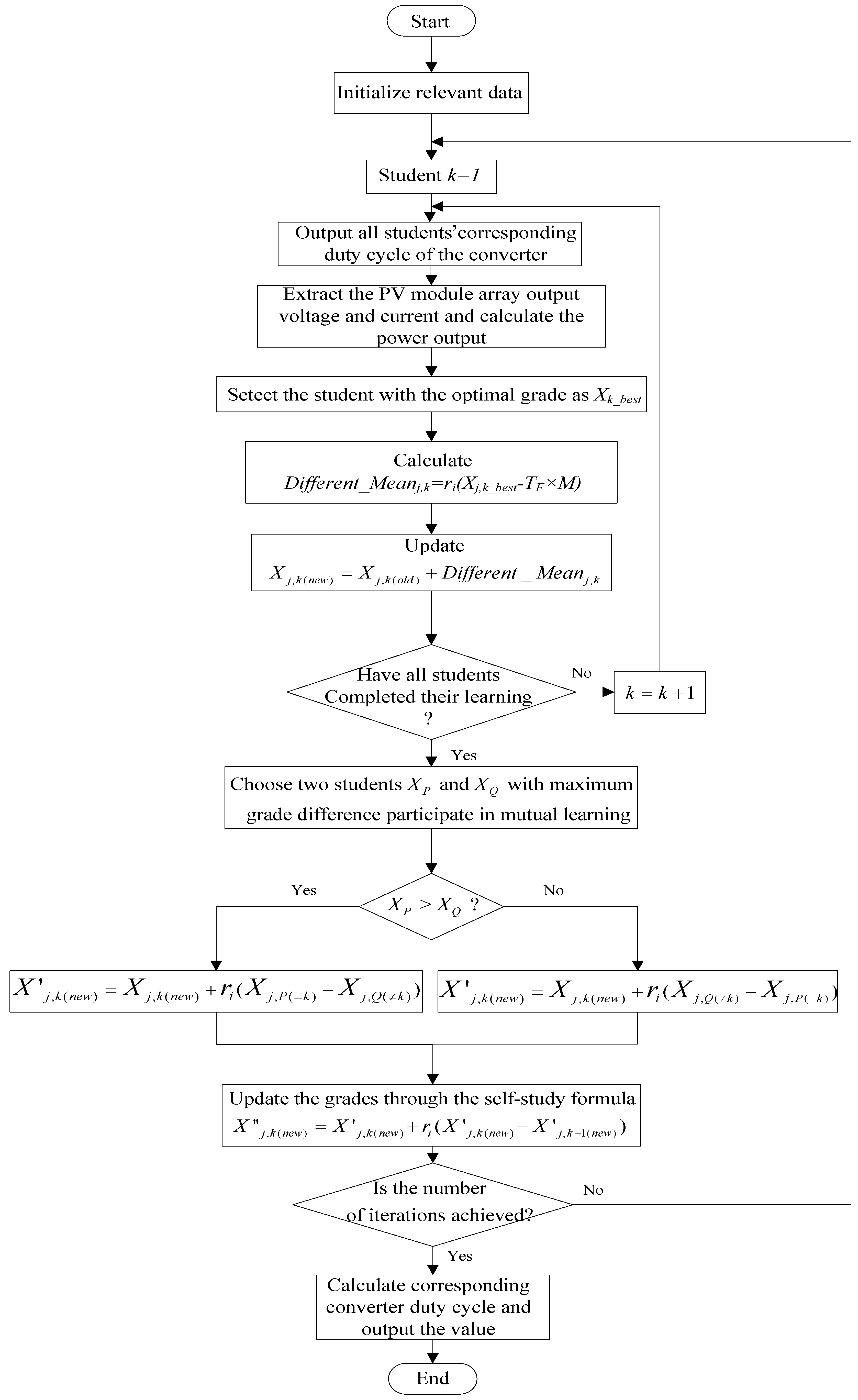
To address these problems, the present study incorporated a novel teaching-learning-based optimization (TLBO) method [23,24] to track the MPPs of a PV module array subjected to partial shading. The proposed method is advantageous because of its independence from population optimization, high adaptability, few design parameters, simple algorithm, and ease of understanding. In the present study, a conventional TLBO algorithm [25] was modified to improve the convergence and reduce the tracking time to obtain a more efficient algorithm than extant MPPT algorithms. The proposed algorithm improves MPPT tracking effectiveness for PV module arrays exhibiting multiple peaks in their P–V characteristic curves.

2. Fault and Shading Characteristics of PV Module Arrays

To increase the power output of a PV power generation system, PV modules are generally combined in serial and parallel configurations. However, external environments can cause shading because of dust, stains, and tall buildings, which generates nonlinear changes and multiple peaks in P–V characteristic curves. To examine the P–V and I–V output characteristics of serial and parallel PV module arrays subjected to partial shading, the SANYO HIP 2717 module [26] was adopted and various shading ratios were used. In addition, various arrays of serial and parallel configurations were tested.

Table 1. Electricity parameter specifications of the SANYO HIP 2717 PV module.

Parameter	Value
Rated maximum power output (Pmp)	27.8 W
MPP current (Imp)	1.63 A
MPP voltage (Vmp)	17.1 V
Short-circuit current (Isc)	1.82 A
Open-circuit voltage (Voc)	21.6 V
Module dimensions	496 mm × 524 mm

lists the electricity parameter specifications of a single module under standard test conditions (i.e., air mass of 1.5, irradiance of 1000 W/m², and PV module temperature of 25 °C) [26].

2.1. PV Module Simulator Circuit

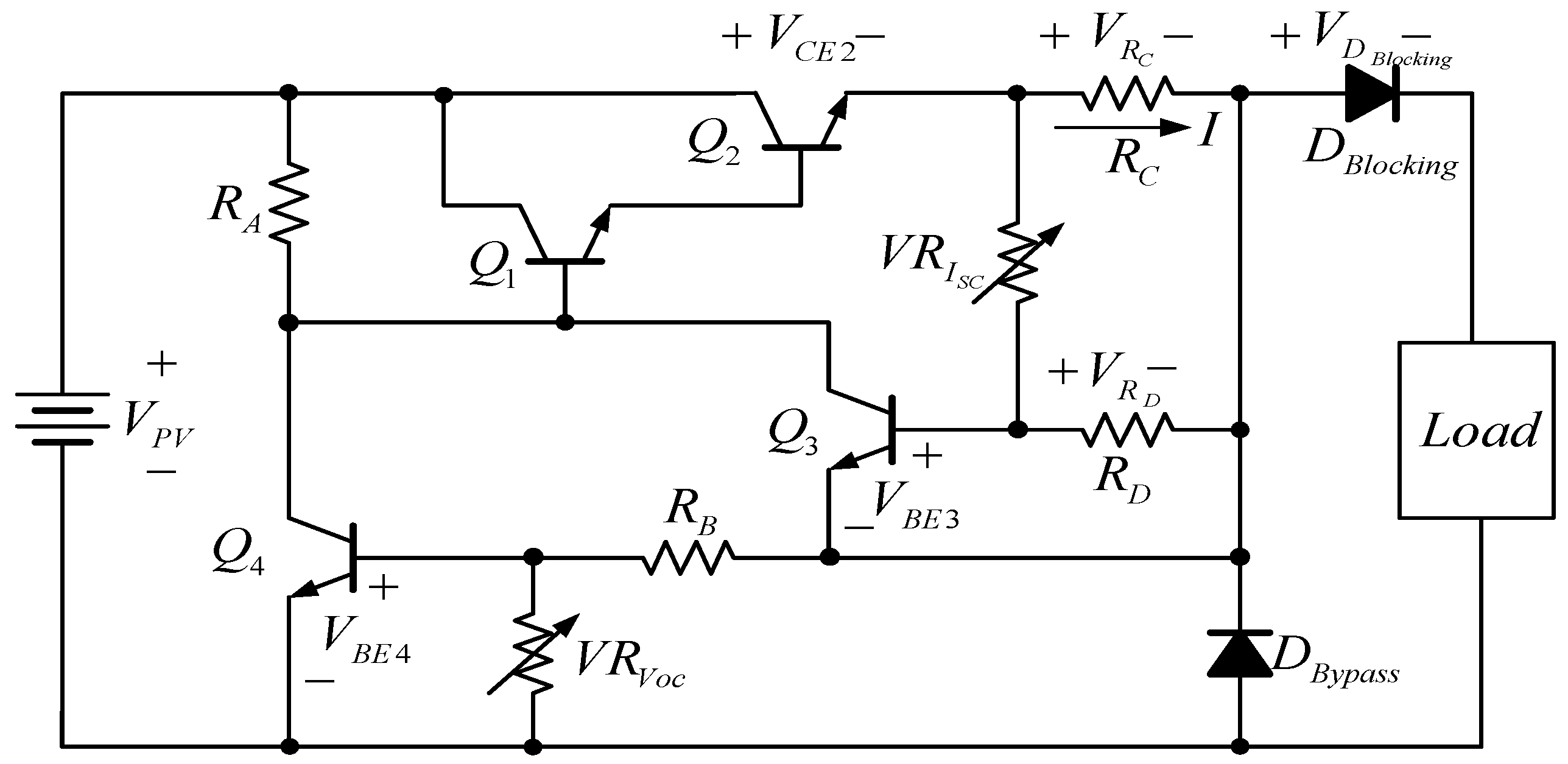
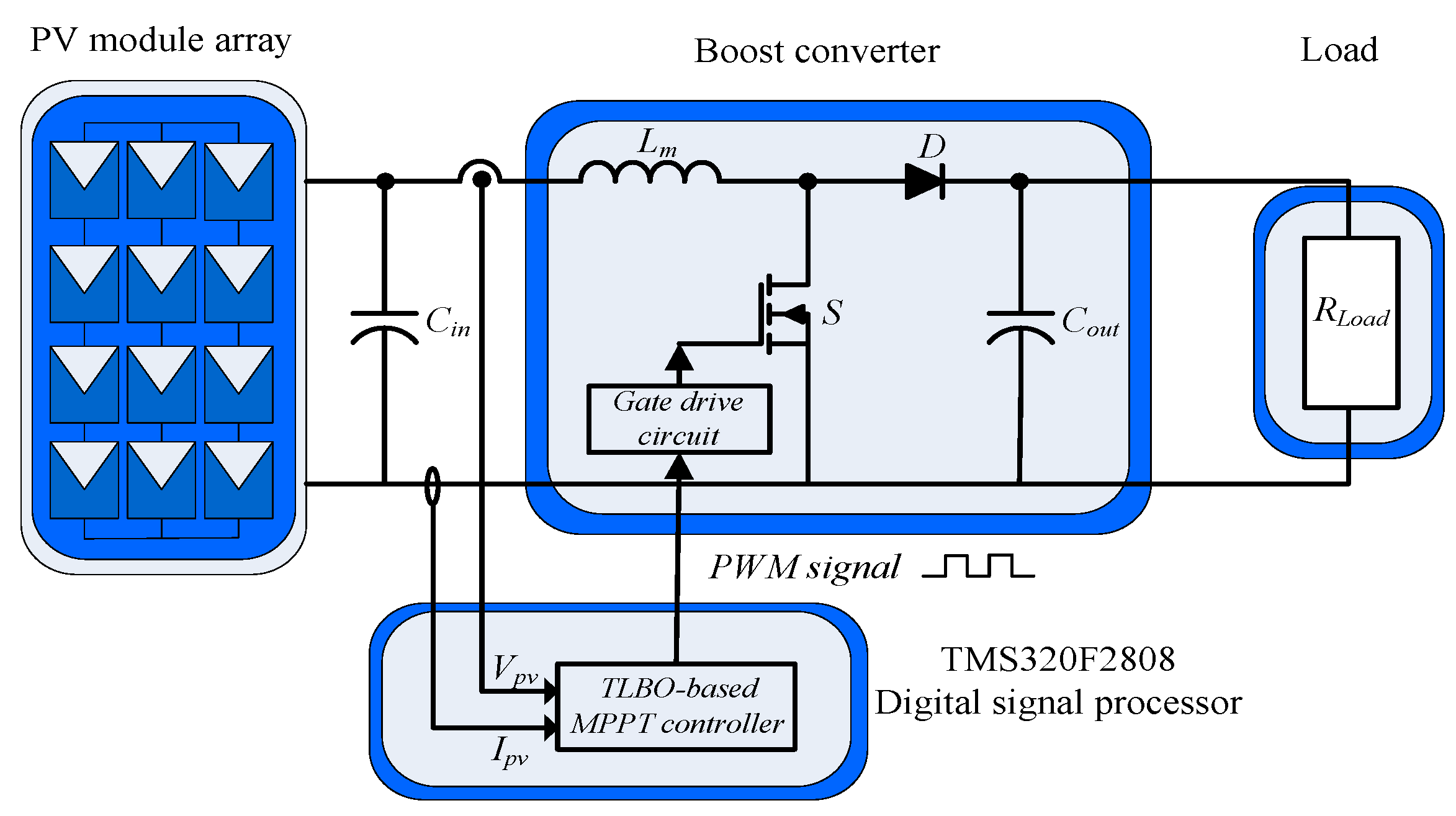
The present study adopted the circuit of a PV module simulator with adjustable shading ratios [27], as shown in Figure 1. The circuit structure primarily comprises a Darlington amplifier, a current limiting circuit, and a voltage regulator for attaining PV module output characteristics under varying shading ratios, which were created by adjusting variable resistors VR_Isc and VR_Voc. The variable resistor VR_Voc shown in Figure 1 controls the open-circuit voltage of the PV module. When the circuit is open, a current-limiting transistor Q₃ is operated at the cutoff region. The open-circuit voltage is calculated using Equation (1):

$$V_{oc}=V_{PV}-V_{CE2}-V_{D_{Blocking}}$$

(1)

Short-circuit currents can be calculated by adjusting VR_Isc to operate the current limiting transistor Q₃ at the saturation region when the V_BE3 voltage drop crosses over R_D. The short-circuit current is calculated using Equation (2):

$$I_{sc}=I=V_{BE3}\times \frac{R_D+V{R}_{ISC}}{R_D\times R_C}$$

(2)

If the V_PV power source is not provided, the PV module simulator generates zero power output, which is equivalent to the fault situation of the PV module. Using a bypass diode D_Bypass can ensure that PV module arrays generate a certain amount of power during fault events. Accordingly, the electricity parameters of PV modules can be employed to set the required PV module output characteristics.

2.2. PV Module Array Fault and Shading Characteristics Analysis

2.2.1. PV Module Array Characteristics without Faults or Shading

When a PV module array has M serial and N parallel arrays without shading or faults and the MPP voltage, MPP current, and MPP power are respectively denoted as V_mp, I_mp, and P_mp, the MPP voltage, MPP current, and MPP power of the M serial and N parallel arrays are expressed as M × V_mp, N × I_mp, and M × N × P_mp, respectively.

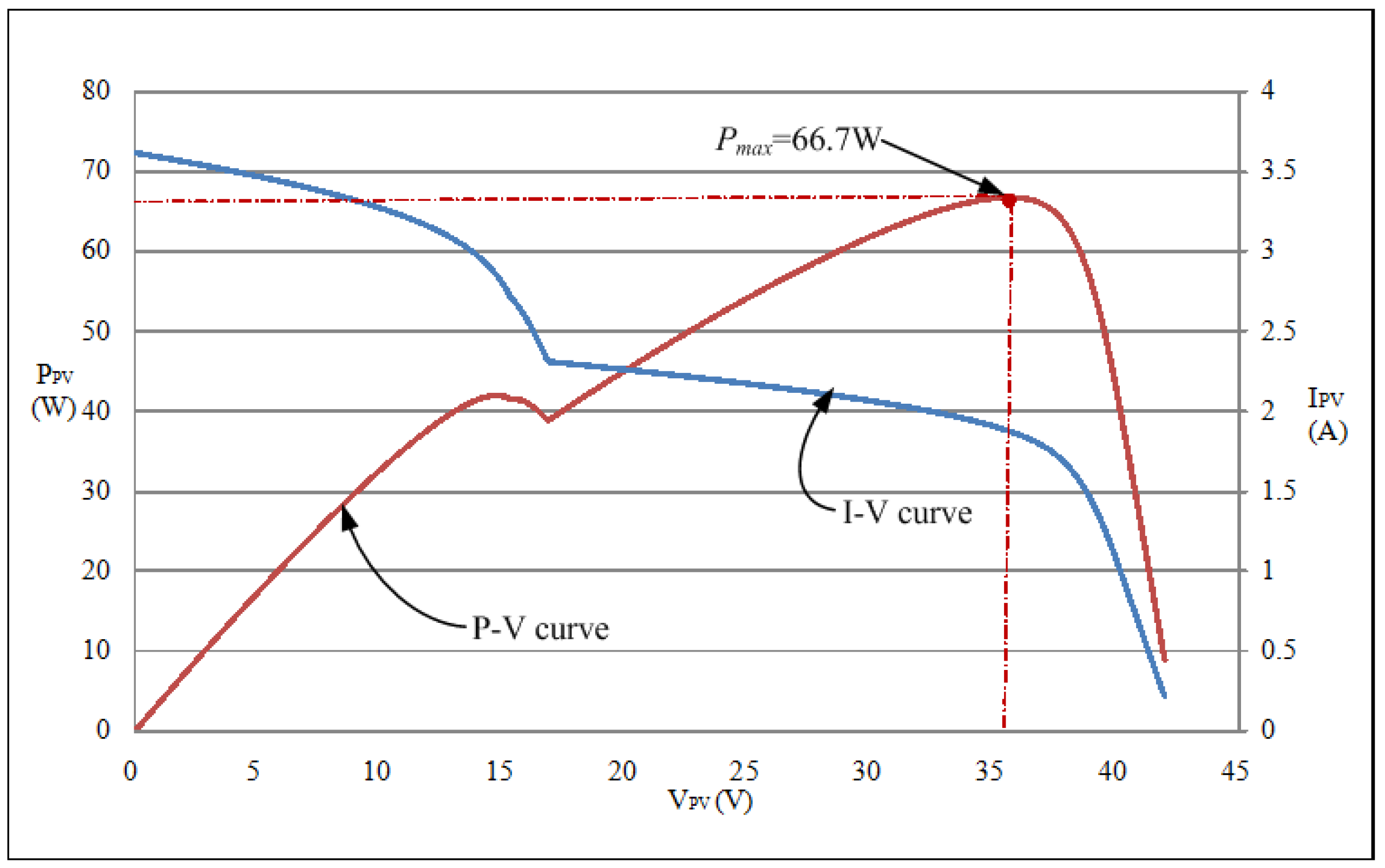
2.2.2. PV Module Array Characteristics with Faults or Shading

In a PV module array, fault or shading incidences in a module can decrease the power output of the array. Similar to an actual module, a PV module simulator enables a fault module to form a loop through a bypass diode. Using a bypass diode not only ensures that the PV module array maintains a certain level of power generation, but that it also has little effect on the MPPT. However, when the module is under partial shading, the output voltage and current decrease, causing multiple peaks in the P–V characteristic curves of the PV module array, which prevents conventional MPP trackers from controlling the module array to operate at the actual MPPs.

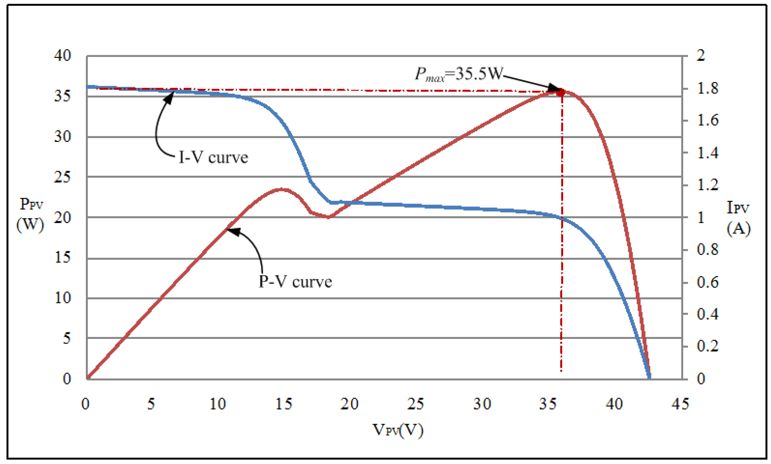
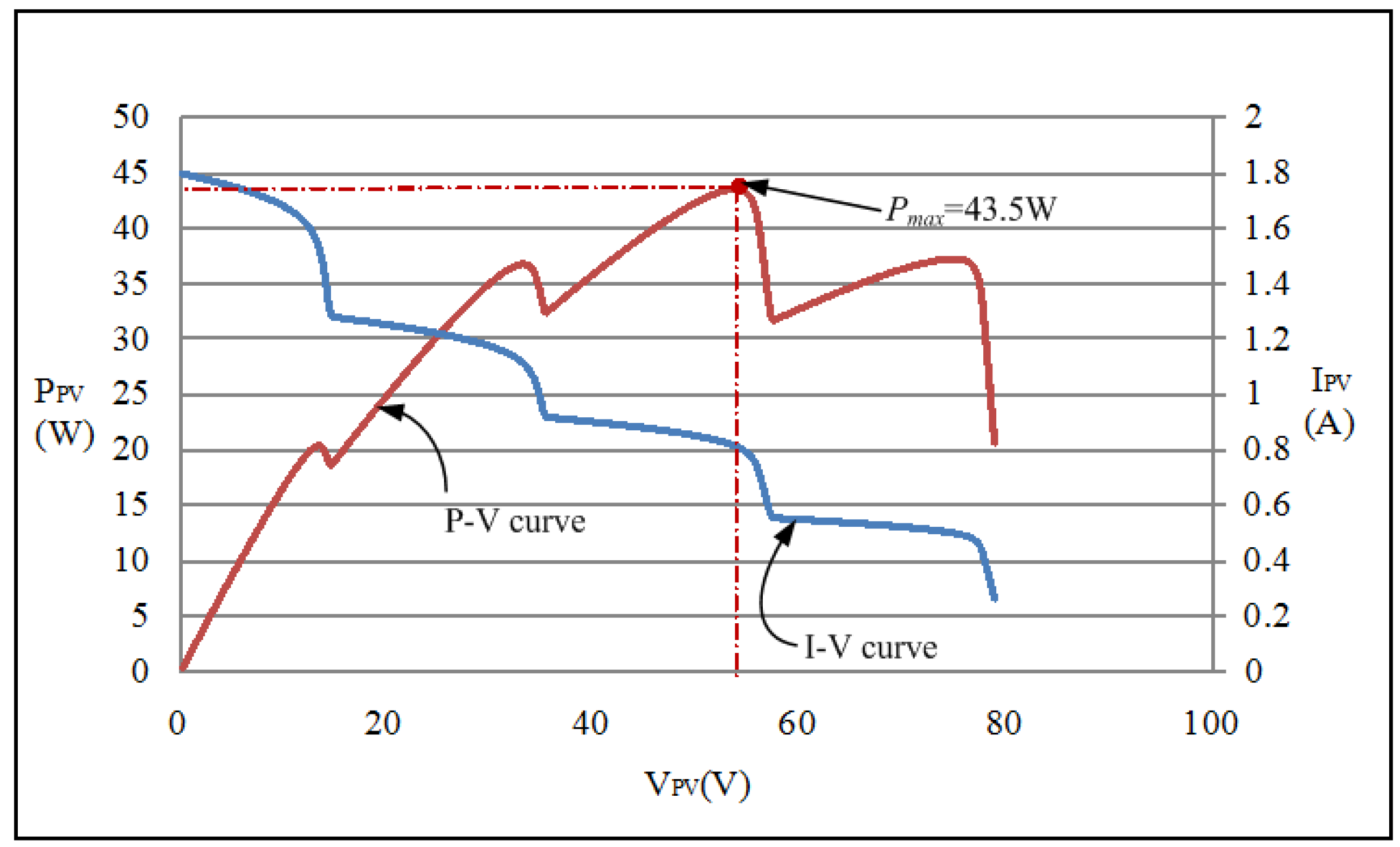
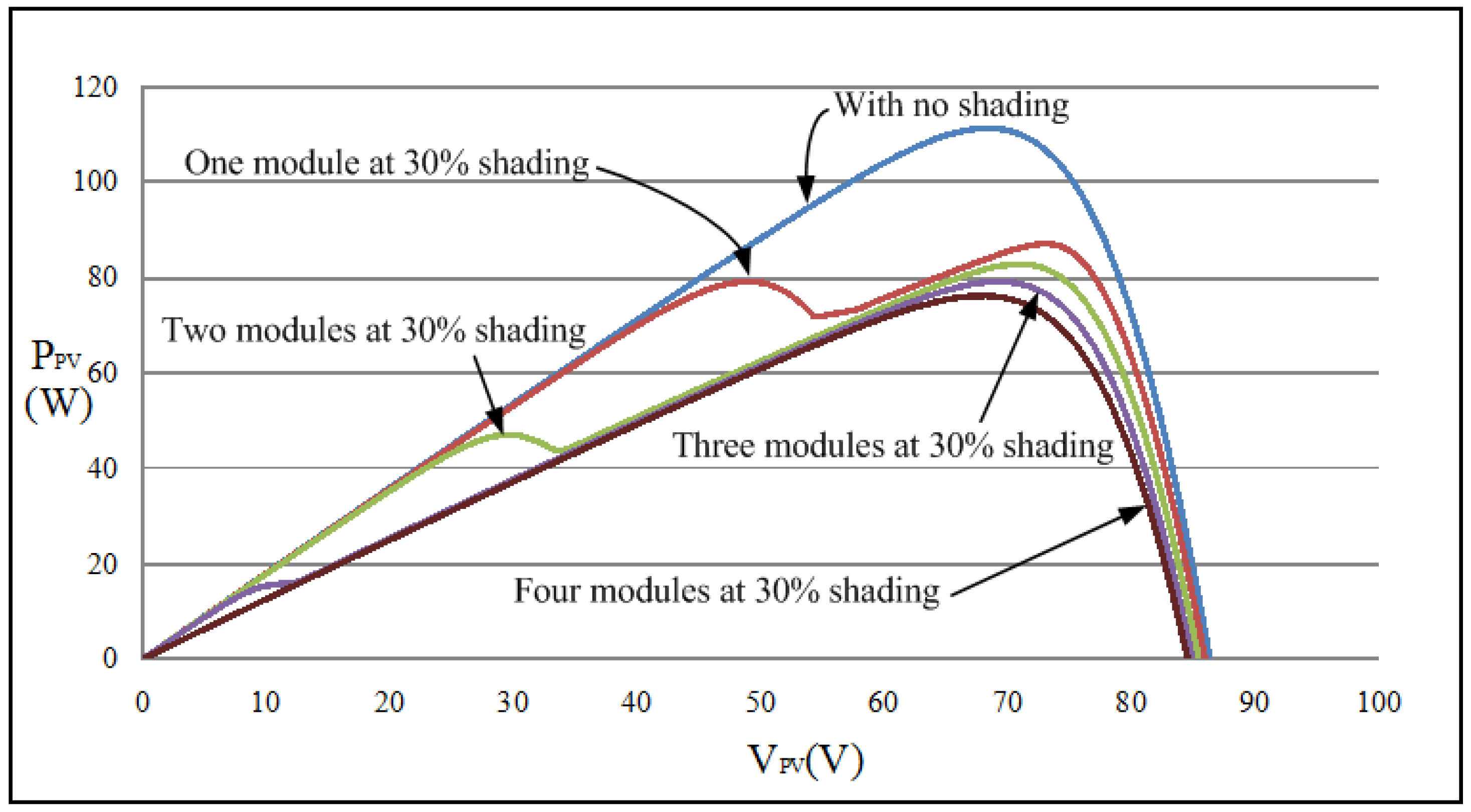
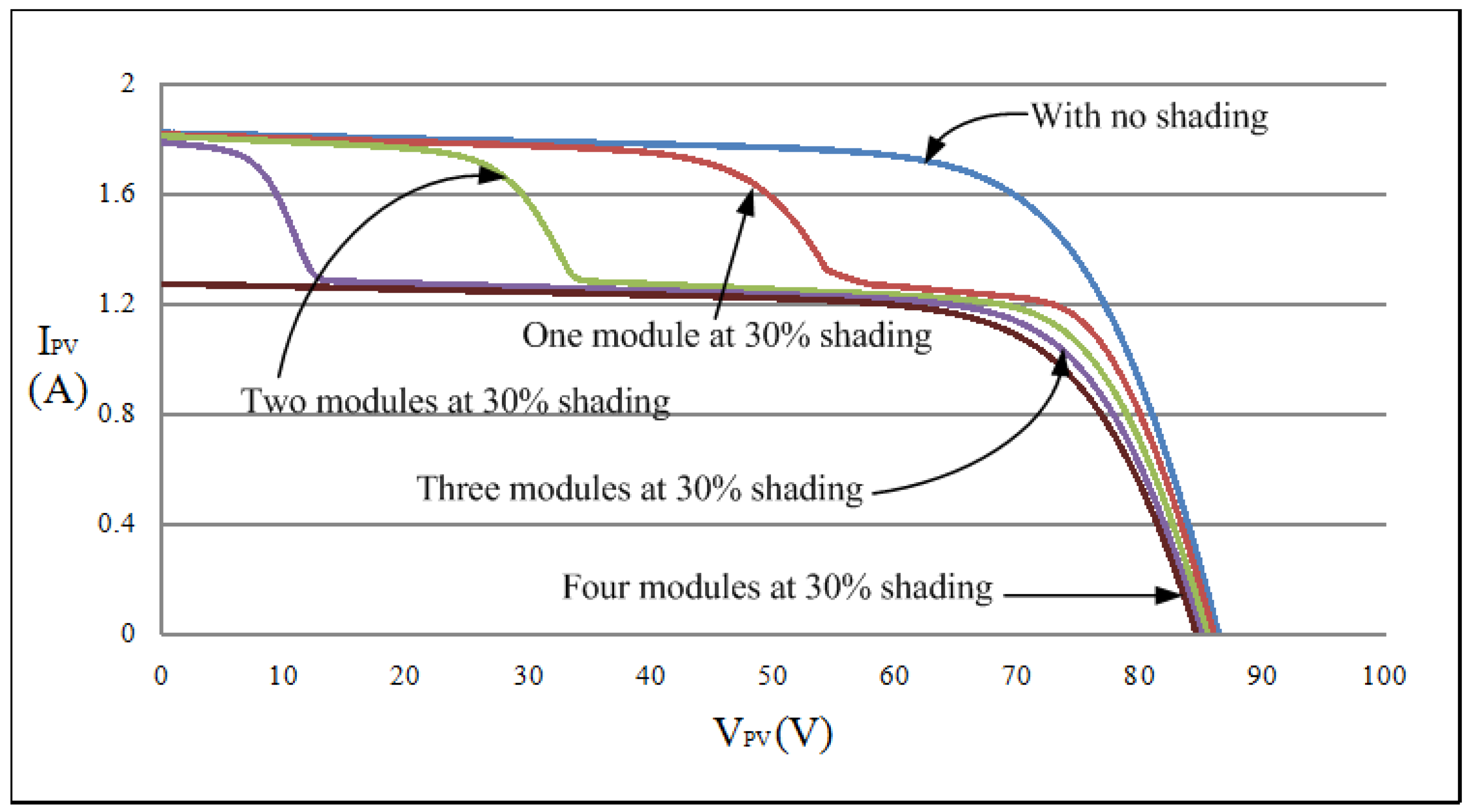
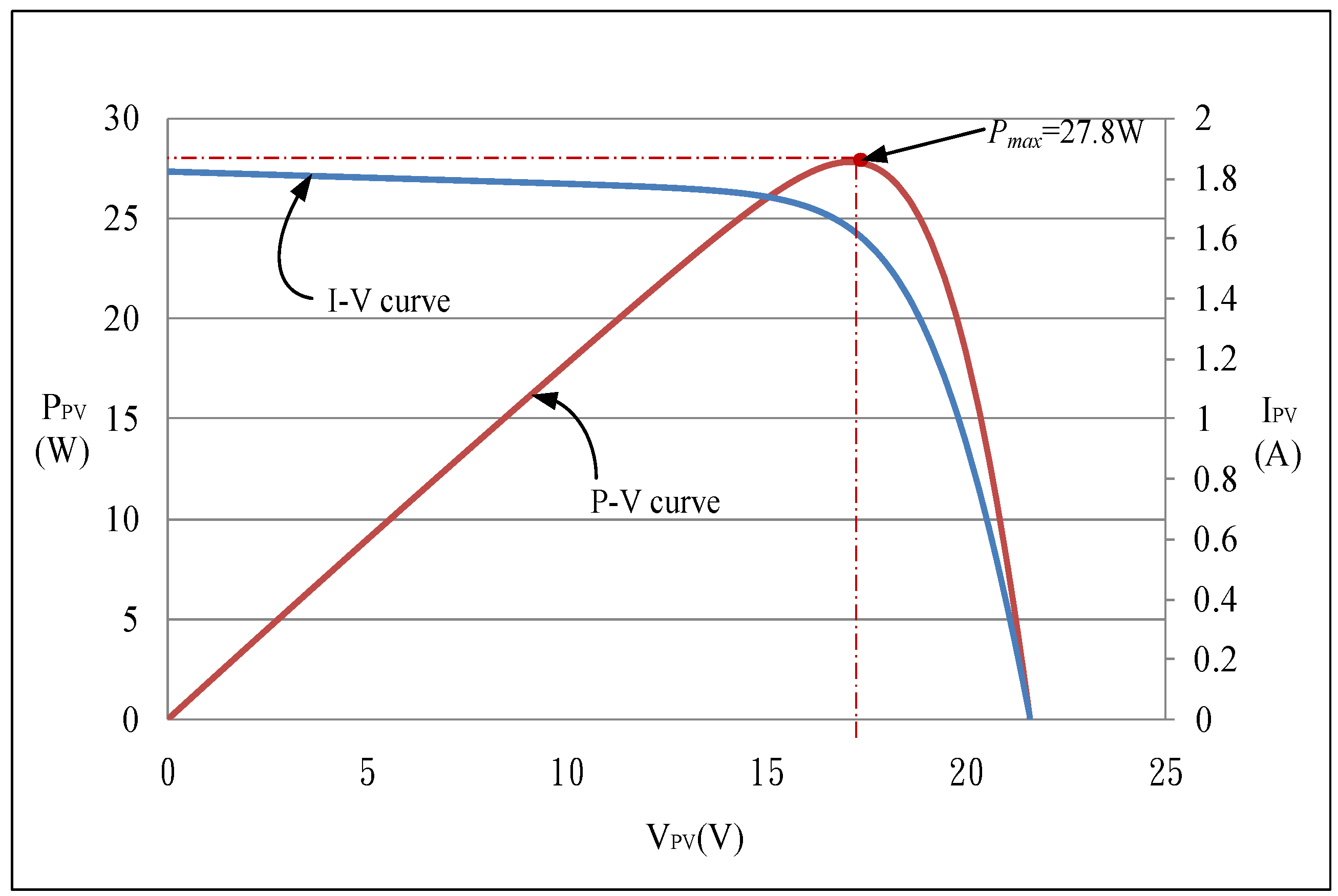
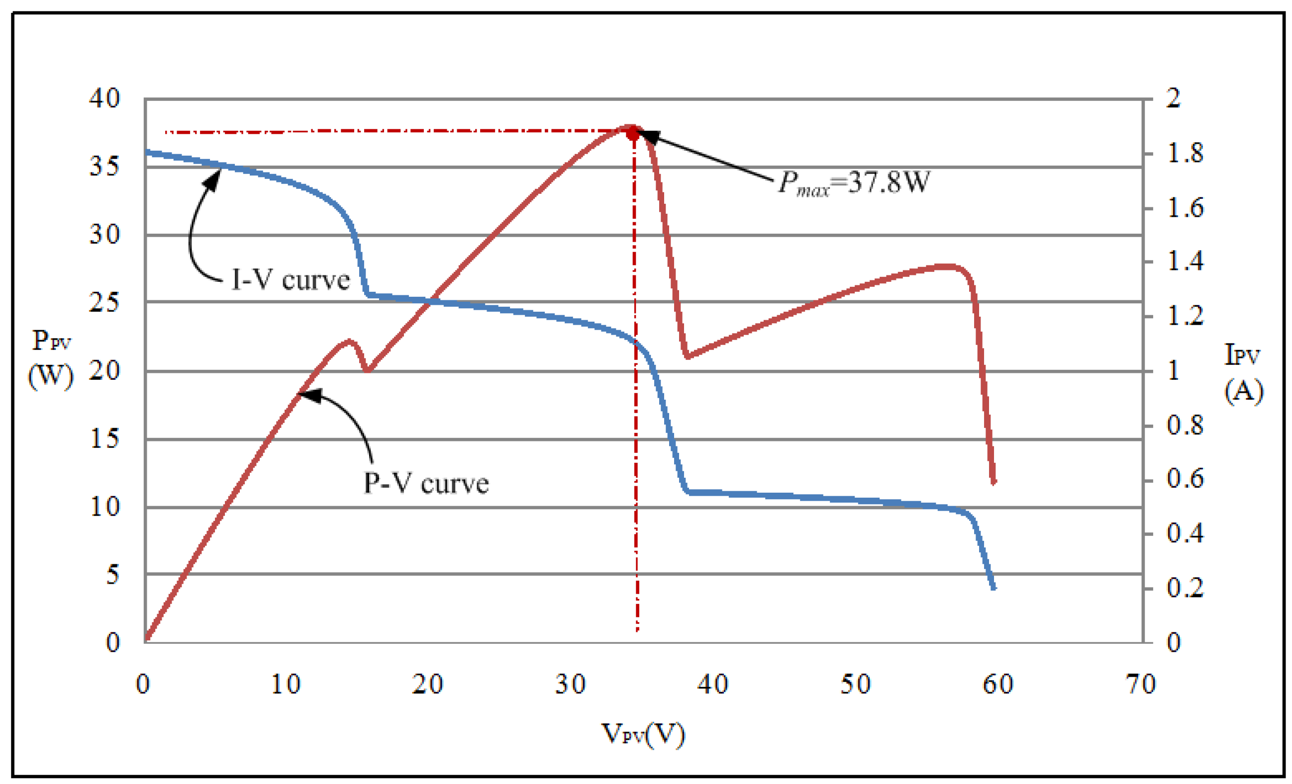
Given the aforementioned features of PV module arrays, the SANYO HIP 2717 module simulator was used to compose PV module arrays with different serial and parallel configurations under distinct shading ratios to perform a MPPT test. As shown in Figure 2 and Figure 3, SANYO HIP 2717 PV modules, built using the Solar Pro software [28], were adopted to compose a four-serial and one-parallel array. The P–V characteristic curves of an array with different numbers of muddles under a shading ratio of 30% were simulated. According to Figure 2 and Figure 3, partial shading of the modules in the array resulted in multiple peaks on the P–V characteristic curves, and the maximum power point (MPP) decreased with an increase in the number of modules under shading.

3. Teaching-Learning-Based Optimization (TLBO) Method

TLBO was proposed by Rao, Savsani, and Vakharia [29] in 2011. The concept of TLBO is to simulate the learning process between a teacher and students, the aim of which is to improve the grades of the entire class through teacher instruction and mutual learning between students. The students are comparable to individuals in an evolutionary algorithm and the teacher represents the optimal individual according to the fitness values.

3.1. Conventional TLBO Method

The steps of the traditional TLBO algorithm are as follows:

Step 1:

Set the values for the number of students N_p, subjects m, and iterations E.

Step 2:

Initialize a class S and define the following parameters:

(a)

Random student: $X_k\subset \{X_1,X_2,X_3,\dots ,X_{N_P}\}$

(b)

Random subject: $X_j\subset \{X_1,X_2,X_3,\dots ,X_m\}$

(c)

Target grade of student k in subject j: $G_{j,k}$

Step 3:

In the teaching phase, learning step r_i, teaching factor T_F, and students with the highest grades X_{j,k_best} are given. The mean of a class is calculated according to Equation (3) and substituted into Equation (4) to determine the student mean difference value. Finally, student grades are updated according to Equation (5) to identify the new target grade for each student in the teaching phase:

$$M={\displaystyle \sum _{k=1}^{N_P}\frac{X_k}{N_P}}$$

(3)

$$\begin{array}{cc}Different\_Mea{n}_{j,k}=r_i(X_{j,k\_best}-T_F\times M)& i=1,2,\dots ,E\end{array}$$

(4)

$$X_{j,k(new)}=X_{j,k(old)}+Different\_Mea{n}_{j,k}$$

(5)

Step 4:

In the learning phase, we assume that two random students X_P and X_Q participate in mutual learning, in which the student with the lower grade learns from the one with a higher grade. Adjustments were made using Equation (6):

$$\begin{array}{c}{X^{\prime }}_{j,k(new)}=X_{j,k(new)}+\left\{\begin{array}{c}ri(X_{j,P(=k)}-X_{j,Q(\ne k)}\\ ri(X_{j,Q(=k)}-X_{j,P(\ne k)}\end{array}\right\} \begin{array}{c}, if X_{j,P}>X_{j,Q}\\ , if X_{j,Q}>X_{j,P}\end{array}\\ X_P,X_Q\subset \left\{X_1,X_2,X_3,\dots ,X_{N_P}\right\}\end{array}$$

(6)

Step 5:

Repeat steps 3 and 4 until the iteration is completed.

Parameters used in conventional TLBO are explained as follows:

• Number of students (N_p): Total number of participating students.
• Number of iterations (E): Number of teaching and learning phases that the students experience.
• Subject grade (X_j,k): Grade of student k in subject j. Five subjects were used in the present study.
• Class mean (M): Mean grade of the class.
• Teaching step (r_i): Parameter for diversifying the student mean difference with a random value between 0 and 1.
• Teaching factor (T_F): Teachers’ ability to teach the students. The parameter randomly generates a value of 1 or 2.

In conventional TLBO, the teaching factors (T_F) used in the teaching phase generally comprise two fixed teaching capabilities (1 or 2). However, in real teaching situations, students’ levels differ and their learning capacity varies. Using fixed teaching factors may reduce learning effectiveness. In addition, learning from others (chosen at random) without conforming to students’ individual learning levels might not optimize their learning effectiveness. Thus, this study proposes an improved TLBO (I-TLBO) to solve the problems with conventional TLBO.

3.2. The Proposed I-TLBO Method

In the proposed I-TLBO, Steps 3 and 4 in conventional TLBO are modified through the following three improvements:

• Modification 1: The teaching factors T_F were modified to be automatically adjustable according to the students’ learning capacity. The adjustment method is expressed in Equation (7):

  $$T_F=\frac{X_{j,k}}{X_{j,k\_best}}$$

  (7)
• Modification 2: In the learning phase, a student selects another student who could benefit their learning the most in order to boost their learning effectiveness.
• Modification 3: A self-study process was incorporated into the learning phase to enable each student to adjust their self-learning according to their previous experience, as expressed in Equation (8):

  $$\begin{array}{cc}{X^{″}}_{j,k(new)}={X^{\prime }}_{j,k(new)}+r_i({X^{\prime }}_{j,k(new)}-{X^{\prime }}_{j,k-1(new)})& i=1,2,\dots ,E\end{array}$$

  (8)

In Equation (4), if X_{j,k_best} and M remain unchanged, then Different_Mean_j,k increases as T_F decreases. According to the actual MPPT process of PV module arrays, the tracking increment is directly proportional to the distance between the individual student grades and the MPP. Therefore, if the student grades in Improvement 1 are X₁ (i.e., power value P₁) and X′₁ (i.e., power value P′₁), then the teaching factors T_F of the student with the highest grades among all the students X_{j,k_best} (i.e., MPP value tracked so far P_{k_best}) are modified using Equations (9) and (10):

$$T_{F1}=\frac{P_1}{P_{k\_best}}$$

(9)

$$T_{F2}=\frac{{P^{\prime }}_1}{P_{k\_best}}$$

(10)

As depicted in Figure 4, the T_F1 value decreases as the Different_Mean value increases when student grade is distant from the MPP (e.g., X₁ position), thereby increasing the number of tracking steps needed to approach the maximum value rapidly. By contrast, when the student grade is close to the MPP (e.g., X′₁ position), the T_F2 value increases as the Different_Mean value and number of tracking steps decrease to approach the maximum value slowly. Thus, the students can adjust their tracking steps according to their learning capacity. In improvements 2 and 3, students can spontaneously learn from a student who is helpful to them. The term X′_j,k-1(new) represents the student’s previous learning abilities, which is used as a basis for the other student’s self-study. In summary, the self-learning method not only accelerates the learning progress, but also escapes local solutions and reaches global convergence. A flowchart of the proposed I-TLBO MPPT is shown in Figure 5.

3.3. MPP Tracker

Figure 6 depicts the MPP tracker architecture of the PV module array based on the proposed I-TLBO. The architecture mainly comprises two subsystems: a DC/DC boost converter and I-TLBO-based MPPT controller. When employed in a DC/DC boost converter, a synchronous rectification is known to outperform a diode rectification in terms of the conversion efficiency as well as the thermal performance [30], while a diode rectification is adopted instead in this work due to the reliability concern. As stated previously, the I-TLBO-based MPPT controller controls the duty cycle of the boost converter, enabling the PV module array to generate the maximum power output under partial shading.

Table 2. DC/DC boost converter component parameters.

Component	Model Number and Specifications
Inductance (Lm)	3.3 mH
Input capacitance (Cin)	220 μF/160 V
Output capacitance (Cout)	390 μF/450 V
Switching frequency (fs)	20 kHz
Power MOSFET (S)	IRF460 (500 V/20A)
Diode (D)	DSEP30-12A (1200 V/30A)

lists the DC/DC boost converter parameter settings [31] and

Table 3. Conventional TLBO parameter settings.

Parameter	Setting
Number of students (NP)	4
Number of iterations (E)	40
Teaching step (ri)	Random value between 0 and 1
Teaching factor (TF)	1 or 2

lists the conventional TLBO parameter settings. The component choices are made according to [31]. Without extra effort, components available in our laboratories but with over specified ratings, are directly taken to implement the DC/DC boost converter. In I-TLBO, the T_F in Table 3 is replaced with the parameter setting in

Table 4. I-TLBO Parameter Settings.

Parameter	Setting
Teaching factor (TF)	$T_F=\frac{X_{j,k}}{X_{j,k\_best}}$

whereas all other parameters remain unchanged. Subsequently, the PV module array was tested under five distinct operating situations, as shown in

Table 5. Cases of the five selected serial and parallel configurations and the shading situations.

Case	Serial and Parallel Configurations and Shading Situations	Number of Peaks in the P–V Characteristic Curves
1	One-serial and one-parallel with 0% shading	Single
2	Two-serial and one-parallel with 0% and 40% shading	Double
3	Three-serial and one-parallel with 0%, 40%, and 70% shading	Triple
4	Four-serial and one-parallel with 0%, 30% shading, 50%, and 70% shading	Quadruple
5	Two-serial and two-parallel with (30% and 0% shading)//(0% and 50% shading)	Double

Note: “//” parallel connection.

.

4. Measurement Results

The PV module simulator circuit in Figure 1 was employed to compose the module array configurations under five operating situations as listed in Table 5. The P–V and I–V characteristic curves of PV module arrays under different shading ratios were measured using an MP 170 I–V checker by EKO Instruments CO. Ltd (Tokyo, Japan). The aim is to tell whether the global MPPs in the 5 testing cases listed in Table 5 can be tracked as expected using I-TBLO MPPT. Subsequently, a digital signal processor TMS320F2808 [32] was used to perform MPPT by using conventional TLBO and the proposed I-TLBO. The tracking performance of the two methods was also compared.

4.1. PV Module Array Characteristics under Different Operating Situations

Figure 7, Figure 8, Figure 9, Figure 10 and Figure 11 depict the I–V and P–V characteristic curves of the PV module arrays under the five operating situations listed in Table 5. Figure 7 shows the output characteristics of a single PV module. The output characteristic curve reveals that the parameters related to the output characteristics of modules not affected by shading or faults are identical to the electricity parameter specifications listed in Table 1. The module in Figure 7 was used as a basis for testing the serial configurations (i.e., Cases 1–4) as well as the serial and parallel configurations (Case 5), as listed in Table 5. Different shading ratio conditions were set to produce multiple peaks in the characteristic curves to exemplify the exceptional performance of the proposed I-TLBO on MPPT. Figure 8, Figure 9 and Figure 10 reveal that double, triple, and quadruple peaks occur in Cases 2 to 4. Thus, we inferred that N peaks would appear in P–V characteristic curves when N modules in a serial array were under different shading ratios. Figure 11 shows the I–V and P–V characteristic curves measured on the two-serial and two-parallel configuration module array of Case 5. Although two modules in each serial module were subjected to different shading ratios, the parallel connection between the two-serial modules generated double peaks only in the P–V characteristic curve.

4.2. MPPT Measurement of PV Module Arrays

The measurement architecture is shown in Figure 6. First, the output voltage V_PV and current I_PV of the PV module arrays were extracted through sensors and signal conversion circuits and entered into the TMS320F2808 digital signal processor. Subsequently, TLBO was applied to perform MPPT. The resulting optimal duty cycle trigger signal was sent to the boost converter to control the on time of power transistors, thereby controlling the maximum power output of the PV module array.

Figure 12, Figure 13, Figure 14, Figure 15 and Figure 16 show the waveforms of output voltage V_PV and current I_PV measured on the PV module arrays. The power curves are demonstrated as the product of voltage and current through the internal computation functions of the oscilloscope. In the 40th iteration, the quality of the conventional TLBO and the proposed I-TLBO tracking response speed were observed and compared when the power curve approached a stable value.

4.2.1. Case 1 (One-Serial and One-Parallel: 0% Shading)

Figure 12a,b depict the MPPT waveforms of Case 1 (0% shading) measured by using the conventional TLBO and the proposed I-TLBO, respectively. The results revealed that under standard test conditions, the output characteristics of the PV module simulator were identical to the electricity parameter specifications in Table 1. In addition, the tracking time between time points t₀ and t₁ in Figure 12 showed that the proposed I-TLBO (2.5 s) converged faster than did conventional TLBO (3.5 s).

4.2.2. Case 2 (Two-Serial and One-Parallel: 0% and 40% Shading)

Figure 13a,b depict the MPPT waveforms of Case 2 measured by using conventional TLBO and the proposed I-TLBO, respectively. The two-serial and one-parallel configuration was composed on the basis of the single module of Case 1. One module in Case 2 was under 40% shading. The empirical results revealed that under partial shading, the PV module array generated a double-peaked P–V characteristic curve (Figure 8). Although both the conventional and proposed methods tracked the actual MPP, the proposed I-TLBO (2.4 s) was faster than conventional TLBO (2.7 s) in MPPT response speed.

4.2.3. Case 3 (Three-Serial and One-Parallel: 0%, 30%, and 70% Shading)

Figure 14a,b depict the MPPT waveforms Case 3 measured by using conventional TLBO and the proposed I-TLBO, respectively. The empirical results revealed that three modules under different shading ratios generated triple peaks in the P–V characteristic curve and a long tracking time under conventional TLBO (3.4 s). By contrast, the proposed I-TLBO (2.7 s) tracked the real MPPT in less time.

4.2.4. Case 4 (Four-Serial and One-Parallel: 0%, 30%, 50%, and 70% Shading)

Figure 15a,b show the MPPT waveforms of Case 4 measured by using conventional TLBO and the proposed I-TLBO, respectively. The empirical results revealed that the proposed I-TLBO required only 2.2 s, whereas conventional TLBO required 3.4 s of tracking time (t₀ to t₁) to track the MPP. This validates that the proposed I-TLBO outperformed conventional TLBO in tracking.

4.2.5. Case 5 (Two-Serial and Two-Parallel: (0% and 30% Shading)//(0% and 50% Shading))

Figure 16a,b show the MPPT waveforms of Case 5 measured by using conventional TLBO and the proposed I-TLBO, respectively. The empirical results revealed that adopting the random teaching factor T_F in conventional TLBO slowed the MPPT. By contrast, the proposed I-TLBO identified the real MPP within a short time (3.5 s).

4.2.6. Comparison of the Case Measurements

Table 6. Comparison between the measurement results of the five cases obtained using ACO, PSO, conventional TLBO and the proposed I-TLBO.

Case	P–V Curve Peaks	ACO [17]		PSO [21]		Conventional TLBO		Proposed I-TLBO
		Average Tracking Time	Average MPP	Average Tracking Time	Average MPP	Average Tracking Time	Average MPP	Average Tracking Time	Average MPP
1	Single	4.3 s	27.5 W	3.4 s	27.3 W	3.3 s	27.0 W	2.5 s	27.8 W
2	Double	4.8 s	35.3 W	3.0 s	35.0 W	2.8 s	35.1 W	2.4 s	35.8 W
3	Triple	5.1 s	37.5 W	3.8 s	37.0 W	3.4 s	37.2 W	2.7 s	38.5 W
4	Quadrupe	5.6 s	43.2 W	Tracking failed	35.7 W	3.6 s	43.0 W	2.2 s	43.4 W
5	Double	5.8 s	66.3 W	5.2 s	64.7 W	4.8 s	66.1 W	3.7 s	66.7 W

gives the performance comparison in terms of the average tracking time and the average MPP for 40 iterations among the proposed I-TBLO, a typical TLBO, ACO [17] and PSO [21], both referred to in the Introduction section. This proposal is obviously found to outperform the counterparts in terms of dynamic tracking response and static performance for the five cases investigated in the present study underwent MPPT.

5. Conclusions

In this study, an I-TLBO was proposed to perform MPPT of PV module arrays. To enhance the TLBO tracking efficiency and performance, an intellectual teaching factor adjustment method was adopted to facilitate automatic adjustments of TLBO teaching factors. In addition, in the learning phase, the students automatically tracked the targets benefiting their learning. Eventually, each student expedited their tracking speed through self-study according to their individual experience. The empirical results verified that the proposed I-TLBO can more rapidly identify the real MPP compared with conventional TLBO, ACO and PSO when certain modules in a PV module array are under partial shading. The results of the measurements of the designed five cases of shading confirmed that the proposed I-TLBO tracked the global MPP within a shorter period than conventional TLBO, ACO and PSO can. These results confirm the feasibility of applying the proposed I-TLBO in PV module array MPPT, particularly in situations where multiple peaks occur on the P–V characteristic curves because of partial shading. This proposed high performance tracking algorithm can be also directly applied to track the MPP for each single PV module using a DC/DC converter, and to track the MPP on a one-peak P–V curve using a central inverter.

References

1. Wang, X.; Liang, H. Output characteristics of PV array under different insolation and temperature. In Proceedings of the IEEE 2012 Conference on Asia Pacific Power and Energy Engineering (APPEE), Shanghai, China, 27–29 March 2012; pp. 1–4.
2. Femia, N.; Granozio, D.; Petrone, G.; Spagnuolo, G.; Vitelli, M. Predictive and adaptive MPPT perturb and observe method. IEEE Trans. Aerosp. Electron. Syst. 2007, 43, 934–950. [Google Scholar] [CrossRef]
3. Luigi, P.; Renato, R.; Ivan, S.; Pietro, T. Optimized adaptive perturb and observe maximum power point tracking control for photovoltaic generation. Energies 2015, 8, 3418–3436. [Google Scholar] [CrossRef]
4. D’Souza, N.S.; Lopes, L.A.C.; Liu, X. Comparative study of variable size perturbation and observation maximum power point trackers for PV systems. Electr. Power Syst. Res. 2010, 80, 296–305. [Google Scholar] [CrossRef]
5. Lin, C.H.; Huang, C.H.; Du, Y.C.; Chen, J.L. Maximum photovoltaic power tracking for the PV array using the fractional-order incremental conductance method. Appl. Energy 2011, 88, 4840–4847. [Google Scholar] [CrossRef]
6. Li, C.; Chen, Y.; Zhou, D.; Liu, J.; Zeng, J. A high-performance adaptive incremental conductance MPPT algorithm for photovoltaic systems. Energies 2016, 9, 288–305. [Google Scholar] [CrossRef]
7. Mohammadmehdi, S.; Saad, M.; Rasoul, R.; Rubiyah, Y.; Ehsan, T.R. Analytical modeling of partially shaded photovoltaic systems. Energies 2013, 6, 128–144. [Google Scholar] [CrossRef] [Green Version]
8. Balato, M.; Vitelli, M.; Femia, N.; Petrone, G.; Spagnuolo, G. Factors limiting the efficiency of DMPPT in PV applications. In Proceedings of the International Conference on Clean Electrical Power, Ischia, Italy, 14–16 June 2011; pp. 604–608.
9. Vitelli, M. On the necessity of joint adoption of both distributed maximum power point tracking and central maximum power point tracking in PV systems. Prog. Photovolt. Res. Appl. 2014, 22, 283–299. [Google Scholar] [CrossRef]
10. Iacca, G.; Mallipeddi, R.; Mininno, E.; Neri, F.; Suganthan, P.N. Global supervision for compact differential evolution. In Proceedings of the 2011 IEEE Symposium on Differential Evolution (SDE), Paris, France, 11–15 April 2011; pp. 1–8.
11. Dorigo, M.; Birattari, M.; Stutzle, T. Ant colony optimization. IEEE Comput. Intell. Mag. 2006, 1, 28–39. [Google Scholar] [CrossRef]
12. Gao, W.; Liu, S.; Huang, L. A global best artificial bee colony algorithm for global optimization. J. Comput. Appl. Math. 2012, 236, 2741–2753. [Google Scholar] [CrossRef]
13. Hadji, S.; Gaubert, J.P.; Krim, F. Genetic algorithms for maximum power point tracking in photovoltaic systems. In Proceedings of the IEEE 2011—14th European Conference on Power Electronics and Applications (EPE), Birmingham, UK, 30 August–1 September 2011; pp. 1–9.
14. Hadji, S.; Gaubert, J.P.; Krim, F. Experimental analysis of genetic algorithms based MPPT for PV systems. In Proceedings of the IEEE Conference on International Renewable and Sustainable Energy (IRSEC), Ouarzazate, Morocco, 17–19 October 2014; pp. 7–12.
15. Tajuddin, M.F.N.; Ayob, S.M.; Salam, Z. Tracking of maximum power point in partial shading condition using differential evolution (DE). In Proceedings of the IEEE 2012 International Conference on Power and Energy (PECon), Kota Kinabalu, Malaysia, 2–5 December 2012; pp. 384–389.
16. Storn, R. On the usage of differential evolution for function optimization. In Proceedings of the Biennial Conference of the North American in Fuzzy Information Processing Society (NAFIPS), Berkeley, CA, USA, 19–22 June1996; pp. 519–523.
17. Lian, J.; Maskell, D.L. A uniform implementation scheme for evolutionary optimization algorithms and the experimental implementation of an ACO based MPPT for PV systems under partial shading. In Proceedings of the IEEE Symposium on Computational Intelligence Applications in Smart Grid (CIASG), Orlando, FL, USA, 9–12 December 2014; pp. 1–8.
18. Sundareswaran, K.; Sankar, P.; Nayak, P.S.R.; Simon, S.P.; Palani, S. Enhanced energy output from a PV system under partial shaded conditions through artificial bee colony. IEEE Trans. Energy Convers. 2015, 6, 198–209. [Google Scholar] [CrossRef]
19. Lian, K.L.; Jhang, J.H.; Tian, I.S. A maximum power point tracking method based on perturb-and-observe combined with particle swarm optimization. IEEE J. Photovolt. 2014, 4, 626–633. [Google Scholar] [CrossRef]
20. Daraban, S.; Petreus, D.; Morel, C. A novel global MPPT based on genetic algorithms for photovoltaic systems under the influence of partial shading. In Proceedings of the IEEE 2013—39th Annual Conference on Industrial Electronics Society (IECON), Vienna, Austria, 10–13 November 2013; pp. 1490–1495.
21. Kashif, I.; Zainal, S.; Amir, S.; Muhammad, A. A direct control based maximum power point tracking method for photovoltaic system under partial shading conditions using particle swarm optimization algorithm. Appl. Energy 2012, 99, 414–422. [Google Scholar] [CrossRef]
22. Chao, K.H.; Lin, Y.S.; Lai, U.D. Improved particle swarm optimization for maximum power point tracking in photovoltaic module arrays. Appl. Energy 2015, 158, 609–618. [Google Scholar] [CrossRef]
23. Rao, R.V.; Savsani, V.J.; Vakharia, D.P. Teaching-learning-based optimization: A novel method for constrained mechanical design optimization problems. J. Comput. Aided Des. 2011, 43, 303–315. [Google Scholar] [CrossRef]
24. Satapathy, S.C.; Naik, A.; Parvathi, K. Weighted teaching-learning-based optimization for global function optimization. Appl. Math. Sci. Res. Publ. 2013, 4, 429–439. [Google Scholar] [CrossRef]
25. Rao, R.V.; Patel, V. An improved teaching-learning-based optimization Algorithm for solving unconstrained optimization problems. Comput. Sci. Eng. Electr. Eng. 2013, 20, 710–720. [Google Scholar] [CrossRef]
26. SANYO HIP 2717 Datasheet. Available online: http://iris.nyit.edu/~mbertome/solardecathlon/SDClerical/SD_DESIGN+DEVELOPMENT/091804_Sanyo190HITBrochure.pdf (accessed on 15 January 2016).
27. Chao, K.H.; Chao, Y.W.; Chen, J.P. A circuit-based photovoltaic module simulator with shadow and fault setting. Int. J. Electron. 2016, 103, 424–438. [Google Scholar] [CrossRef]
28. Solar Pro Official Website. Available online: http://lapsys.co.jp/english (accessed on 10 May 2016).
29. Rao, R.V.; Patel, V.; Chen, J.P. An elitist teaching-learning-based optimization algorithm for solving complex constrained optimization problems. Int. J. Ind. Eng. Comput. 2012, 3, 535–560. [Google Scholar] [CrossRef]
30. Graditi, G.; Adinolfi, G.; Femia, N.; Vitelli, M. Comparative analysis of synchronous rectification boost and diode rectification boost converter for DMPPT applications. In Proceedings of the 2011 IEEE International Symposium on Industrial Electronics (ISIE), Gdansk, Poland, 27–30 June 2011; pp. 1000–1005.
31. Hart, D.W. Introduction to Power Electronics; Prentice Hall: New York, NY, USA, 2003. [Google Scholar]
32. TMS320F2808 Data Sheet. Available online: http://www.ti.com/lit/ds/symlink/tms320f2808.pdf (accessed on 12 March 2016).
Figure 1. PV module simulator circuit.
Energies 09 00986 g001
Figure 2. Simulated P–V characteristic curves of the four-serial and one-parallel array with different numbers of modules under 30% shading.
Energies 09 00986 g002
Figure 3. Simulated I–V characteristic curves of the four-serial and one-parallel array with different numbers of modules under 30% shading.
Energies 09 00986 g003
Figure 4. Adjustment of teaching factors of the proposed I-TLBO.
Energies 09 00986 g004
Figure 5. MPPT flow chart of the proposed I-TLBO.
Energies 09 00986 g005
Figure 6. Architecture of the I-TLBO-based MPPT controller.
Energies 09 00986 g006
Figure 7. I–V and P–V characteristic curves of one-serial and one-parallel module array with 0% shading.
Energies 09 00986 g007
Figure 8. I–V and P–V characteristic curves of the two-serial and one-parallel module array with 0% and 40% shading.
Energies 09 00986 g008
Figure 9. I–V and P–V characteristic curves of the three-serial and one-parallel module array with 0%, 30%, and 70% shading.
Energies 09 00986 g009
Figure 10. I–V and P–V characteristic curves of the four-serial and one-parallel module array with 0%, 30%, 50%, and 70% shading.
Energies 09 00986 g010
Figure 11. I–V and P–V characteristic curves of the two-serial and two-parallel module array with [(0% and 30% shading)//(0% and 50% shading)].
Energies 09 00986 g011
Figure 12. Measurement results of the one-serial and one-parallel module array with 0% shading by using (a) conventional TLBO (Pmp = 27.4 W) and (b) the proposed I-TLBO (Pmp = 27.8 W).
Energies 09 00986 g012aEnergies 09 00986 g012b
Figure 13. Measurement results of the two-serial and one-parallel module array (0% and 40% shading) by using (a) conventional TLBO (Pmp = 35.1 W) and (b) the proposed I-TLBO (Pmp = 35.8 W).
Energies 09 00986 g013aEnergies 09 00986 g013b
Figure 14. Measurement results of the three-serial and one-parallel module array (0%, 30%, and 70% shading) by using (a) conventional TLBO (Pmp = 37.7 W) and (b) the proposed I-TLBO (Pmp = 38.5 W).
Energies 09 00986 g014
Figure 15. Results of the four-serial and one-parallel module array (0%, 30%, 50%, and 70% shading) measured by using (a) conventional TLBO (Pmp = 43.0 W) and (b) the proposed I-TLBO (Pmp = 43.4 W).
Energies 09 00986 g015
Figure 16. Results of the two-serial and two-parallel module array [(0% and 30% shading)//(0% and 50% shading)] measured by using (a) conventional TLBO (Pmp = 66.5 W) and (b) the proposed I-TLBO (Pmp = 66.7 W).
Energies 09 00986 g016