Article

A Novel Hybrid Short Term Load Forecasting Model Considering the Error of Numerical Weather Prediction

1
School of Electrical Engineering, Northeast Electric Power University, Jilin 132012, China
2
State Grid LiaoNing Electric Power Supply Co. Ltd., Shenyang 110000, China
*
Author to whom correspondence should be addressed.
Energies 2016, 9(12), 994; https://doi.org/10.3390/en9120994
Submission received: 10 August 2016 / Revised: 15 October 2016 / Accepted: 18 November 2016 / Published: 25 November 2016

Abstract

:
In order to reduce the effect of numerical weather prediction (NWP) error on short term load forecasting (STLF) and improve the forecasting accuracy, a new hybrid model based on support vector regression (SVR) optimized by an artificial bee colony (ABC) algorithm (ABC-SVR) and seasonal autoregressive integrated moving average (SARIMA) model is proposed. According to the different day types and effect of the NWP error on forecasting prediction, working days and weekends load forecasting models are selected and constructed, respectively. The ABC-SVR method is used to forecast weekends load with large fluctuation, in which the best parameters of SVR are determined by the ABC algorithm. The working days load forecasting model is constructed based on SARIMA modified by ABC-SVR (AS-SARIMA). In the AS-SARIMA model, the ability of SARIMA to respond to exogenous variables is improved and the effect of NWP error on prediction accuracy is reduced more than with ABC-SVR. Contrast experiments are constructed based on International Organization for Standardization (ISO) New England load data. The experimental results show that prediction accuracy of the proposed method is less affected by NWP error and has higher forecasting accuracy than contrasting approaches.

1. Introduction

With the continuous development of smart grids, short term load forecasting (STLF) results have become the important basis for dynamic pricing in the power market. Electricity prices formulated based on results of STLF lead electricity consumption during the off-peak period, reduce differences between peak and valley loads and ensure the economic operation of the power system. Compared to the traditional power grid, the influence of STLF on the economic performance of the smart grid is more direct [1,2]. References [3,4] showed that a 1% increase of the prediction error would lead to an extra ten million pounds of cost in the UK.
Feature sets are the foundation of constructing STLF models. The historical load time series contain certain load trend and cycle information, it is must be included in feature sets. In addition to historical loads, other exogenous variables such as temperature and day types which affect the accuracy of STLF also should be considered. Particularly, there is a high correlation between temperature and load data, so adding the temperature variables can effectively improve the accuracy of STLF. However, the temperature data used to construct the feature sets is obtained from numerical weather prediction (NWP), where prediction errors exist, so the influence of NWP errors on load forecasting precision should be considered when establishing any forecast model [5,6].
Generally, the existing STLF methods can be divided into time series methods [7,8,9,10,11] and artificial intelligence methods [12,13,14,15,16,17,18,19,20]. The time series methods are used to establish the load forecasting model with historical load data, which mainly include exponential smoothing [7] and autoregressive integrated moving average (ARIMA) models [8,9,10,11]. The ARIMA models have the advantages of modeling simplicity, high computation speed and they are not affected by NWP errors [11]. Therefore, they are suitable for forecasting stable working day loads, but the relationship between load demand and exogenous variables is nonlinear, thus, it is difficult for ARIMA models to precisely forecast load in the scenarios in which the temperature and other exogenous variables change suddenly. Meanwhile, obtaining continuous weekends load series with uniform characteristics is difficult due to the long time interval between different weekends, so the time series method is less effective for the load forecasting during weekends.
Artificial intelligence methods mainly include the artificial neural network (ANN) [12,13,14,15] and support vector regression (SVR) [16,17,18,19,20]. ANN has excellent self-adaptive and nonlinear modeling ability. Therefore, ANN is widely used with high prediction accuracy in STLF. However, ANN needs a large number of training samples and easily falls into local optimal solutions [21,22,23,24]. Different from the traditional neural network using the empirical risk minimization principle, SVR is based on the principle of structural risk minimization. It has many advantages, such as obtaining global optimal solutions, avoiding the “curse of dimensionality”, good generalization ability, and handling small samples [25,26,27,28]. In summary, SVR has better performance than ANN for STLF [17,18,25]. However, from the aspect of feature sets, the high accuracy of STLF prediction models based on SVR is largely dependent on the exogenous variables. When there are large errors in the temperature data of the feature sets, the forecasting accuracy of SVR is obviously decreased [4,21].
The selection of parameters and construction of feature sets play a pivotal role in the prediction precision of SVR [18,29,30]. Therefore, many parameter optimization algorithms are used to determine reasonable parameters of the SVR model, such as the genetic algorithm (GA) and particle swarm optimization (PSO). Nevertheless, GA suffers from the weakness of being time consuming and lacking memory function knowledge. PSO falls into local optima easily and its performance is affected by the particle parameters [31,32,33,34]. The artificial bee colony (ABC) algorithm is a novel swarm intelligence optimization algorithm [31,32,33,34,35,36,37]. The algorithm simulates the foraging behavior of bee colonies. Different types of bees play distinct roles in the foraging process. By collecting and sharing the food source, the bees find the best food source. The ABC algorithm resolves the conflict between expanding new solution space and searching exactly in the old solution space through cooperation between different types of bees. Therefore, compared with GA and PSO, the ABC algorithm overcomes the problem of local optimization, and has better performance [31,32,33].
To enhance the responsiveness of the time series models to exogenous variables and reduce the influence of the NWP error on the load forecasting results, a hybrid STLF model based on improved seasonal ARIMA (SARIMA) and SVR is proposed in this paper. Firstly, forecasting results of the methods in scenarios of different day types and NWP errors are analyzed. Secondly, various load forecasting models are constructed for different day types based on the characters of loads and predictors. The ABC-SVR model is constructed for forecasting load on weekends. SARIMA modified by ABC-SVR (AS-SARIMA) is constructed for forecasting load on working days. Finally, the International Organization for Standardization (ISO) New England data are used for comparative experiments to demonstrate the superiority of the proposed method in STLF.

2. Methodology

This section is used to introduce the principles of the methods used in the paper. The principle of the SARIMA model and the experiments using SARIMA for STLF are described in Section 2.1. The theory of the SVR model and the analysis of the impact of SVR parameters selection on prediction accuracy are presented in Section 2.2. The use of the ABC algorithm to determine the SVR parameters is introduced in Section 2.3.

2.1. Seasonal Autoregressive Integrated Moving Average

As a time series model, the SARIMA originates from the autoregressive moving average (ARMA) [8]. SARIMA is used to forecast periodic load series. Assuming that there is a nonstationary time series { x t | t = 0 , 1 , , k } , a general SARIMA (p, d, q) (P, D, Q)s can be expressed as follows:
ϕ ( B ) Φ ( B s ) d ( 1 B s ) D x t = θ ( B ) Θ ( B s ) e t
where x t and e t are the actual value and rand error at time period t respectively; p and q are corresponding orders of non-seasonal autoregressive polynomial ϕ ( B ) and moving average polynomial θ ( B ) ; d is the order of regular differences; P and Q are corresponding orders of seasonal autoregressive polynomial Φ ( B s ) and moving average polynomial Θ ( B s ) ; s is the period; D is the order of seasonal differences; B is a backshift operator, and satisfies B x t = x t 1 ; is a differencing operator, and satisfies = 1 B . It is assumed that e t are independent and identically distributed random errors with mean of zero and variance of σ 2 .
ϕ ( B ) and θ ( B ) can be described as follows:
ϕ ( B ) = 1 ϕ 1 B ϕ 2 B 2 ϕ p B p
θ ( B ) = 1 θ 1 B θ 2 B 2 θ q B q
Φ ( B s ) and Θ ( B s ) can be described as follows:
Φ ( B s ) = 1 Φ 1 B s Φ 2 B 2 s Φ P B P s
Θ ( B s ) = 1 Θ 1 B s Θ 2 B 2 s Θ Q B Q s
The steps of constructing the SARIMA (p, d, q)(P, D, Q)s are described as follows [38]:
(1)
Get the period by analyzing the autocorrelation function (ACF), and obtain a new stationary time series by difference which eliminated the tendency and periodicity of the original series.
(2)
Model identification: Achieve all reasonable combinations of p , q , P and Q through analyzing the ACF and partial autocorrelation function (PACF). Then, the primary model is determined by Akaike information criterion (AIC).
(3)
Parameter estimation: Estimate the parameters of the model by means of maximum likelihood.
(4)
Diagnostic checking: Decide whether the model is reasonable by residuals analysis. If the model is reasonable, it is determined as the final prediction model. Otherwise, repeat Steps 2–4.
In order to verify the forecasting accuracy of SARIMA, the SARIMA model is used to forecast the load from 30 January to 5 February 2012. The load data are obtained from ISO New England [5]. The forecast results are shown in Figure 1. Figure 1 shows that there are large errors in the experimental results of forecasting load on Monday and Saturday. Without consideration of the influence of the exogenous variables (such as temperature and day types) on load forecasting accuracy, the input of the SARIMA model only includes the historical load data. Therefore, there are obvious errors in the Monday and Saturday load forecasting results. This indicates that, when the exogenous variables change greatly (such as the data changes from workdays to holidays), the SARIMA model has poor load forecasting performance.

2.2. Support Vector Regression

SVR is a novel regression model based on statistical learning theory. Compared to ANN, SVR improves the generalization capability and avoid falling to local optima. It has been proved that SVR has higher accuracy than ANN [25]. The theory of SVR is described as follows [18,23,30].
Given a training data set { ( x i , y i ) , i = 1 , 2 , , n } , where n is the number of samples, x i is the input vector, x i = [ x i 1 , x i 2 , , x i d ] T , d is the dimension of input vector, y i is the corresponding output value. The nonlinear mapping function H ( x ) is introduced to map the input space to the high dimensional feature space. Linear regression function is as Equation (6):
f ( x ) = w H ( x ) + b
where f ( x ) represents the predicted value, w and b are weight vector and bias respectively.
ε -insensitive loss function is defined as Equation (7):
f L ( f ( x ) , y , ε ) = { 0 , | y f ( x ) | ε | y f ( x ) | ε , | y f ( x ) | > ε
where f L ( f ( x ) , y , ε ) is used to find an optimal hyperplane which can be used to divide the training samples into two subsets while the distance is maximized.
The objective function with the constraints is:
{ min 1 2 w 2 + C i = 1 n ( ξ i , ξ i * ) s . t . { y i w H ( x i ) b ε + ξ i y i + w H ( x i ) + b ε + ξ i * ξ i 0 , ξ i * 0 , i = 1 , 2 , n
where C is a parameter which trade off the empirical risk and regression function flatness, ξ i and ξ i * are slack variables.
By introducing Lagrangian multiplies, Equation (8) can be described as follows:
{ max β , β * [ 1 2 i = 1 n j = 1 n ( β i β i * ) ( β j β j * ) K ( x i , x j ) i = 1 n ( β i + β i * ) ε + i = 1 n ( β i β i * ) y i ] s . t . { i = 1 n ( β i β i * ) = 0 0 β i , β i * C
where K ( x i , x j ) is the kernel function, satisfies K ( x i , x j ) = H ( x i ) H ( x j ) , β i and β i * are Lagrangian multipliers. The regression function can be written as Equation (10):
f ( x ) = i = 1 n ( β i β i * ) K ( x i , x ) + b
The radial basis function (RBF) is easy to implement and has good ability to deal with the complex nonlinear relationships between the input and output vector of the samples [17,18,29,30]. Therefore, RBF is selected as kernel function of the SVR in this paper. The RBF is shown as Equation (11):
K ( x , x i ) = exp ( x x i 2 2 σ 2 )
where σ is the width of RBF.
The selection of parameters has a great influence on the prediction accuracy of the SVR. The parameter C is used to trade off the training error and model complexity. If C is too large, weak generalization ability and overfitting phenomena may appear. The parameter ε determines the number of support vectors of model. If ε is too large, there will be too few support vectors and the model will be too simple. If σ is too large, the RBF kernel will approximate the use of a linear kernel. Thus, the complexity and generalization ability of the SVR model is mainly determined by the selection of the parameters. It is needed to choose an appropriate parameter optimization algorithm to select the SVR parameters, so as to improve the prediction accuracy of SVR.

2.3. Artificial Bee Colony Algorithm

The ABC algorithm is an innovative kind of optimization method, which is applied to solve the real world problems by simulating the foraging behavior of bees [5,34]. The algorithm has many advantages such as simple operation, few parameters, robustness and avoiding local optimization. The ABC algorithm is used to select the parameters of SVR.
The bees can be classified into three groups in ABC algorithm: worker bees, onlooker bees and scout bees; the worker bees search for food sources; and they pass the information about nectar amounts to onlooker bees. The onlooker bees select the food source based on the information obtained from the worker bees, and further explore the nectar source. A food source position represents a solution of the optimization problem. The amount of nectar denotes the fitness value of a solution. If a worker bee abandons its food source, it will become a scout bee to search for a new food source. The initial positions are generated by Equation (12):
z i j = z min , j + rand ( 0 , 1 ) ( z max , j z min , j )
where z min , j and z max , j are corresponding boundary values for dimension index j ( j = 1 , 2 , , D ) , D is the dimension of food source position z i ( i = 1 , 2 , , F N ) , F N is the number of food sources.
Then, the worker bee finds a new food source v i in the neighborhood of z i by Equation (13):
v i j = z i j + φ i j ( z i j z k j )
where φ i j is a random number in the range [–1, 1]. k is a random index in the range [1, FN], and satisfies k i . If the fitness value of v i is superior than that of z i , the employ bee will replace z i by v i .
After obtaining the food source information shared by worker bees, an onlooker bee will select a food source to search. p i is defined as the probability that the ith food source is selected by an onlooker bee:
p i = f i t n e s s i l = 1 F N f i t n e s s l
where f i t n e s s i is the nectar amount of the ith food source. As shown in Equation (14), the more nectar of the ith food source, the the higher probability that the food source is selected.
If a food source position has not been updated after limit cycles, the worker bee will abandon the food source and start to find a new one. The flowchart of the ABC algorithm is shown in Figure 2.

3. The Proposed Short Term Load Forecasting Method

To construct the appropriate features as the input of the prediction model, the characteristics of the load data and the influence of the exogenous variables on load are analyzed in Section 3.1. The prediction accuracy of SARIMA and SVR under the circumstance of actual temperature and noisy temperature are compared in Section 3.2. To increase the prediction accuracy of SVR and SARIMA, the improved methods based on the two models are proposed in Section 3.3 and Section 3.4, respectively. By comparing the performance of the improved models in the scenarios of different day types and NWP errors in Section 3.5, a new hybrid STLF model based on combing the advantages of the models is proposed in Section 3.6.

3.1. Feature Set Construction

The prediction accuracy of the SVR is highly dependent on the selection of its input variables. Therefore, it is necessary to construct a reasonable feature set as input of SVR. Considering the load data characteristics and the impact of exogenous variables such as temperature, day of week and time index on the load, the feature set is determined by the following analysis steps. The experiments of the paper are carried out on the basis of the hourly load data of ISO New England [
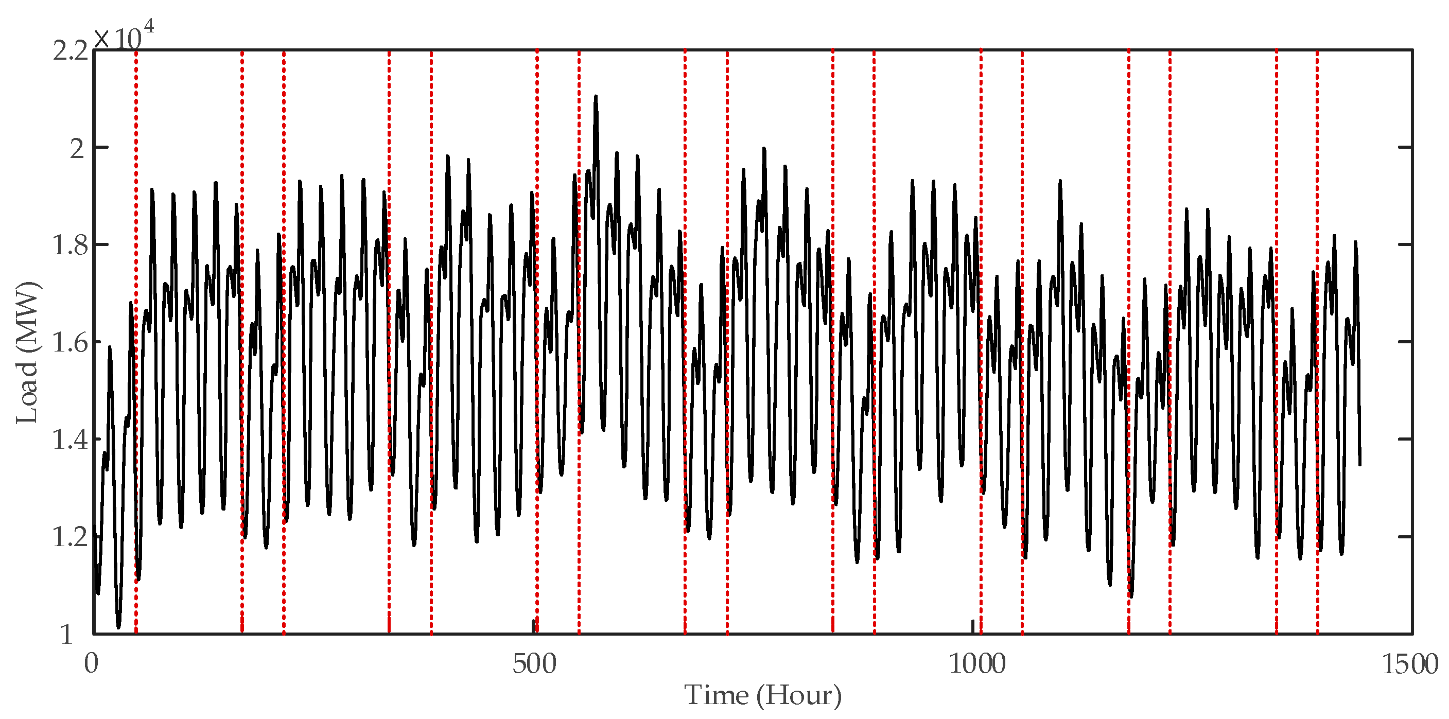
5]. The load curve from 1 January to 1 March 2011 is shown in Figure 3. The loads during working days and weekends are separated by red dashed lines [39].
(1)
Historical load. Figure 3 shows that the historical load data has the following characteristics: firstly, the load time series takes 24 h as a cycle. Secondly, the neighboring curve is similar and the load values on the different curve are close to each other at the same time. Finally, there is obvious difference between the load values during the weekends and working days. The load demands during weekends are less than working days. L(t, d) is defined as the load value at the time t ( t = 1 , 2 , , 24 ) of forecasted day. When doing day-ahead load forecasting, the load value at every hour of forecasted day is unknown. The results of the selection of historical load features are described as follows: load at time t and t − 1 of the previous day, L(t, d − 1) and L(t − 1, d − 1), load at t of the seven days before forecasted day L(t, d − 7), maximum and average load of the previous day, Lmax(d − 1) and Lmean(d − 1), load at 24 of the previous day L(24, d − 1) [40].
(2)
Day of week. Numbers from 1 to 7 represent Monday to Sunday, respectively.
(3)
Day type. Numbers 1 and 0 represent working days and weekends, respectively (the midweek holidays are identified as number 1).
(4)
Time index. The period of load time series is 24 h. Therefore, T sin ( t ) and T cos ( t ) [5] are defined as time variables to capture cycles. T sin ( t ) and T cos ( t ) can be calculated by Equations (15) and (16):
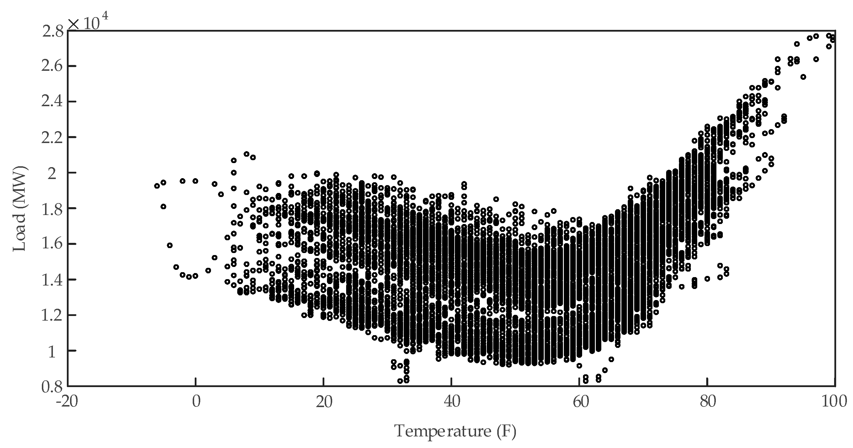
T sin ( t ) = sin ( 2 π t / 24 )
T cos ( t ) = cos ( 2 π t / 24 )
(5)
Temperature. The relationship between load and temperature in 2011 is shown in Figure 4. Figure 4 shows that load values are greatly influenced by temperature. The load values increase when the temperature is lower than 40 F or higher than 60 F. The temperature variables are selected as follows: the temperature at time t of the forecasted day T ( t ) and the previous day T(t, d − 1), the maximum and minimum temperature of the previous day, Tmax(d − 1) and Tmin(d − 1). Besides, the response time of load demand to temperature changes is larger than that of the sampling period. Therefore the average temperature of the past 3 h (Tav(3)), 6 h (Tav(6)), and 24 h (Tav(24)) are selected as temperature variables [40].
Table 1 lists the composition of the feature set.

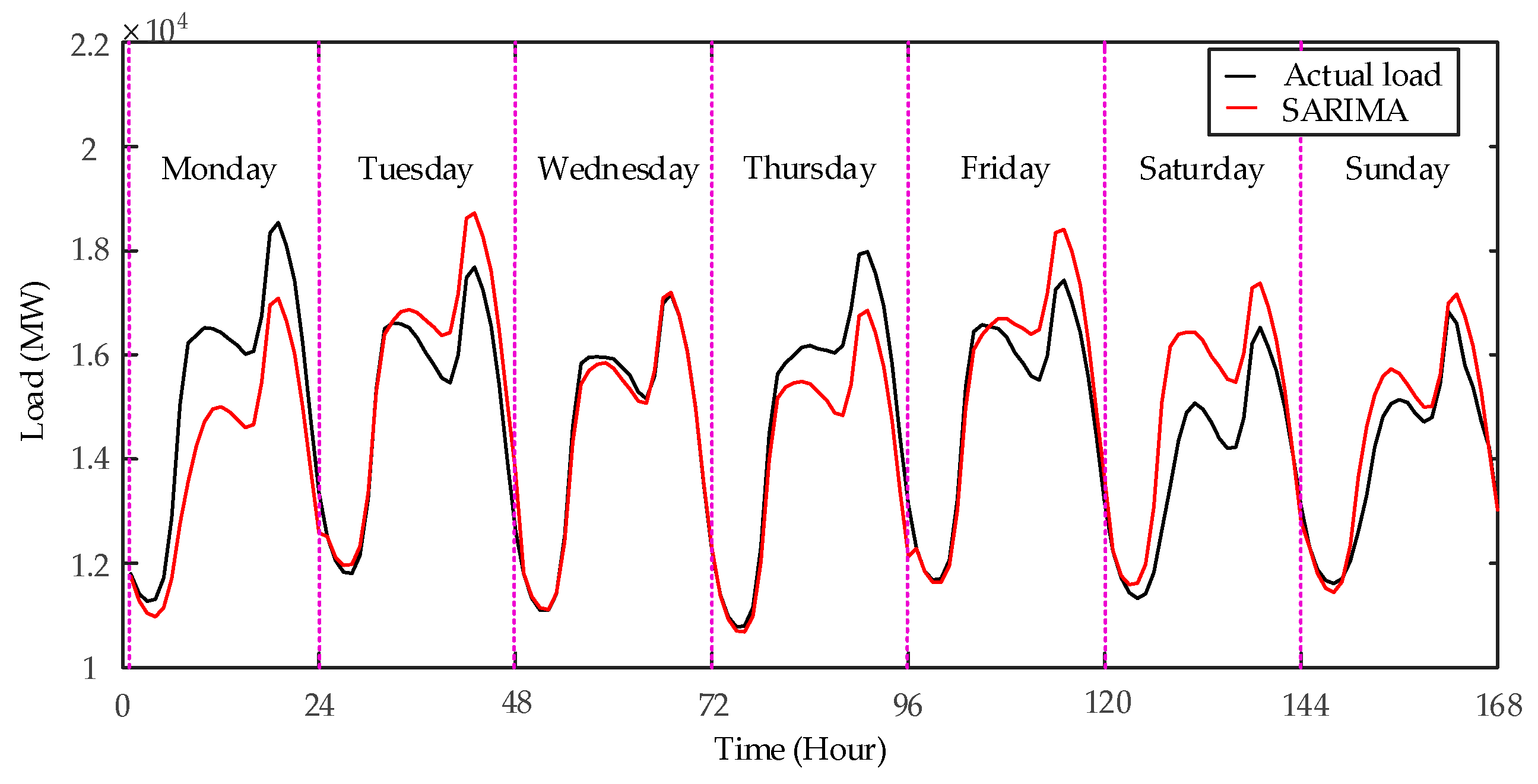
3.2. Comparison of Load Forecasting Accuracy between SARIMA and SVR

In order to analyze the influence of NWP error on the load forecasting accuracy, noisy temperature data is simulated by adding Gaussian noise to the actual temperature data. The mean value of the Gaussian noise is zero and the standard deviation is 0.6 °C [5,6]. SVR [41] and SARIMA are used to forecast the load obtained from ISO New England [5] from 6 to 12 February 2012. The mean absolute percentage error (MAPE) is adopted as criterion of error evaluation. The MAPE can be expressed as:
M A P E = 1 N t = 1 N | L ( t ) L ^ ( t ) L ( t ) | × 100 %
where L ( t ) is the actual load value, and L ^ ( t ) is the forecasting value, N is the number of samples. The results of prediction are listed in Table 2 (AT denotes the actual temperature and NT denotes a noisy temperature).
Table 2 indicates that the whole prediction accuracy of SVR is higher than that of SARIMA in working days and weekends. However, the MAPE of the SVR increases significantly when the Gaussian noise is added to the actual temperature. Without considering the impact of variables such as day types and temperature on the load, the SARIMA model is established based on the load data, so the performance of SARIMA in STLF is not good. The forecasting accuracy of SARIMA is not affected by NWP error at the same time.
From the above analysis, we can further improve the prediction efficiency of SVR by optimizing the parameters, and modify the results of SARIMA by forecasting residuals. When predicting the residuals from SARIMA, the exogenous variables such as day types and temperature will be considered.

3.3. ABC Algorithm for Parameters Selection of SVR

From the analysis in the Section 2.2, it can be known that the forecast accuracy of SVR is largely dependent on the selection of parameters including C , σ and ε. To improve the performance of SVR in STLF, the ABC algorithm is used to determine the SVR parameters in this paper. The specific steps of constructing the ABC-SVR model are as follows:
(1)
Initialize the parameters of ABC algorithm such as population of bees, maximum cycle number (MCN), abandonment cycle number (limit). The ith solution z i ( i = 1 , 2 , , F N ) of the algorithm is a vector with three elements including C, σ and ε:
z i = ( C i , σ i , ε i )
where FN is the number of solution, C, σ and ε are within the range [2−8, 28].
(2)
A worker bee finds a new solution in the neighborhood of the present solution, and calculates the fitness values of the two solutions. The fitness value is calculated by Equation (19):
f i t n e s s i = 1 1 + e i
where e i is the mean square error (MSE) of the SVR model, in which the elements of z i are chosen as SVR parameters. MSE is defined as:
e i = 1 N t = 1 N ( L ( t ) L ^ ( t ) ) 2
where L ( t ) is the actual load value, and L ^ ( t ) is the forecasting value, N is the number of samples.
(3)
The onlooker bee selects a solution by calculating the probability of the solution by Equation (14), and updates the information of the present solution.
(4)
When the number of cycles satisfies the abandonment criteria ( l i m i t ), a new solution will be generated by Equation (12).
(5)
Repeat Steps 2–4, until the number of cycles is equal to MCN.
(6)
The elements of best solution are determined as parameters of SVR.
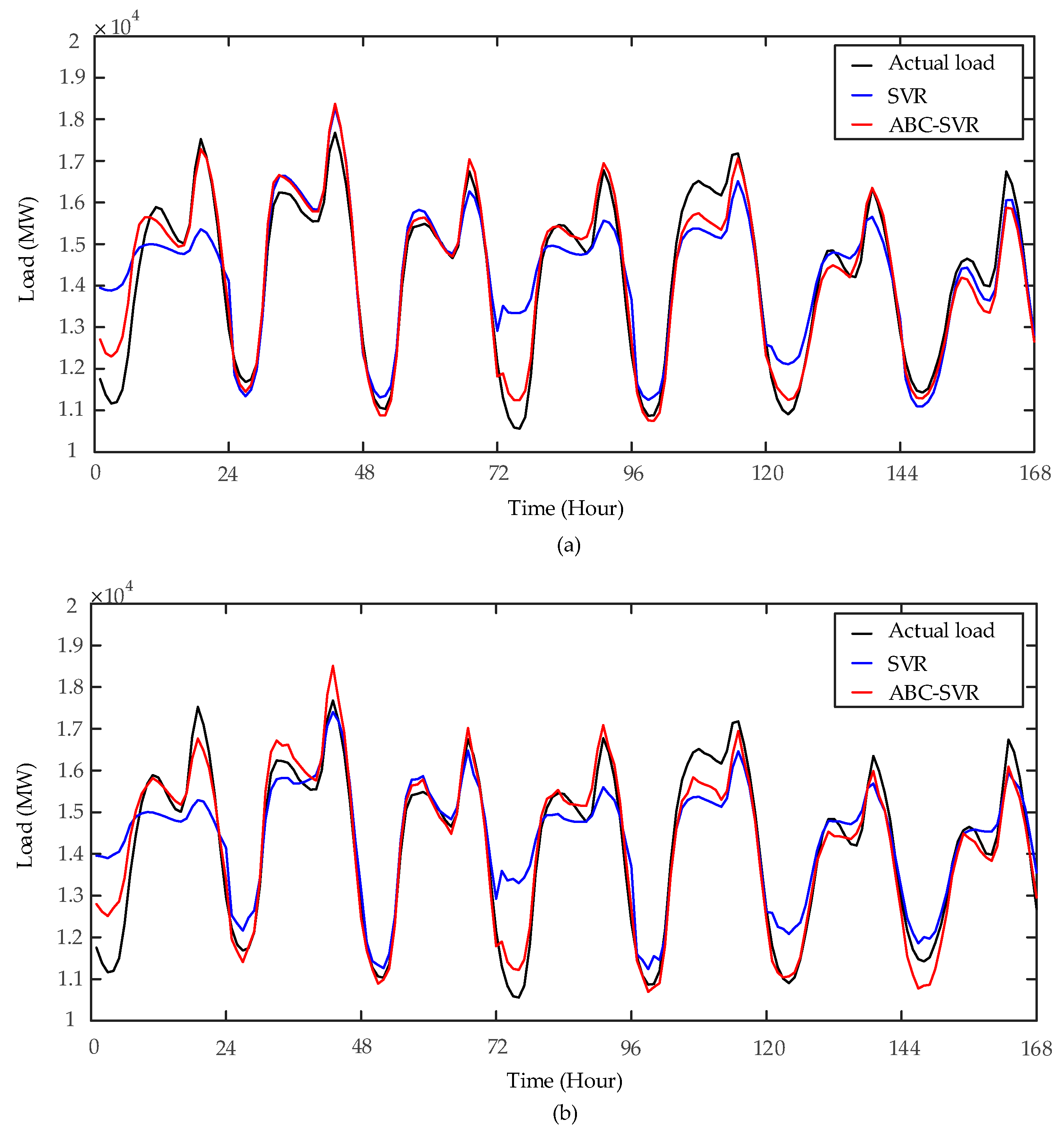
According to the above steps, the ABC-SVR model is constructed. Then, SVR and ABC-SVR are used to forecast the load from 20 to 26 February in the scenario of actual temperature and noisy temperature. The load data is obtained from ISO New England [5] and the noisy temperature is simulated by adding Gaussian noise of zero mean and standard deviation of 0.6 °C to actual temperature. The forecast results are shown in Figure 5.
Figure 5a shows that, the accuracy of SVR is obviously improved by using ABC algorithm to optimize the SVR parameters in the actual temperature scenario. The average MAPE of SVR and ABC-SVR are 4.59% and 2.43%, respectively. Figure 5b shows that the prediction accuracy of ABC-SVR is still higher than that of SVR when the noisy temperature data is used as the temperature variables of models. The average MAPE of SVR and ABC-SVR are 4.67% and 2.51%, respectively. Compared with the results achieved in scenario of actual temperature, the forecast accuracy of SVR and ABC-SVR are all decreased. The average MAPE of ABC-SVR increases from 2.52% to 2.59% during working days and increases from 2.20% to 2.31% during weekends. The increase of the forecast error in ABC-SVR is less than that in SVR. Therefore, ABC-SVR can effectively improve the prediction accuracy of SVR, but its forecast accuracy is still affected by the NWP error.

3.4. Modifying Results of SARIMA by Forecasting Residuals Using ABC-SVR

To improve the forecast accuracy of SARIMA, it is necessary to enhance the response ability of the model responses to exogenous variables. The AS-SARIMA models are constructed by using ABC-SVR to modify the results of the SARIMA. The steps of building the AS-SARIMA models are described as follows.
(1)
Establish reasonable SARIMA models for STLF, then obtain the historical residuals and load values of forecasted day from SARIMA.
(2)
Build the ABC-SVR models to forecast the residuals achieved from Step 1, then obtain the residuals of the forecasted day. The same variables including day of week, day type, time index and temperature variables as described in Section 3.1 are selected as the inputs of the model. Particularly, the historical load variables are replaced by historical residuals variables when construct the feature set of ABC-SVR.
(3)
By adding the output values of ABC-SVR to the output values of SARIMA, the final load forecasting values are obtained.
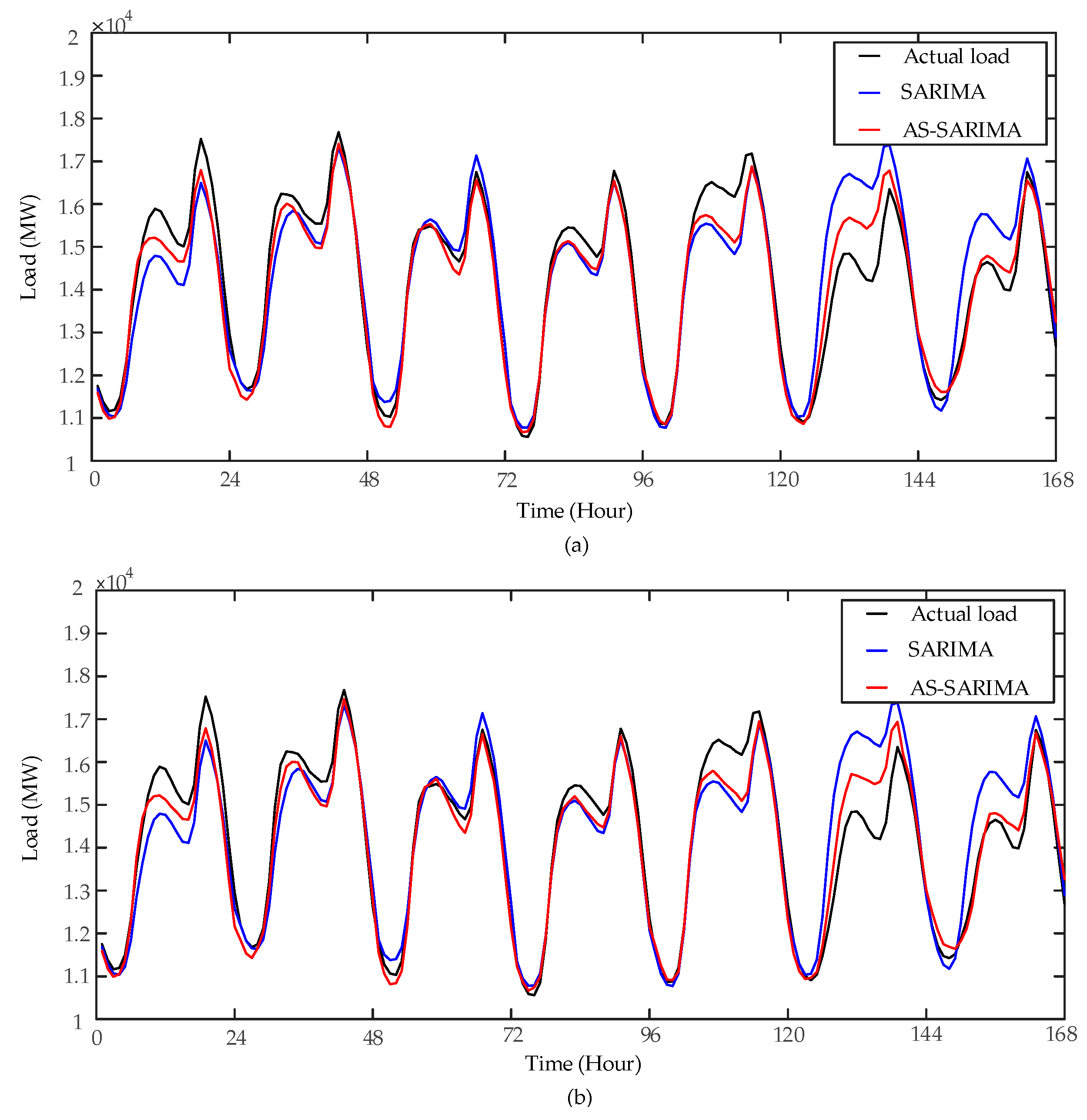
SARIMA and AS-SARIMA models are used to forecast the load from 20 to 26 February 2012 in the scenarios of actual temperature and noisy temperature. The Gaussian noise of zero mean and standard deviation of 0.6 °C is added to the measured temperature to simulated noisy temperature. The above data are achieved from ISO New England [5]. The load forecast results are shown in Figure 6. Figure 6a shows that, the forecast accuracy of AS-SARIMA is significantly higher than that of SARIMA in the scenario of actual temperature. The MAPE of SARIMA and AS-SARIMA are 4.03% and 2.34%, respectively. Figure 6b shows that by considering the temperature variables, the MAPE of AS-SARIMA increases from 2.34% to 2.36%, but the overall prediction accuracy of AS-SARIMA is still higher than that of SARIMA. Therefore, although the prediction accuracy of the AS-SARIMA is affected by the NWP error, it is still superior to the forecast accuracy of the SARIMA.

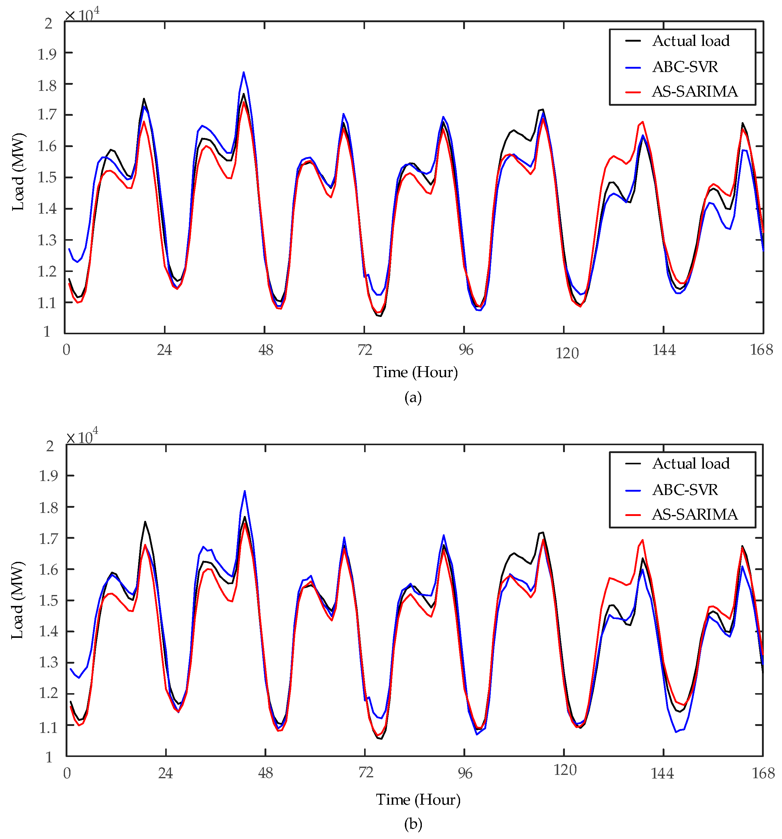
3.5. Comparison of Forecast Accuracy of ABC-SVR and AS-SARIMA and Construction of the Proposed Method

In order to compare the prediction accuracy of optimal approaches and analyze the forecasting performance affected by NWP errors of the two models, ABC-SVR and AS-SARIMA are used to forecast the load from 20 to 26 February in the scenarios of actual temperature and noisy temperature. The Gaussian noise of zero mean and standard deviation of 0.6 °C is added to actual temperature. The forecast curves of ABC-SVR and AS-SARIMA are shown in Figure 7, and the MAPE of the two models are listed in Table 3 (where AT denotes actual temperature, NT denotes noisy temperature). In Table 3, shadowed areas are results of forecasting load in working days and weekends correspondingly generated by AS-SARIMA and ABC-SVR.
Figure 7 and Table 3 show that, when forecasting the load during weekends in the scenario of actual temperature, the average MAPE generated by ABC-SVR and AS-SARIMA are 2.20% and 2.92%, respectively. With considering the NWP errors, the average of the two models are 2.31% and 3.00%. Therefore, the ABC-SVR has higher prediction accuracy than AS-SARIMA for weekend load forecasting. When forecasting the load during working days, the average MAPE of ABC-SVR and AS-SARIMA are 2.52% and 2.11% in the actual temperature scenario. After considering the NWP errors, the average MAPE of the two models are 2.59% and 2.10%. Therefore, the forecasting performance of AS-SARIMA is better than that of ABC-SVR during working days.

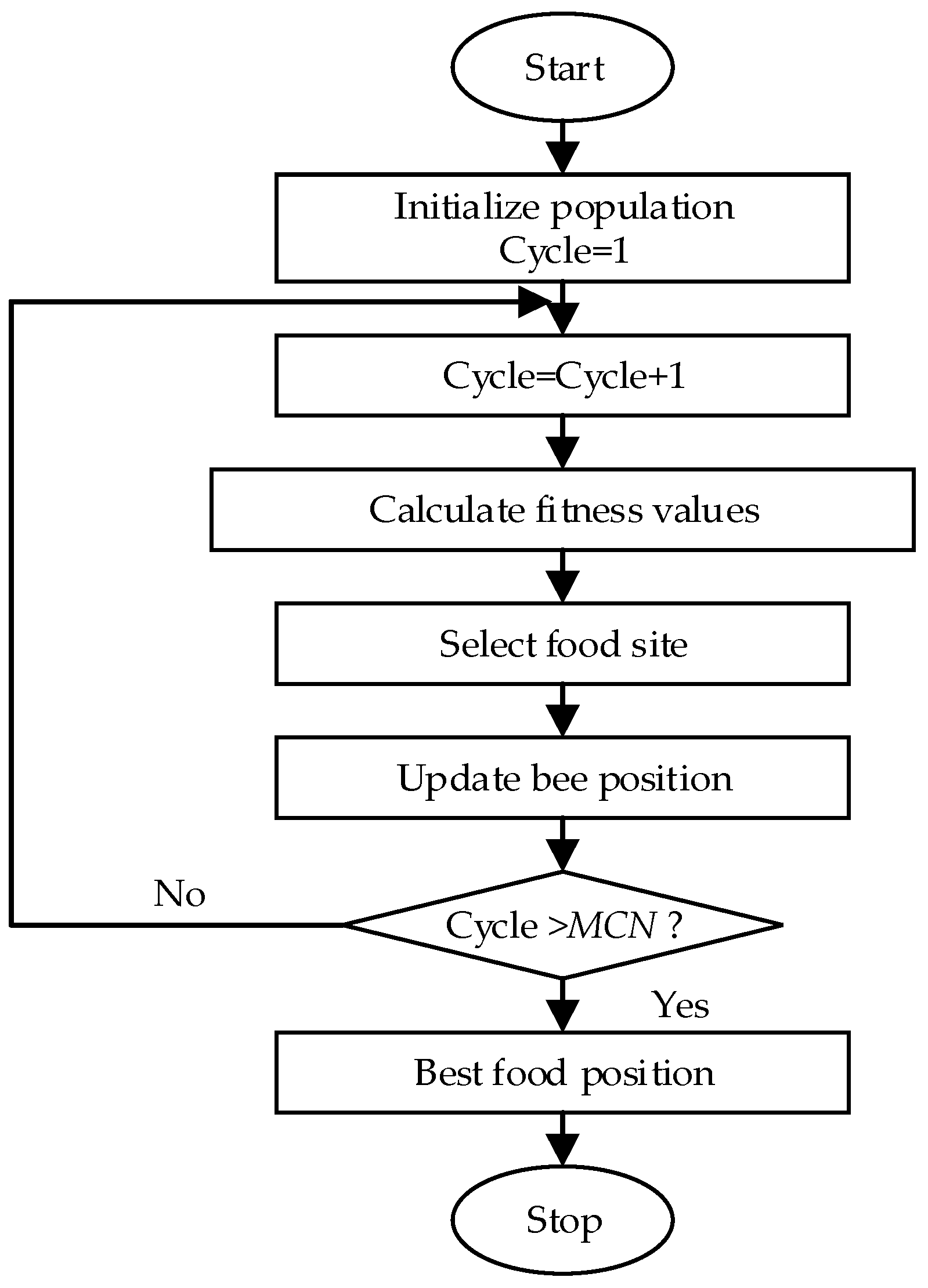
3.6. The Establishment of the Proposed Method

According to the above analysis, it is concluded that the ABC-SVR model is suitable for forecasting load in weekends and the AS-SARIMA model is suitable for forecasting the load in the working days, so a novel hybrid forecast method can be constructed by using ABC-SVR and AS-SARIMA to forecast the weekends and working days load values, respectively. The efficiency of the proposed method in the scenarios of actual temperature and noisy temperature with the Gaussian noise of standard deviations of 0.6 °C has been preliminarily proved through the above comparative experiments.
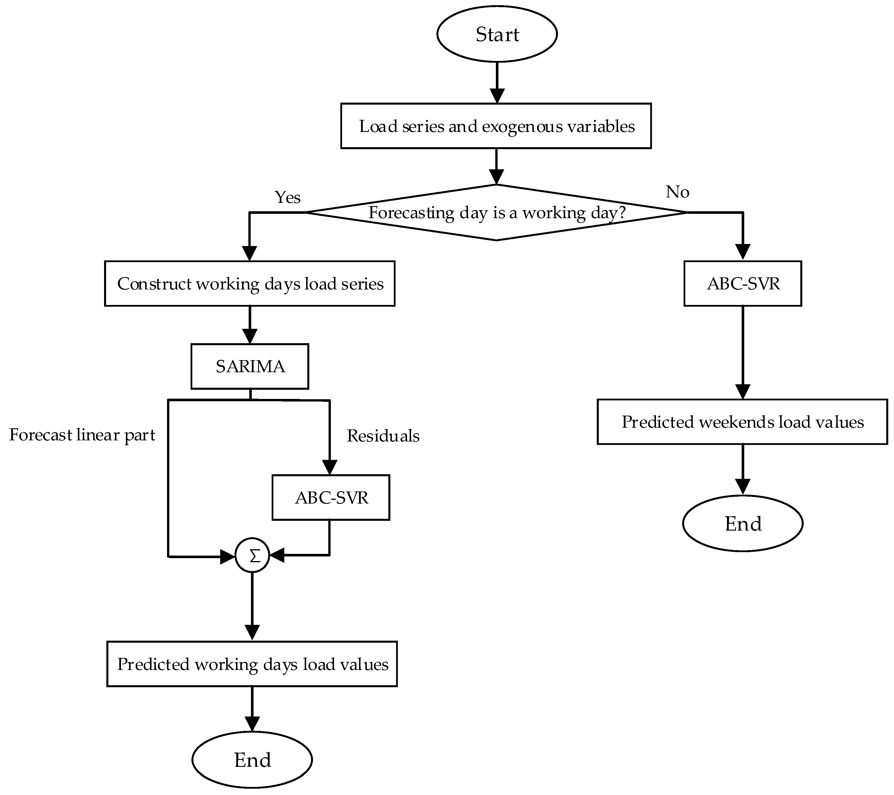
When forecasting the load in working days, the load data of first 20 working days (without weekends) are used to construct historical working days load series. By build the SARIMA models, the residuals of the first 20 working days are achieved. Then, the ABC-SVR model is established to forecast the residuals from SARIMA. Finally, the predicted load in working days is obtained by using ABC-SVR to modify the results from SARIMA. When ABC-SVR models are constructed to forecast the load during weekends, data of the first 20 days (including working days and weekends) are used as training samples. The flowchart of the proposed method is shown in Figure 8.

4. Experimental Results and Analysis

To verify the validity of proposed model, experiments using the data from 1 December 2011 to 31 December 2012 are performed.

4.1. Forecasting Results of the Proposed Method

The data of the first 20 days are selected as training samples and the load values in the next day are selected as testing samples. In order to analyze the influence of the NWP errors on prediction results, the Gaussian noise of zero mean and standard deviation of 0.6 °C is added to actual temperature to simulate the forecasting temperature data. The proposed method is used to forecast the load in four weeks of the four seasons. The experimental results are shown in Figure 9 and the MAPE of the proposed method are presented in Table 4 (where AT denotes the actual temperature and NT denotes a noisy temperature). Figure 9 and Table 4 show that the prediction accuracy of the proposed is high and less affected by the NWP errors.

4.2. Comparison and Discussion

4.2.1. Comparison of Forecast Accuracy of Different Models

In order to fully verify the effectiveness of the proposed method, ABC-SVR_WT (without considering the temperature variables, the features including load variables, day of week, day type and time index as described in Section 3.1 are selected as inputs of ABC-SVR_WT), ABC-SVR (the complete feature variables as described in Section 3.1 are selected as inputs of ABC-SVR) and AS-SARIMA are used to forecast the load in four weeks of four seasons in the scenarios of actual temperature and noisy temperature. The data from ISO New England [5] are used and the Gaussian noise of zero mean and standard deviation of 0.6 °C is added to actual temperature to simulate the noisy temperature. The MAPE of the four models are listed in Table 5, Table 6, Table 7 and Table 8 (AT denotes actual temperature, NT denotes noisy temperature).
Table 5, Table 6, Table 7 and Table 8 show that, without considering the NWP error, the average MAPE of the four weeks generated by ABC-SVR_WT, ABC-SVR, AS-SARIMA and the proposed method is 4.04%, 2.54%, 2.29% and 1.88%, respectively. The average MAPE of ABC-SVR_WT is larger than that of ABC-SVR. After adding the Gaussian noise to the actual temperature data, the MAPE of ABC-SVR_WT is still 4.04% and the corresponding MAPEs of ABC-SVR, AS-SARIMA and the proposed method are 2.59%, 2.31% and 1.90%, respectively. The error of ABC-SVR_WT is still greater than that of ABC-SVR. Therefore, it is necessary to add the temperature variables to the feature set as inputs of the models. Meanwhile, compared with ABC-SVR_WT, ABC-SVR and AS-SARIMA, the proposed method has the best performance in different scenarios.

4.2.2. Comparison of Experimental Results with Different Numerical Weather Prediction Errors

To further prove the efficiency of the proposed method with various temperature errors, the Gaussian noises of zero mean and different standard deviations are added to the actual temperature data in this case. The standard deviations of 0.6 °C, 0.9 °C and 1.2 °C are selected. The ABC-SVR, AS-SARIMA and the proposed method are used to forecast the load in the four weeks of four seasons in 2012. The data are obtained from ISO New England [5]. The experimental results are shown in Figure 10. AT denotes actual temperature, NT1, NT2 and NT3 denotes the noisy temperature with the Gaussian noise of standard deviations of 0.6 °C, 0.9 °C and 1.2 °C.
Figure 10 shows that the increases in MAPE of the three models are not large when the Gaussian noise with standard deviation of 0.6 °C. But when the standard deviations are 0.9 °C and 1.2 °C, the forecasting errors of ABC-SVR are obviously larger than those obtained in the scenario of actual temperature. Compared to ABC-SVR, the forecasting accuracy of the AS-SARIMA and the proposed method is less affected by the Gaussian noise with standard deviations of 0.9 °C and 1.2 °C. The experimental results are shown in Figure 9.
Table 9 indicates that, after adding the Gaussian noise with standard deviation of 0.6 °C to the actual temperature, the temperature error varies in the interval [−2.2 °C, 2.3 °C]. Considering the improvement of NWP accuracy, the temperature prediction error in the interval is reasonable [5]. In addition, when the standard deviations are 0.9 °C and 1.2 °C, the temperature errors vary in the intervals [−3.3 °C, 3.5 °C] and [−4.4 °C, 4.4 °C], respectively. Meanwhile, the forecast results of different models show that the prediction accuracy of the ABC-SVR is the lowest and the most affected by temperature errors at any level. When the standard deviations of Gaussian noises are 0.6 °C and 0.9 °C, the rises of MAPE generated by AS-SARIMA and the proposed method are same. When the standard deviation of the noise is 1.2 °C, the rise of MAPE generated by the proposed method is slightly greater than that generated by AS-SARIMA. However, the proposed method always has the highest forecast accuracy.

5. Conclusions

By comparing the experimental results for different models in forecasting load in various day types and analyzing the effects of temperature errors on prediction accuracy of each model, a new method based on ABC-SVR and AS-SARIMA is proposed in this paper. The advantages of the proposed method are as follows:
(1)
Through using the ABC algorithm to optimize the parameters of SVR, the ABC-SVR model is constructed. It could improve the forecast accuracy of SVR by avoiding the selection of unreasonable parameters in the model.
(2)
Considering the fluctuation of the load in weekends and comparing the prediction accuracy of different models, the ABC-SVR is used to forecast the load on weekends. When an ABC-SVR model is established, the exogenous variables such as temperature and day types are selected in addition to the historical load as the input variables of the model, so the forecast accuracy of the ABC-SVR approach is satisfactory.
(3)
Considering the stability of the working days load and the influence of the exogenous variables on load, AS-SARIMA is used to forecast the load on working days. In the AS-SARIMA model, SARIMA is used to forecast original load values and ABC-SVR is used to.
(4)
Modify the results of SARIMA by forecasting the residuals. Therefore, the prediction accuracy of the AS-SARIMA is high and little affected by NWP errors for working days load forecasting.
The simulation results based on real load data demonstrate that the proposed method has nice performance considering the NWP errors in STLF. To further improve the accuracy of STLF, more effective forecasting models and feature selection methods will be considered in future research.

Acknowledgments

This work is supported by the National High Technology Research and Development Program (863 Program) of China (No. SS2014AA052502), the Science and Technology Development Project of Jilin Province (No. 20160411003XH, No. 20160204004GX) and the Science and Technology Foundation of Department of Education of Jilin Province (2016, No. 90).

Author Contributions

Guowei Cai put forward to the main idea and design the whole venation of this paper. Wenjin Wang did the experiments and prepared the manuscript. Junhai Lu guided the experiments and paper writing.

Conflicts of Interest

The authors declare no conflict of interest.

References

  1. Raza, M.Q.; Khosravi, A. A review on artificial intelligence based load demand forecasting techniques for smart grid and buildings. Renew. Sustain. Energy Rev. 2015, 50, 1352–1372. [Google Scholar] [CrossRef]
  2. Bozic, M.; Stojanovic, M.; Stajic, Z.; Floranovic, N. Mutual information-based inputs selection for electric load time series forecasting. Entropy 2013, 15, 926–942. [Google Scholar] [CrossRef]
  3. Kouhi, S.; Keynia, F. A new cascade NN based method to short-term load forecast in deregulated electricity market. Energy Convers. Manag. 2013, 71, 76–83. [Google Scholar] [CrossRef]
  4. Kulkarni, S.; Simon, S.P.; Sundareswaran, K. A spiking neural network (SNN) forecast engine for short-term electrical load forecasting. Appl. Soft Comput. 2013, 13, 3628–3635. [Google Scholar] [CrossRef]
  5. Li, S.; Wang, P.; Goel, L. Short-term load forecasting by wavelet transform and evolutionary extreme learning machine. Electr. Power Syst. Res. 2015, 122, 96–103. [Google Scholar] [CrossRef]
  6. Reis, A.J.R.; da Silva, A.P.A. Feature extraction via multiresolution analysis for short-term load forecasting. IEEE Trans. Power Syst. 2005, 20, 189–198. [Google Scholar]
  7. Sudheer, G.; Suseelatha, A. Short term load forecasting using wavelet transform combined with Holt–Winters and weighted nearest neighbor models. Int. J. Electr. Power 2015, 64, 340–346. [Google Scholar] [CrossRef]
  8. Wang, J.J.; Wang, J.Z.; Li, Y.N.; Zhu, S.L.; Zhao, J. Techniques of applying wavelet de-noising into a combined model for short-term load forecasting. Int. J. Electr. Power 2014, 62, 816–824. [Google Scholar] [CrossRef]
  9. Li, S.; Wang, P.; Goel, L. A novel wavelet-based ensemble method for short-term load forecasting with hybrid neural networks and feature selection. IEEE Trans. Power Syst. 2016, 31, 1788–1798. [Google Scholar] [CrossRef]
  10. Gu, C.J.; Yang, D.Z.; Jirutitijaroen, P.; Walsh, W.M.; Reindl, T. Spatial load forecasting with communication failure using time-forward kriging. IEEE Trans. Power Syst. 2014, 29, 2875–2882. [Google Scholar]
  11. Lee, W.J.; Hong, J. A hybrid dynamic and fuzzy time series model for mid-term power load forecasting. Int. J. Electr. Power 2015, 64, 1057–1062. [Google Scholar] [CrossRef]
  12. Niu, D.X.; Shi, H.F.; Wu, D.D. Short-term load forecasting using bayesian neural networks learned by Hybrid Monte Carlo algorithm. Appl. Soft Comput. 2012, 12, 1822–1827. [Google Scholar] [CrossRef]
  13. Hooshmand, R.A.; Amooshahi, H.; Parastegari, M. A hybrid intelligent algorithm based short-term load forecasting approach. Int. J. Electr. Power 2013, 45, 313–324. [Google Scholar] [CrossRef]
  14. Chaturvedi, D.K.; Sinha, A.P.; Malik, O.P. Short term load forecast using fuzzy logic and wavelet transform integrated generalized neural network. Int. J. Electr. Power 2015, 67, 230–237. [Google Scholar] [CrossRef]
  15. Kouhi, S.; Keynia, F.; Ravadanegh, S.N. A new short-term load forecast method based on neuro-evolutionary algorithm and chaotic feature selection. Int. J. Electr. Power 2014, 62, 862–867. [Google Scholar] [CrossRef]
  16. Ko, C.N.; Lee, C.M. Short-term load forecasting using SVR (support vector regression)-based radial basis function neural network with dual extended Kalman filter. Energy 2013, 49, 413–422. [Google Scholar] [CrossRef]
  17. Ceperic, E.; Ceperic, V.; Baric, A. A strategy for short-term load forecasting by support vector regression machines. IEEE Trans. Power Syst. 2013, 28, 4356–4364. [Google Scholar] [CrossRef]
  18. Kavousi-Fard, A.; Samet, H.; Marzbani, F. A new hybrid modified firefly algorithm and support vector regression model for accurate short term load forecasting. Expert Syst. Appl. 2014, 41, 6047–6056. [Google Scholar] [CrossRef]
  19. Che, J.X.; Wang, J.Z. Short-term load forecasting using a kernel-based support vector regression combination model. Appl. Energy 2014, 132, 602–609. [Google Scholar] [CrossRef]
  20. Hu, Z.Y.; Bao, Y.K.; Xiong, T. Comprehensive learning particle swarm optimization based memetic algorithm for model selection in short-term load forecasting using support vector regression. Appl. Soft Comput. 2014, 25, 15–25. [Google Scholar] [CrossRef]
  21. Lin, C.T.; Chou, L.D.; Chen, Y.M.; Tseng, L.M. A hybrid economic indices based short-term load forecasting system. Int. J. Electr. Power 2014, 54, 293–305. [Google Scholar] [CrossRef]
  22. Moazzami, M.; Khodabakhshian, A.; Hooshmand, R. A new hybrid day-ahead peak load forecasting method for Iran’s National Grid. Appl. Energy 2013, 101, 489–501. [Google Scholar] [CrossRef]
  23. Wang, J.J.; Li, L.; Niu, D.X.; Tan, Z.F. An annual load forecasting model based on support vector regression with differential evolution algorithm. Appl. Energy 2012, 94, 65–70. [Google Scholar] [CrossRef]
  24. Quan, H.; Srinivasan, D.; Khosravi, A. Uncertainty handling using neural network-based prediction intervals for electrical load forecasting. Energy 2014, 73, 916–925. [Google Scholar] [CrossRef]
  25. Che, J.X. A novel hybrid model for bi-objective short-term electric load forecasting. Int. J. Electr. Power 2014, 61, 259–266. [Google Scholar] [CrossRef]
  26. Hong, W.C.; Dong, Y.C.; Zhang, W.Y.; Chen, L.Y.; Panigrahi, B.K. Cyclic electric load forecasting by seasonal SVR with chaotic genetic algorithm. Int. J. Electr. Power 2013, 44, 604–614. [Google Scholar] [CrossRef]
  27. Chen, Y.H.; Yang, Y.; Liu, C.Q.; Li, C.H.; Li, L. A hybrid application algorithm based on the support vector machine and artificial intelligence: An example of electric load forecasting. Appl. Math. Model. 2015, 39, 2617–2632. [Google Scholar] [CrossRef]
  28. Yan, X.; Chowdhury, N.A. Mid-term electricity market clearing price forecasting utilizing hybrid support vector machine and auto-regressive moving average with external input. Int. J. Electr. Power 2014, 63, 64–70. [Google Scholar] [CrossRef]
  29. Zhang, W.Y.; Hong, W.C.; Dong, Y.C.; Tsai, G.; Sung, J.T.; Fan, G.F. Application of SVR with chaotic GASA algorithm in cyclic electric load forecasting. Energy 2012, 45, 850–858. [Google Scholar] [CrossRef]
  30. Hong, W.C. Chaotic particle swarm optimization algorithm in a support vector regression electric load forecasting model. Energy Convers. Manag. 2009, 50, 105–117. [Google Scholar] [CrossRef]
  31. Yang, D.; Liu, Y.; Li, S.; Li, X.; Ma, L. Gear fault diagnosis based on support vector machine optimized by artificial bee colony algorithm. Mech. Mach. Theory 2015, 90, 219–229. [Google Scholar] [CrossRef]
  32. Mandal, S.K.; Chan, F.T.S.; Tiwari, M.K. Leak detection of pipeline: An integrated approach of rough set theory and artificial bee colony trained SVM. Expert Syst. Appl. 2012, 39, 3071–3080. [Google Scholar] [CrossRef]
  33. Kang, F.; Li, J. Artificial bee colony algorithm optimized support vector regression for system reliability analysis of slopes. J. Comput. Civ. Eng. 2015, 30. [Google Scholar] [CrossRef]
  34. Karaboga, D.; Ozturk, C.; Karaboga, N.; Gorkemli, B. Artificial bee colony programming for symbolic regression. Inf. Sci. 2012, 209, 1–15. [Google Scholar] [CrossRef]
  35. Mernik, M.; Liu, S.H.; Karaboga, D.; Crepinsek, M. On clarifying misconceptions when comparing variants of the Artificial Bee Colony Algorithm by offering a new implementation. Inf. Sci. 2015, 291, 115–127. [Google Scholar] [CrossRef]
  36. El-Fergany, A.A.; Abdelaziz, A.Y. Capacitor placement for net saving maximization and system stability enhancement in distribution networks using artificial bee colony-based approach. Int. J. Electr. Power 2014, 54, 235–243. [Google Scholar] [CrossRef]
  37. Karaboga, D.; Gorkemli, B.; Ozturk, C.; Karaboga, N. A comprehensive survey: Artificial bee colony (ABC) algorithm and applications. Artif. Intell. Rev. 2014, 42, 21–57. [Google Scholar] [CrossRef]
  38. Areekul, P.; Senjyu, T.; Toyama, H.; Yona, A. Notice of violation of IEEE publication principles a hybrid ARIMA and neural network model for short-term price forecasting in deregulated market. IEEE Trans. Power Syst. 2010, 25, 524–530. [Google Scholar] [CrossRef]
  39. Hu, Z.Y.; Bao, Y.K.; Xiong, T.; Chiong, R. Hybrid filter-wrapper feature selection for short-term load forecasting. Eng. Appl. Artif. Intell. 2015, 40, 17–27. [Google Scholar] [CrossRef]
  40. Ding, N.; Benoit, C.; Foggia, G.; Besanger, Y.; Wurtz, F. Neural network-based model design for short-term load forecast in distribution systems. IEEE Trans. Power Syst. 2016, 31, 72–81. [Google Scholar] [CrossRef]
  41. Che, J.X.; Wang, J.Z.; Tang, Y.J. Optimal training subset in a support vector regression electric load forecasting model. Appl. Soft Comput. 2012, 12, 1523–1531. [Google Scholar] [CrossRef]
Figure 1. Curves of original load and load predicted by seasonal autoregressive integrated moving average (SARIMA).
Energies 09 00994 g001
Figure 2. The flowchart of the artificial bee colony (ABC) algorithm. MCN: maximum cycle number.
Energies 09 00994 g002
Figure 3. Load from 1 January to 1 March 2011.
Energies 09 00994 g003
Figure 4. Relationship between load and temperature.
Energies 09 00994 g004
Figure 5. Load curves predicted by SVR and ABC-SVR. (a) Actual temperature; and (b) noisy temperature.
Energies 09 00994 g005
Figure 6. Load curves predicted by SARIMA and AS-SARIMA. (a) Actual temperature; and (b) noisy temperature.
Energies 09 00994 g006
Figure 7. Load curves predicted by ABC-SVR and AS-SARIMA. (a) Actual temperature; and (b) noisy temperature.
Energies 09 00994 g007
Figure 8. The flowchart of the proposed method.
Energies 09 00994 g008
Figure 9. Load curves predicted by the proposed method in 2012. (a) Prediction result from 22 to 28 February; (b) prediction result from 18 to 24 May; (c) prediction result from 8 to 14 August; and (d) prediction result from 15 to 21 November.
Energies 09 00994 g009
Figure 10. The average MAPE of different methods in 2012. (a) Prediction from 22 to 28 February; (b) prediction from 18 to 24 May; (c) prediction from 8 to 14 August; and (d) prediction from 15 to 21 November.
Energies 09 00994 g010
Table 1. The feature set.
Type NumberVariablesFeatures
1Historical loadL(t, d − 1), L(t − 1, d − 1), L(t, d − 7), Lmax(d − 1), Lmean(d − 1), L(24, d − 1)
2Day of weekNumbers from 1 to 7
3Day type1 (working days), 0 (weekends)
4Time indexTsin(t), Tcos(t)
5TemperatureT(t), T(t, d − 1), Tmax(d − 1), Tmin(d − 1), Tav(3), Tav(6), Tav(24)
Table 2. Mean absolute percentage error (MAPE) (%) of support vector regression (SVR) and SARIMA.
DaySARIMASVR
ATNTATNT
Monday5.745.743.133.17
Tuesday0.980.981.351.44
Wednesday2.842.842.132.13
Thursday2.122.122.512.54
Friday2.112.112.372.41
Saturday4.504.502.822.75
Sunday2.812.815.235.34
Average MAPE3.013.012.792.83
Table 3. MAPE (%) of ABC-SVR and AS-SARIMA.
DayABC-SVRAS-SARIMA
ATNTATNT
Monday4.144.223.053.04
Tuesday2.072.122.052.01
Wednesday0.971.031.141.13
Thursday2.622.681.561.57
Friday2.792.902.752.76
Saturday1.581.704.094.15
Sunday2.822.921.751.84
Average MAPE2.432.512.342.36
Table 4. MAPE (%) of the proposed method.
DayWinter 22–28 FebruarySpring 18–24 May
ATNTATNT
Monday2.132.171.161.12
Tuesday1.351.350.750.77
Wednesday0.780.791.481.51
Thursday1.171.192.802.84
Friday2.732.761.141.14
Saturday1.581.701.551.64
Sunday2.822.921.801.84
Average MAPE1.791.841.531.55
DaySummer 8–14 AugustFall 15–21 November
ATNTATNT
Monday3.113.241.331.36
Tuesday2.542.891.531.53
Wednesday1.081.121.601.60
Thursday1.131.190.730.76
Friday3.523.290.620.63
Saturday3.543.341.891.99
Sunday2.682.424.084.07
Average MAPE2.512.501.681.70
Table 5. Comparison of MAPE (%) from 22 to 28 February 2012.
DayABC-SVR_WTABC-SVRAS-SARIMAProposed Method
ATNTATNTATNTATNT
22 February5.255.250.971.031.141.130.780.79
23 February2.592.592.622.681.561.571.171.19
24 February4.604.602.792.902.752.762.732.76
25 February5.345.341.581.704.094.151.581.70
26 February4.784.782.822.921.751.842.822.92
27 February6.076.075.465.522.922.882.132.17
28 February3.413.412.102.151.911.911.351.35
Average MAPE4.584.582.622.702.302.321.791.84
Table 6. Comparison of MAPE (%) from 18 to 24 May 2012.
DayABC-SVR_WTABC-SVRAS-SARIMAProposed Method
ATNTATNTATNTATNT
18 May2.952.952.052.091.271.311.141.14
19 May1.991.991.551.641.921.991.551.64
20 May2.562.561.801.841.971.991.801.84
21 May2.402.401.671.721.211.221.161.12
22 May5.995.991.411.461.311.290.750.77
23 May2.822.821.952.011.691.701.481.51
24 May3.893.893.663.772.852.882.802.84
Average MAPE3.233.232.012.081.751.771.531.55
Table 7. Comparison of MAPE (%) from 8 to 14 August 2012.
DayABC-SVR_WTABC-SVRAS-SARIMAProposed Method
ATNTATNTATNTATNT
8 August5.155.152.392.441.491.521.081.12
9 August6.506.501.481.521.301.371.131.19
10 August4.824.824.044.114.904.913.523.29
11 August4.034.033.543.343.633.623.543.34
12 August3.393.392.682.422.812.542.682.42
13 August3.363.362.892.912.692.663.113.24
14 August3.833.832.983.401.962.292.542.89
Average MAPE4.444.442.862.882.682.702.512.50
Table 8. Comparison of MAPE (%) from 15 to 21 November 2012.
DayABC-SVR_WTABC-SVRAS-SARIMAProposed Method
ATNTATNTATNTATNT
15 November4.394.392.822.861.341.370.730.76
16 November2.002.001.521.540.930.940.620.63
17 November2.492.491.891.994.814.891.891.99
18 November5.885.884.084.072.272.264.084.07
19 November5.245.244.784.814.744.731.331.36
20 November5.415.411.901.981.601.611.531.53
21 November1.851.851.581.661.421.411.601.59
Average MAPE3.893.892.652.702.442.461.681.70
Table 9. The MAPE (%) for different models with Gaussian noises of zero mean.
Standard Deviation (°C)Error Range of Temperature (°C)Models
ABC-SVRAS-SARIMAProposed Method
0n.a.2.542.291.88
0.6[−2.2, 2.3]2.592.311.90
0.9[−3.3, 3.5]2.722.381.97
1.2[−4.4, 4.4]2.842.452.07

