Wind Speed Prediction Using a Univariate ARIMA Model and a Multivariate NARX Model

Abstract

Two on step ahead wind speed forecasting models were compared. A univariate model was developed using a linear autoregressive integrated moving average (ARIMA). This method’s performance is well studied for a large number of prediction problems. The other is a multivariate model developed using a nonlinear autoregressive exogenous artificial neural network (NARX). This uses the variables: barometric pressure, air temperature, wind direction and solar radiation or relative humidity, as well as delayed wind speed. Both models were developed from two databases from two sites: an hourly average measurements database from La Mata, Oaxaca, Mexico, and a ten minute average measurements database from Metepec, Hidalgo, Mexico. The main objective was to compare the impact of the various meteorological variables on the performance of the multivariate model of wind speed prediction with respect to the high performance univariate linear model. The NARX model gave better results with improvements on the ARIMA model of between $5.5\%$ and $10.6\%$ for the hourly database and of between $2.3\%$ and $12.8\%$ for the ten minute database for mean absolute error and mean squared error, respectively.

1. Introduction

At the end of 2014, the worldwide installed wind energy generating capacity was 369,597 MW; Europe having 134,007 MW, of which Germany and Spain stood out with 39,165 and 22,987 MW, respectively. During 2015, $42\%$ of electric power in Denmark was generated from wind [1]. In the Asia-Pacific region, China had a reported capacity of 114,609 MW of a total of 141,964 MW. In North America, the reported U.S. installed capacity was 65,879 MW with the Mexican and Canadian installed capacities being 9694 and 2551 MW, respectively. In Latin America, Brazil was the leader, with 5939 MW of 8526 MW total [2].

Onshore wind based power generation has reached the technological maturity of being competitive with the lowest cost power generation options in many places. For example in Mexico in 2012 installed capacity increased by $76\%$ with respect to the total installed wind energy generation capacity at the end of 2011 due to increasing exploitation of the intense resource in the state of Oaxaca.

In Oaxaca in the corridor from La Venta to La Mata passing through La Ventosa, the annual average wind speed is over 9 m/s at 30 m above ground level with a dominant wind direction of North-Northwest/North-Northeast 70% of the time [3]. These highly favorable intense wind conditions in Oaxaca represent an appreciable source of inexpensive renewable energy in addition to Mexico’s large fossil fuel reserves, which makes its exploitation a priority.

In Mexico, the National Center for Energy Control (CENACE) is responsible for the dispatch control of energy for the National Electric System. CENACE uses an information system to prepare pre-dispatch strategies. This system takes into account: availability, derating, restrictions and other factors that affect the dispatch capacity of generating units, as well as the electricity demand forecast. These models are produced by CENACE. An hourly operation plan is essential for each unit [4]. Energy producers have a responsibility to provide forecasts of wind and net energy production to CENACE a day ahead.

Recently, a considerable number of wind speed prediction models have been developed using a range of methods, some simple and others combining various techniques. Cadenas and Rivera [5] have reported short-term wind speed forecasting in a region of Oaxaca using an artificial neural network (ANN) with a representative hourly time series for the site. The model showed good accuracy for energy supply prediction.

Salcedo-Sanz et al. [6] presented a hybrid model between a fifth generation mesoscale model (MM5) and a neural network for short-term wind speed prediction at specific points.

Cadenas et al. [7] analyzed and forecasted wind velocity in Chetumal, Quintana Roo, Mexico, with a single exponential smoothing method. The method was found to be good for wind forecasting when the field data had alpha values close to one.

Li and Shi [8] compared three artificial neural networks for wind speed forecasting. These were: adaptive linear element, back propagation and radial basis function. None of these outperformed the others on all of the metrics evaluated.

A new short-term hybrid method based on wavelet and classical time series analysis to predict wind speed and power was proposed by Liu et al. [9]. The mean relative error in multi-step forecasting using this method was smaller than that from classical time series and back-propagation network methods.

A wind speed forecasting model for three regions of Mexico was developed using a hybrid autoregressive integrated moving average technique (ARIMA-ANN) by Cadenas and Rivera [10]. Initially, the ARIMA models were used to generate wind speed forecasts for the time series. The resulting errors were used to build the ANN to account for the non-linear behavior that the ARIMA technique could not model. This reduced the errors. The results showed that the hybrid model produced higher accuracy wind speed predictions than those of the separate ARIMA and ANN models for all three sites.

Kavasseri and Seetharaman [11] used the fractional-ARIMA models to predict wind speed and power production one or two days ahead for North Dakota. Forecasting errors in wind speed and power were compared to the persistence model. Significant improvements were obtained.

Li et al. [12] presented a robust two-step method for accurate wind speed forecasting based on a Bayesian combination algorithm and three neural network models: an adaptive linear element network (ADALINE), back propagation (BP) and a radial basis function (RBF). The results were that the neural networks were not consistent for one hour ahead wind speed. However, the Bayesian combination method could always give adaptive, reliable and comparatively accurate forecasts.

Liu et al. [13] evaluated the effectiveness of autoregressive moving average-generalized autoregressive conditional heteroscedasticity (ARMA-GARCH) for modeling mean wind speed and its volatility. The results showed that ARMA-GARCH could capture the trend changes of these parameters. In this study, it was found that none of the models were consistently better than the others over the whole range of heights considered. The authors recommended that for a given dataset, all of the models should be evaluated to find the most appropriate (Given that the range of heights considered was from 10 to 80 m and that the swept diameter of wind turbines is of the order of 90 m centered at a height of 70 m for 3-MW units, the heights covered by the study needed to be greater).

Guo et al. [14] developed an empirical mode decomposition (EMD) based feed-forward neural network (FFNN) learning model, which resulted in improved accuracy over each of the two methods individually for predicting daily and monthly mean wind speeds.

Liu et al. [15] have proposed hybrid ARIMA-ANN and ARIMA-Kalman methods for hourly wind speed forecasting. The authors concluded that both methods gave good results and can be applied to dynamic wind speed forecasting for wind power systems.

Kalman filtering was optimized for application to very short-term wind forecasting and applied to wind energy for a site at Varese Ligure in Italy by Cassola and Burlando [16]. A numerical meteorological model BOLAM (Bologna Limited Area Model) was used, and the results with the application of Kalman filtering showed a considerable reduction in error.

On the basis of parameter selection and data decomposition, two combined strategies and four modified models based on the first-order and second-order adaptive coefficient (FAC and SAC) were proposed by Zhang et al. [17] for wind speed forecasting in four different sites in China. It was shown that the approaches derived from the combined strategies obtained higher prediction accuracy than the individual FAC and SAC models at the four sampled sites.

A hybrid model based on the EMD and ANNs named EMD-ANN for wind speed prediction was proposed by Liu et al. [18]. The results were compared to an ANN model and an autoregressive integrated moving average model. These showed that the performance of the model was very good compared to the individual methods.

Two prediction methods were studied by Peng et al. [19] for short-term wind power forecasting on a wind farm. Three key factors were used in the models: temperature, wind speed and direction. One was an artificial neural network and the other a hybrid model based on physical and statistical methods. The hybrid model produced higher accuracy results than the individual ANN model.

Chen and Yu [20] developed a hybrid model that integrated a support vector regression (SVR)-based state-space model with an unscented Kalman filter (UKF). This was to predict short-term wind speed sequences. The results gave much better performance for both one step and multi-step ahead wind speed forecasts than support vector machine, autoregressive and ANNs.

Hocaoglu et al. [21] developed a model for the artificial prediction of wind speed data, from atmospheric pressure measurements using the hidden Markov models (HMMs) technique. The model accuracy was evaluated from Weibull distribution parameters. The relevance of the technique is in its use of an additional meteorological variable (atmospheric pressure).

Hocaoglu et al. [22] used the Mycielski algorithm for wind speed forecasting. The algorithm performs a prediction using the total exact history of the data samples. The basic idea of the algorithm was to search for the longest suffix string at the end of the data sequence that had been repeated at least once in the history of the sequence. It was concluded that the model was robust for different behaviors of wind speed patterns. Experimental results also showed that the model not only provided very consistent time variations in agreement with the actual measured data, but also provides accurate distribution model parameters for estimating the wind power potential of a region.

Of all of the models reviewed, only two use additional meteorological parameters other than wind speed, such as pressure and temperature.

In this work, wind speed forecasting for La Mata, Oaxaca, and Metepec, Hidalgo, was carried out using univariate and multivariate models. To achieve higher accuracy forecasts, wind speed models using non-linear auto-regressive exogenous (NARX) modeling were developed. This technique uses additional exogenous variables (i.e., other than wind speed) to generate more accurate forecasts with respect to ARIMA models solely based on wind speed time series. The meteorological variables used in this study were: wind speed and direction, solar radiation, temperature and pressure. In the generation of the NARX model, only solar radiation or relative humidity was used due to the results from a correlation study.

2. Experimental Data

Two weather databases were used as sources of information to allow the wind speed prediction models to be tested under a range of conditions. The time series of the variables used in this analysis are shown in Figure 1, Figure 2, Figure 3, Figure 4, Figure 5 and Figure 6.

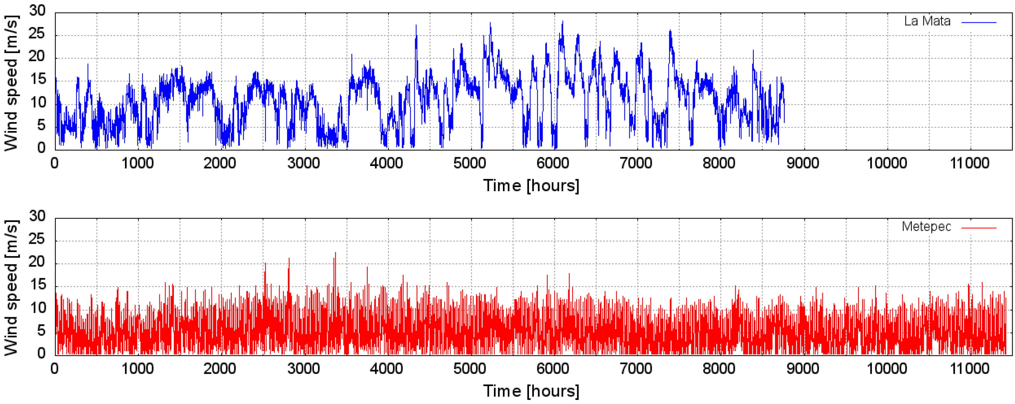
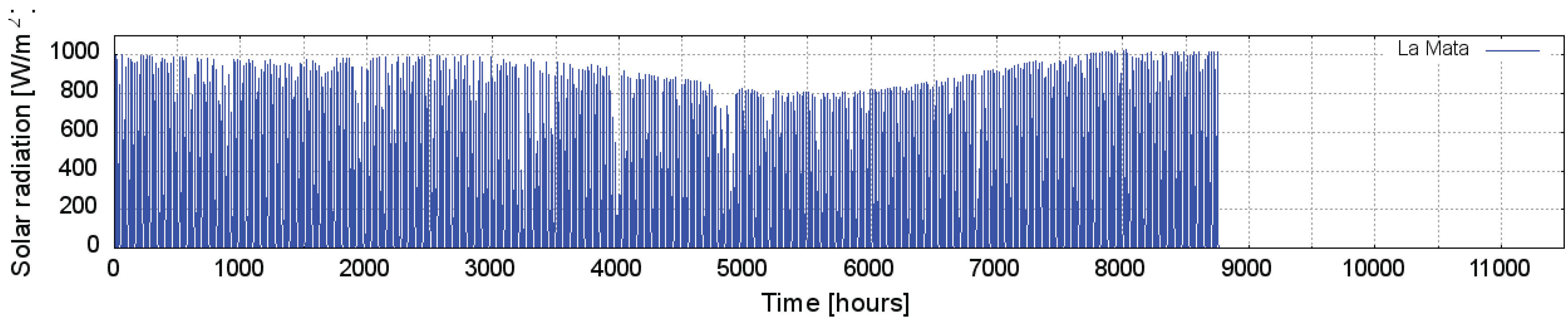
One data set was from observations in the town of La Mata in the state of Oaxaca, Mexico. This was provided by the Mexican Federal Electricity Commission (Comision Federal de Electricidad (CFE)) and has 8759 data points corresponding to one year of hourly averaged measurements taken at 40 m above ground level from 1 May 2006 to 30 April 2007. The measurements were: wind speed, WS (m/s); wind direction, WD (${}^{\circ }$); barometric pressure, P (mbar), air temperature, T (${}^{\circ }$C), and solar radiation, SR (W/m${}^2$).

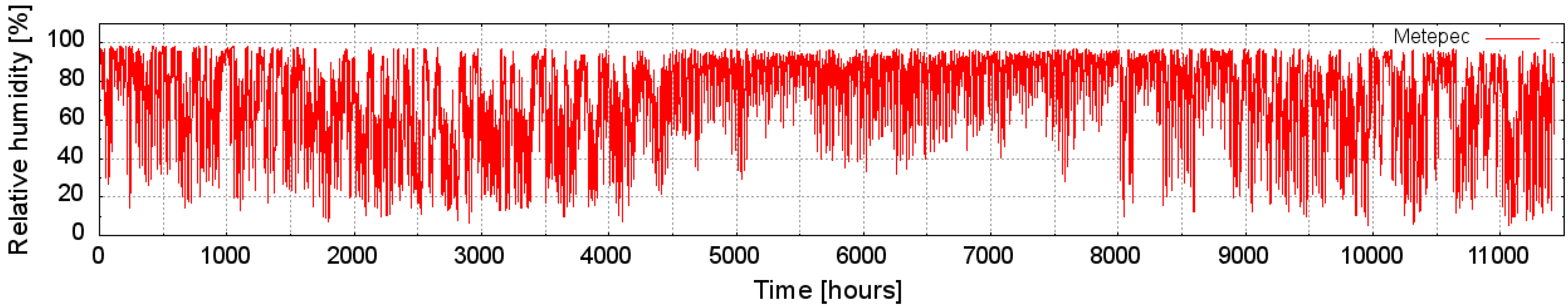
The other data set was from observations in the town of Metepec in the state of Hidalgo, Mexico. This was provided also by the CFE and has 68,550 data points which correspond to just over a year and three months of ten minutely averaged measurements. The measurements were made at a height of 50 m above ground level from 22 November 2007 to 12 March 2009. The measurements were: wind speed, WS (m/s); wind direction, WD (${}^{\circ }$); barometric pressure, P (mbar), air temperature, T (${}^{\circ }$C), and relative humidity, RH (%).

Figure 1 shows the measured wind speed for both stations. It can be appreciated that there are no tendencies for neither periodic nor seasonal wind speed variations in the time series. The average wind speeds are 10.9 and 5.2 m/s for La Mata and Metepec, respectively.

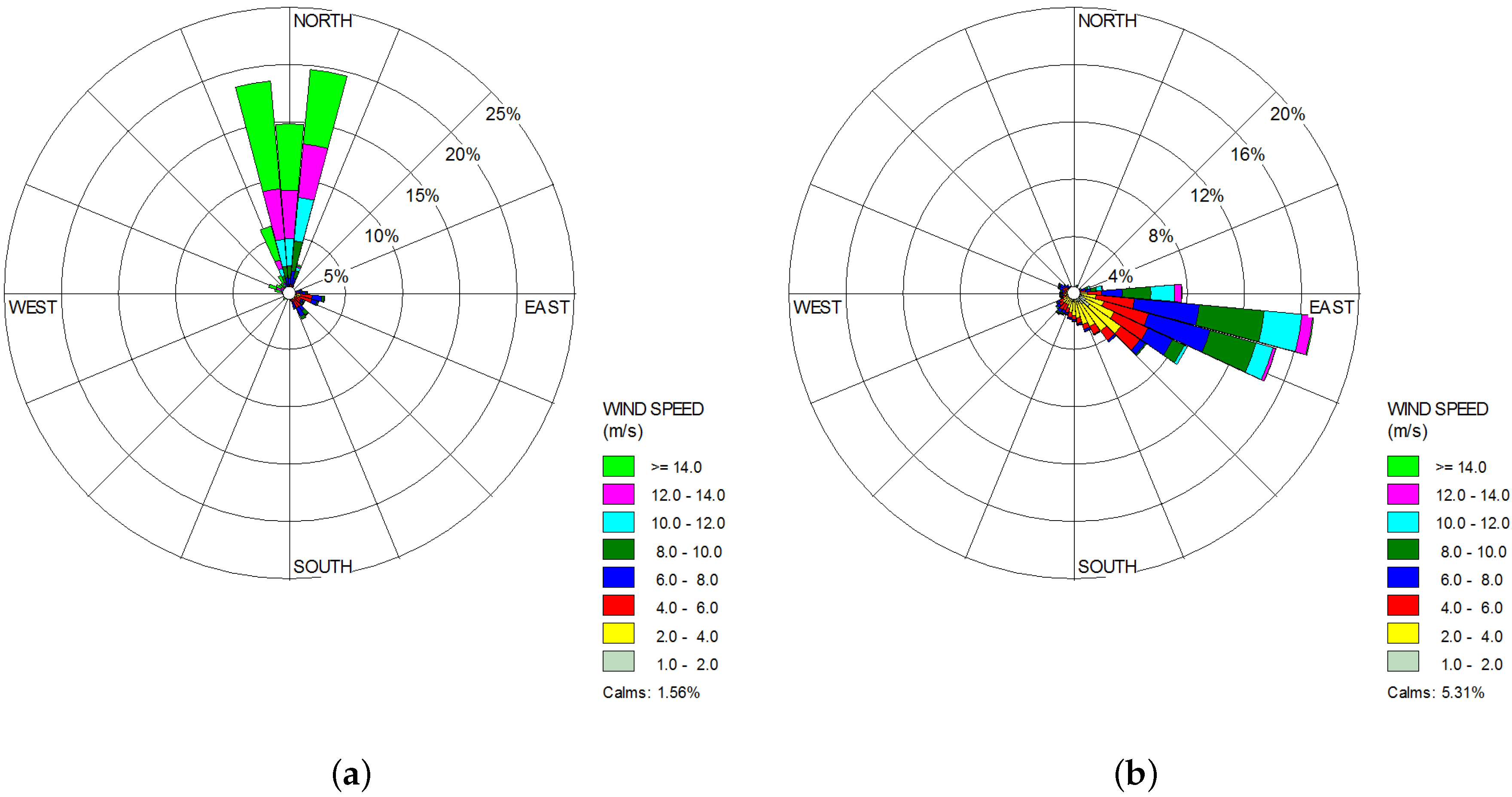
Figure 2 shows the wind rose for both sites, where $0^{\circ }$, ${90}^{\circ }$, ${180}^{\circ }$ and ${270}^{\circ }$ denote North, East, South and West directions, respectively. In the case of La Mata, Oaxaca, the dominant wind direction is from the South (S). It should be noted that the wind direction is in the range from ${335}^{\circ }$ to ${15}^{\circ }$ for $59.4\%$. Periods of calm (<1 m/s) represent $1.56\%$ of the total sample. In the case of Metepec, Hidalgo, the dominant wind direction is from West–Northwest (W–NW). It should be noted that $53.4\%$ of the time the wind directions is in the range from ${85}^{\circ }$ to ${135}^{\circ }$. Periods of calm (<1 m/s) represent $5.31\%$ of the total sample.

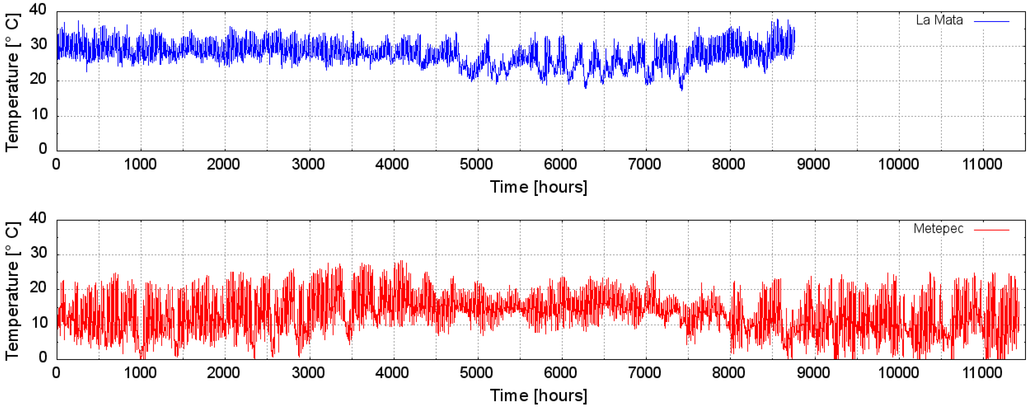
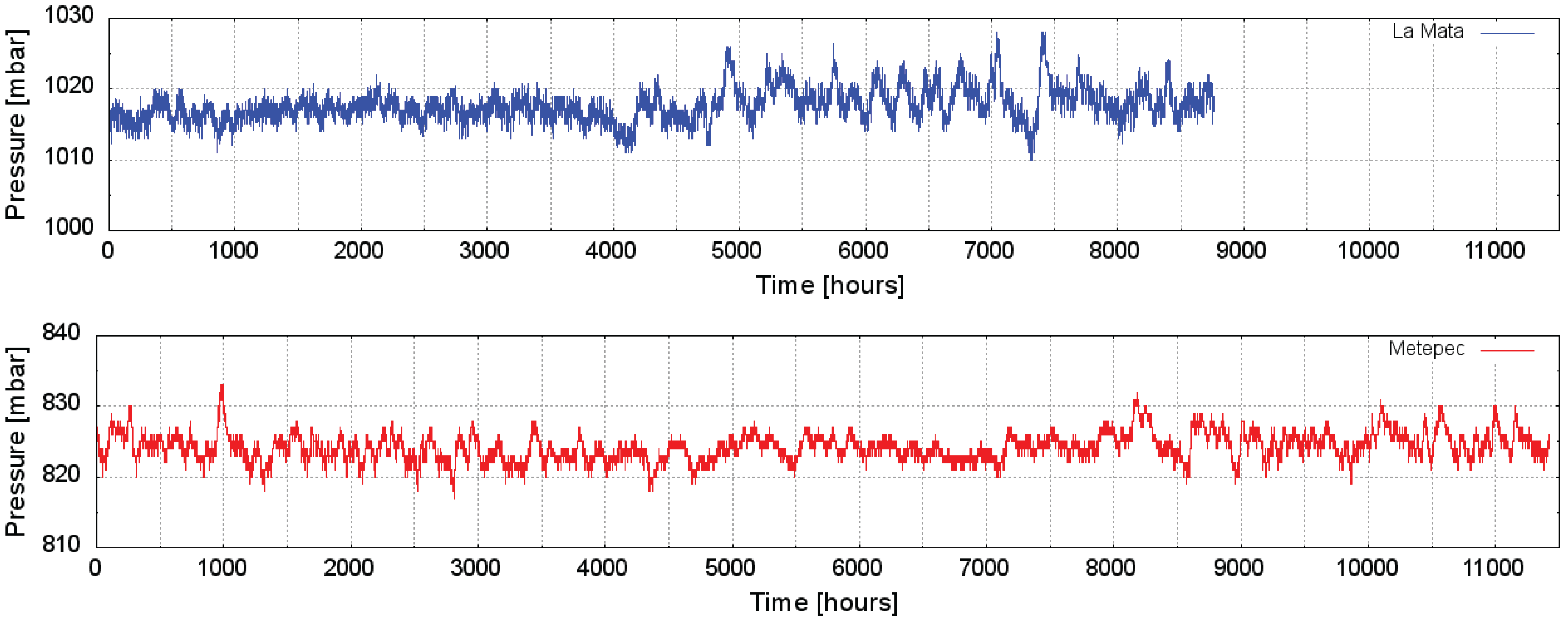
Figure 3 and Figure 4 show hourly average air temperature and barometric pressure, respectively, for both sites. The solar radiation series shown in Figure 5 for the La Mata site of course shows a daily cycle. The relative humidity for the Metepec site is shown in Figure 6.

Table 1. Descriptive statistics of the involved variables of La Mata. WS, wind speed; WD, wind direction; T, temperature; P, pressure; SR, solar radiation.

Variable	Minimum	Maximum	Mean	Mode	Standard Deviation
WS (m/s)	$0.4$	$28.3$	$10.9$	$13.6$	$5.5$
WD (${}^{\circ }$)	0	360	$4.8$	$9.5$	$36.5$
T (${}^{\circ }$C)	$17.3$	$37.9$	$27.6$	$27.2$	$3.4$
P (mbar)	1010	1028	$1017.6$	1017	$2.5$
SR (W/m${}^2$)	0	1026	$249.6$	0	$332.7$
RH (%)	−	−	−	−	−

and

Table 2. Descriptive statistics of the involved variables of Metepec. RH, relative humidity.

Variable	Minimum	Maximum	Mean	Mode	Standard Deviation
WS (m/s)	$0.4$	$19.3$	$5.2$	$0.4$	$3.2$
WD (${}^{\circ }$)	$6.6$	$355.9$	$113.3$	$103.3$	$50.5$
T (${}^{\circ }$C)	$-2.4$	$28.3$	13	$11.7$	$5.3$
P (mbar)	$817.2$	833	$824.2$	824	2
SR (W/m${}^2$)	−	−	−	−	−
RH (%)	$5.7$	$98.4$	$71.2$	$92.8$	$22.3$

give the basic statistical characteristics (Central tendency and dispersion) for each of the measured variables for La Mata and Metepec respectively. The calculation of the mean wind direction and standard deviation requires special attention because the wind direction is a circular function resulting in a discontinuity ($0^{\circ }$–${360}^{\circ }$), so that the arithmetic mean cannot be used. Therefore, the mean wind direction was calculated using the arctangent function of the averages of the sine and cosine of the wind directions data.

3. Time Series Models

A time series model ($y_t$) reproduces the patterns of the prior movements of a variable over time and uses this information to predict its future movements. It is possible in this way to construct a simplified model of the time series that represents its randomness, so that it is useful for prediction [23].

The present study uses univariate and multivariate techniques for wind speed prediction. The univariate method employs an autoregressive integrated moving average (ARIMA) model with only the wind speed as a variable. The multivariate method uses a non-linear autoregressive exogenous (NARX) model using wind direction, air temperature, barometric pressure, solar radiation and relative humidity, in addition to wind speed.

Multivariate analysis allows simultaneous consideration of diverse datasets allowing optimal decisions to be made considering all of the information.

3.1. Autoregressive Integrated Moving Average Models

ARIMA models have been used in a great number of time series prediction problems, because they are robust, as well as easy to understand and implement. However, difficulties exist with atypical values influencing the estimation of future values. A further disadvantage of stochastic models is generally their high order.

In the early 1970s, ARIMA models were popularized by Box and Jenkins [24], their names being associated with general ARIMA models applied to time series analysis and forecasting.

There are many ARIMA models. The non-seasonal general model is known as ARIMA(p,d,q), where:

• AR:p = order of the autoregression of the model;
• I:d = degree of differencing to make the model stationary;
• MA:q = order of the moving average aspect of the model.

The linear expression to define the above notation is:

$$y_t=\sum _{i=1}^p{\varphi }_i{y}_{t-i}+\sum _{j=1}^p{\theta }_j{e}_{t-i}+{ϵ}_t$$

(1)

where ${\varphi }_i$ for the purpose of stabilizing the variance, ${}_i$ is the i-th autoregressive parameter, ${\theta }_j$ is the j-th moving average parameter and ${ϵ}_t$ is the error term at time t.

ARIMA models are used in a wide range of applications from engineering to economics. In cases such as the prediction of power demand, wind speed and stock market value behavior, that is things that can be represented as a time series with sufficient measurements, these can be modeled by this technique.

The Box-Jenkins method was followed to model the time series from La Mata and Metepec. This is basically a three-step iterative process: model identification, parameter estimation and diagnostic checking [24]:

• Identification. Identification methods are approximate procedures applied to a dataset to find the kind of model worth further investigation. This involves determining suitable values for parameters p and q and determining the degree of differencing, d, to obtain stationarity. At this stage, graphs of the original and differenced time series together with their estimated autocorrelation and partial autocorrelation functions are useful tools.
• Estimation. Having an initial model specification, its parameters are estimated from the maximum likelihood or conditional least squares methods. These are used iteratively starting from values estimated during the identification stage.
• Diagnostic Checking. Having identified the model and estimated its parameters, diagnostic checks are used to reveal its inadequacies and indicate suitable improvements. Residuals and their autocorrelations are inspected. If the model is a good fit to the data, then the residuals would correspond to white noise and have very little autocorrelation.

Proposed ARIMA Models

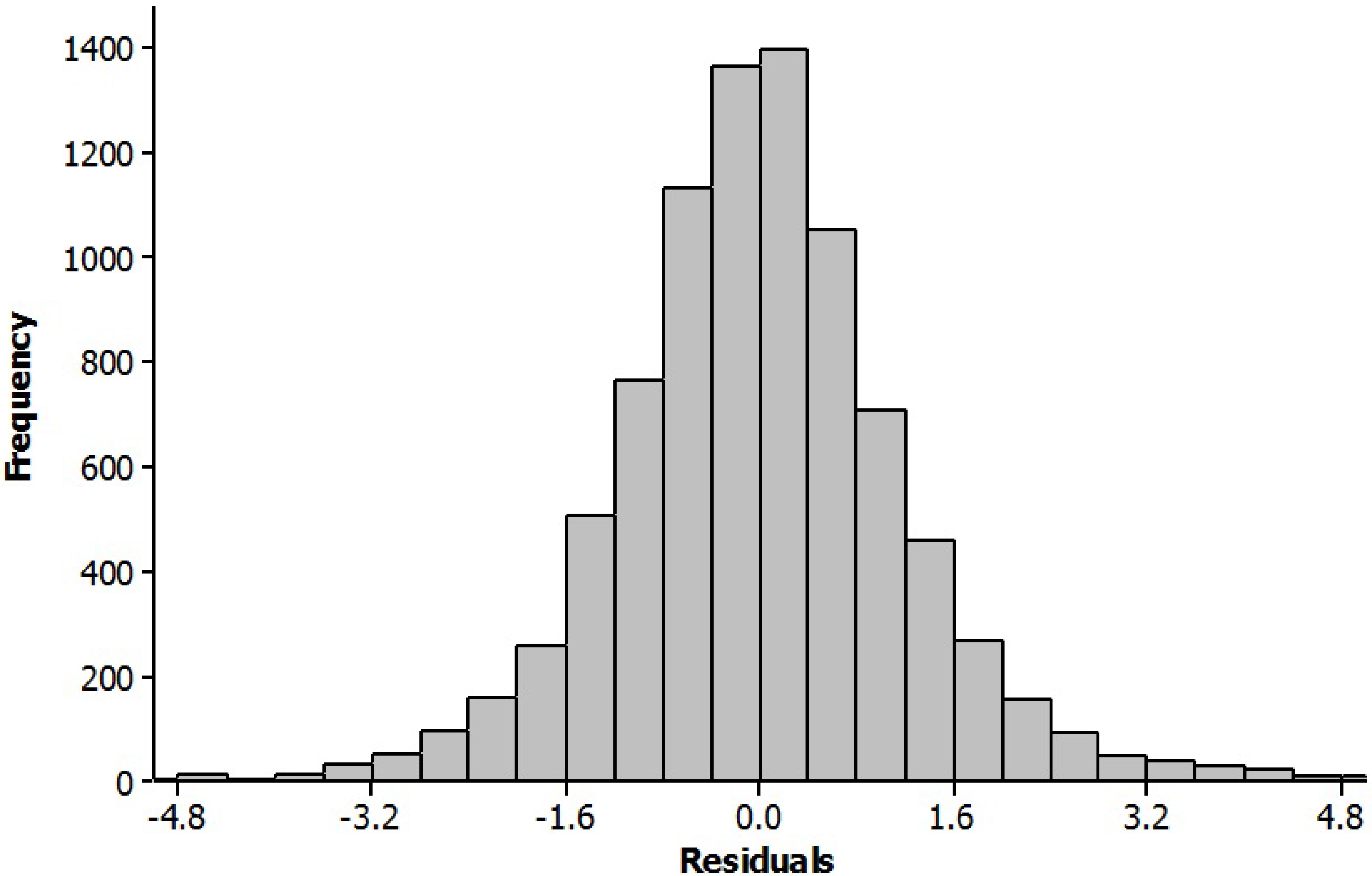
As described above, in the Identification step, the data were differenced to obtain a stationary or trend-free series (Figure 7). A transformation of the original series was obtained to stabilize the mean and variance and to identify potential models from the autocorrelation function (ACF) and the partial autocorrelation function (PACF). At this stage of data preparation, it was determined whether or not it should be transformed to stabilize the variance. In the following Estimation step, the parameters in potential models were calculated, and suitable criteria were used to select the best model (Figure 8). Finally, ACF and PACF were used to test the residuals as the Diagnostic Checking stage. Normality and “t” tests were applied to the residuals to find their closeness to white noise (Figure 9 and Figure 10).

For La Mata and Metepec, the ARIMA models were ARIMA(1,1,0) and ARIMA(1,1,1), respectively.

Table 3. ARIMA models for the two studied sites.

Site	ARIMA$(p,d,q)$	Model
La Mata	ARIMA$(1,1,0)$	$y_t=1.1y_{t-1}-0.1y_{t-2}$
Metepec	ARIMA$(1,1,1)$	$y_t=0.3742y_{t-1}+0.6258y_{t-2}+0.6601e_{t-1}+e_t$

shows the details of each of the two models. In the case of La Mata, the coefficient corresponding to the first term of equation: $1.1y_{t-1}$ indicates the importance of the wind speed one hour earlier. This shows that the wind speed is persistent in this region. In the case of Metepec, the second term of the model apparently has a higher relevance: $0.6258y_{t-2}$; however, the third term, the error coefficient $0.660e_{t-1}$, which only involves a delay, has a similar order of magnitude. These two terms are thus of similar importance.

Histograms of the residuals between the models and the measured time series for La Mata and Metepec are shown in Figure 9 and Figure 10, respectively. The histograms show the form of the residuals’ distribution. It can be seen qualitatively that both cases are sharp normal distributions. The Metepec database has a lower scatter and higher frequencies because of the larger dataset. Both histograms are symmetrical, and this is borne out by the measures of central tendency, such as the mean, median and mode coinciding. This shows that there are no other patterns present in the data.

3.2. Nonlinear Autoregressive with Exogenous Inputs Models

The NARX model is a type of dynamically-driven recurrent ANN. Recurrent networks have one or more feedback loops, which can be either local or global. Global loops reduce the computational memory requirements. There are two basic uses for recurrent networks:

• associative memory;
• input-output mapping networks.

Two applications of input-output are signal modeling and prediction in the form of time series. The most obvious advantage of the NARX models is that the same structure makes up different models and it thus has a reasonable computation cost. Thus, a NARX network can gain degrees of freedom when it includes a time period forecast as an input for subsequent periods compared to a feedforward network. This allows summary information of exogenous variables to be included, as well as a lesser number of residuals, which reduces the number of parameters that have to be estimated.

NARX networks have a more effective learning process compared to other types of neural networks (the learning gradient descent is better). These networks converge, and generalization is improved compared to other types of networks [25].

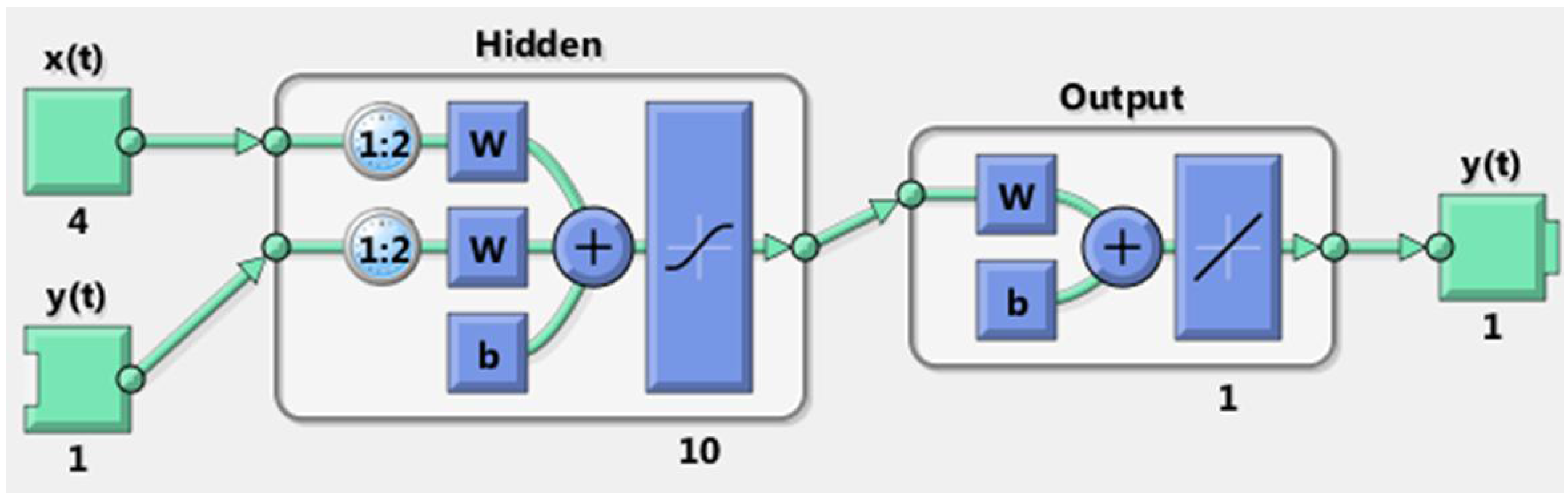
Figure 11 shows the simplest architecture for a NARX model. The model in this case has only one input, which represents the value of the exogenous variables, which in turn provides feed-forward to a q number of delayed memory neurons. It has only one output $y(t+1)$, which represents the value of the predicted variable one step ahead. In other words, the output is one time unit ahead of the input. In turn, the output provides feedback to the network through a number of q delayed memory neurons.

These two lines make up the input neural layer of a multilayer perceptron [26]. The following expression describes the model’s dynamic behavior:

$$y(n+1)=F\left(y\left(n\right),\cdots ,y(n-q+1),u\left(n\right),\cdots ,u(n-q+1)\right)$$

(2)

where F is a nonlinear function of its arguments.

3.2.1. Learning Algorithm for the NARX Network

The neurons in the NARX models are sigmoid, and the performance function used in the training of the ANN is the mean squared error (MSE). For the NARX network, it is replaced as follows:

$$MSE=\frac{1}{n}\sum _{i=1}^n{\left(e_i\right)}^2=\frac{1}{n}\sum _{i=1}^n{(t_i-y_i)}^2$$

(3)

$$MSW=\frac{1}{n}\sum _{j=1}^n{\left(W_i\right)}^2$$

(4)

$$MS{E}_{reg}=\gamma ·MSE+(1-\gamma )·MSW$$

(5)

where: $t_i$ = target, γ = performance ratio and $MSW$ = mean squared weight.

This performance function results in smaller weights and biases in the network and, thus, makes the response smoother and less likely to over fit. The training function that updates the weights and bias values uses Levenberg–Marquardt optimization, which was modified to include the regularization technique [27].

3.2.2. Proposed NARX Models

The NARX model that had the best forecast performance used five input variables with two delays per variable. These were wind speed and direction, air temperature, barometric pressure and solar radiation (for La Mata) or relative humidity (for Metepec). There were ten hidden neurons. The final configuration is shown in Figure 12.

3.3. Statistical Error Measures

The models’ performance was evaluated via statistical error measurements. These were mean absolute error (MAE), mean squared error (MSE) and mean absolute percentage error (MAPE), described by the following expressions:

$$MAE=\frac{1}{n}\sum _{t=1}^n\left|e_t\right|$$

(6)

$$MSE=\frac{1}{n}\sum _{t=1}^n{e}_t^2$$

(7)

Hindcasts are a way of evaluating the difference between model results and measurements. The MAE is a measure of the average of the absolute error whose advantage is that it is easier for non-specialists to understand. MSE is similar, but the values are all positive due to the squaring; this makes it easier to use in an optimization technique [28]. To achieve a higher degree of certainty when comparing models, the MAPE was calculated by means of the percentage error ($P{E}_t$) and the mean percentage error (MPE) using the following expressions:

$$P{E}_t=\left(\frac{Y_t-F_t}{Y_t}\right)·100$$

(8)

$$MPE=\frac{1}{n}\sum _{t=1}^{n}P{E}_t$$

(9)

$$MAPE=\frac{1}{n}\sum _{t=1}^n\left|P{E}_t\right|$$

(10)

The MAPE makes the comparison of results between from the two models easier because it is percentage based. This gives an indication of the size of the prediction errors in comparison to the measured values in the series.

4. Wind Speed Forecasting Results

Two different sites were selected to demonstrate the effectiveness of the methods proposed for wind speed forecasting and to verify the influence of other atmospheric variables besides wind speed on their accuracy. Each dataset was divided into three parts: $70\%$ for training, $15\%$ for validation and $15\%$ for testing.

Table 4. Datasets for the forecasting analysis.

Site	Training Set	Validation Set	Testing Set	Total Data
	(70%)	(15%)	(15%)	(100%)
La Mata	6131	1314	1314	8759
Metepec	47,994	10,278	10,278	68,550

shows the details of these datasets.

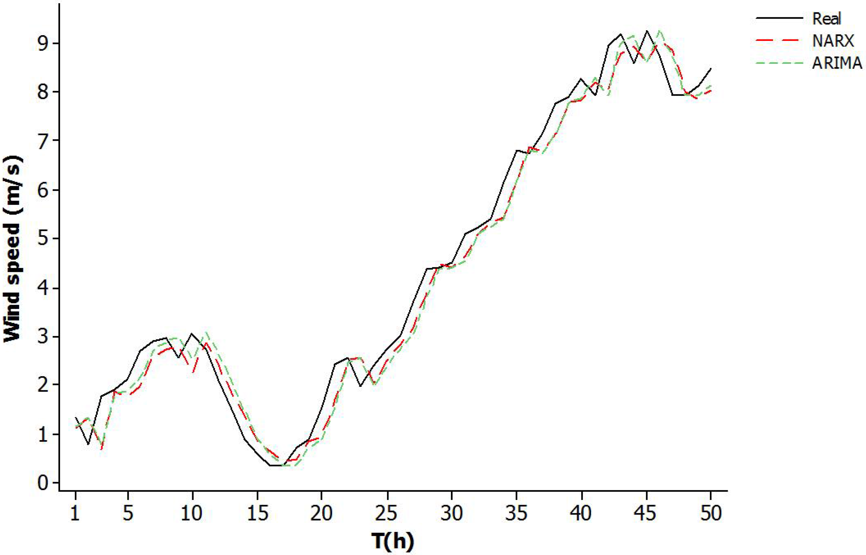
To see how the prediction models fit to the real data, Figure 13 and Figure 14 show the last 50 h of data allowing a qualitative comparison. These correspond to 50 data points for La Mata and 300 for Metepec. In these figures, the solid curve is the measured data, the long dashed curve is the ARIMA modeling and the shorter dashed curve is the NARX modeling. From these figures, the importance of the meteorological values of the previous time step (previous hour for La Mata and previous 10 min for Metepec) is obvious for one step ahead wind speed prediction, indicating the persistence of the wind speed on the short-term for these sites.

The mean absolute error and the mean squared error were used to quantitatively evaluate which model best predicts the wind speed behavior.

Table 5. Statistical errors generated by the ARIMA and NARX models.

Model	La Mata		Metepec
	MAE	MSE	MAE	MSE
ARIMA	$0.91$	$1.51$	$0.44$	$0.39$
NARX	$0.86$	$1.35$	$0.43$	$0.34$
Improved Percentages	$5.5\%$	$10.6\%$	$2.3\%$	$12.8\%$

shows these measures of forecasting error. The improvement of the NARX model over the univariate ARIMA model based on the MAE and MSE results was calculated using the following equations:

$$P_{MAE}=\left|\frac{MA{E}_{ARIMA}-MA{E}_{NARX}}{MA{E}_{ARIMA}}\right|·100$$

(11)

$$P_{MSE}=\left|\frac{MS{E}_{ARIMA}-MS{E}_{NARX}}{MS{E}_{ARIMA}}\right|·100$$

(12)

From Figure 13 and Figure 14, it can be seen that both models are effective, but it is not obvious which is the best. The error measures in Table 5 confirm the satisfactory performance of both models; however, it is clear that the NARX model is significantly better than the ARIMA model. The MAE of the NARX model for La Mata is $5.5\%$ better than the ARIMA model and $2.3\%$ better for Metepec. The MSE percentage improvements are better than for MAE with values of $10.6\%$ and $12.8\%$ for La Mata and Metepec, respectively.

The additional information provided by more meteorological variables and the non-linear nature of the multivariate NARX model explain the superiority of this model.

5. Conclusions

A procedure to analyze and predict wind speed using standard meteorological variables was developed. Firstly, using traditional statistical techniques, such as the ARIMA model, and, secondly, by using a multivariate artificial neural network technique: the NARX model. Wind speed predictions given by both models were analyzed and compared qualitatively and quantitatively with measured data.

The results obtained show reasonable one step ahead wind speed prediction can be made with the univariate ARIMA model. However, by using a multivariate NARX model, more accurate results were obtained. The inclusion of additional meteorological variables is thus recommended in wind speed forecasting models if they are available.

As well as being a multivariate model, the NARX neural network is a class of discrete-time non-linear techniques that can represent a variety of non-linear dynamic systems, as in the case of wind speed time series.