Investigation of a High Head Francis Turbine at Runaway Operating Conditions

Abstract

Hydraulic turbines exhibit total load rejection during operation because of high fluctuations in the grid parameters. The generator reaches no-load instantly. Consequently, the turbine runner accelerates to high speed, runaway speed, in seconds. Under common conditions, stable runaway is only reached if after a load rejection, the control and protection mechanisms both fail and the guide vanes cannot be closed. The runner life is affected by the high amplitude pressure loading at the runaway speed. A model Francis turbine was used to investigate the consequences at the runaway condition. Measurements and simulations were performed at three operating points. The numerical simulations were performed using standard k-ε, k-ω shear stress transport (SST) and scale-adaptive simulation (SAS) models. A total of 12.8 million hexahedral mesh elements were created in the complete turbine, from the spiral casing inlet to the draft tube outlet. The experimental and numerical analysis showed that the runner was subjected to an unsteady pressure loading up to three-times the pressure loading observed at the best efficiency point. Investigates of unsteady pressure pulsations at the vaneless space, runner and draft tube are discussed in the paper. Further, unsteady swirling flow in the blade passages was observed that was rotating at a frequency of 4.8-times the runaway runner angular speed. Apart from the unsteady pressure loading, the development pattern of the swirling flow in the runner is discussed in the paper.

1. Introduction

Hydraulic turbines are used extensively to stabilize power grids, because they can restart rapidly and/or change the power output according to the real-time demand. In recent years, a continuous increase in grid-connected wind and solar power has resulted in problems related to power grid stability and reliability. There have been an increasing number of incidents of power fluctuations in the grid network [1]. When the grid parameters fluctuate beyond a manageable limit, the generator of the hydraulic turbine automatically disconnects from the grid, resulting in an unexpected transition into no load conditions (i.e., total load rejection). Consequently, the turbine runner accelerates to a runaway speed within a few seconds [2,3]. The runaway speed is generally more than 150% of the synchronous speed. However, the acceleration rate for axial and other radial flow turbines may vary because this rate depends on the rotating masses, the load and the operating condition. Under common conditions, stable runaway is only reached if after a load rejection, the control and protection mechanisms both fail and the guide vanes cannot be closed. At the runaway condition, the runner is subjected to a very high amplitude unsteady pressure loading and significant vibrations that cause the blades to fatigue [4,5,6,7,8].

Studies [2,6,7,9,10] on hydraulic turbines during total load rejection have shown that the runner was subjected to an unsteady pressure loading with an amplitude that was more than twice that at the normal operating condition, i.e., the best efficiency point (BEP). The amplitudes and frequency of the pressure fluctuations are primarily attributed to the rotor stator interaction (RSI), which increases with the runner angular speed. This speed rise condition may be observed for a few seconds because the guide vanes close rapidly after total load rejection [2]. However, the closing rate depends on the operating point, the inertia of the rotating masses and the time available to prevent water hammer. The closing rate of the guide vanes significantly affects the transient pressure loading in the runner.

At the runaway condition, unsteady swirling flow develops for which the discharge is extremely low, and the runner rotates at high speed. This flow results in high-amplitude unsteady pressure fluctuations on the blade surfaces. Unsteady pressure measurements on a Francis turbine [11,12,13,14,15,16] have shown that a small opening of the guide vanes and high angular speed of the runner induced largely separated flow at the runner inlet. The pressure difference between the pressure and suction sides of the blades increases, which results in an increase of the runner speed. Experimental and numerical studies on pump-turbines at the runaway condition showed that the flow instabilities at the runner inlet resulted in unstable flow, e.g., the continuous formation and destruction of large eddies [17].

The literature [4] on current operating trends for the hydraulic turbine shows that the total load rejection and the runaway condition cause significant damage to the turbine runners. Damage due to cyclic fatigue is equivalent to the several hours of runner operation at BEP [18,19,20]. The rotor deformation is also one of the main concerns, as there is a danger of touching in the labyrinth seals and generator gaps. However, this work focuses on the flow field; the mechanical consequences are not addressed in this paper.

In the present study, we primarily focus on experimental and numerical studies of the flow field and its effects on the runner blades at the runaway condition. Three operating points of a model Francis turbine were selected. The time-dependent pressure measurements were carried out using pressure sensors located at the vaneless space, the runner and the draft tube. The experimental results were used to validate the numerical model, which were then used to analyze the flow further.

2. Test Rig and Instrumentation

A scaled model of a high head Francis turbine (D_P = 1.78 m, H_P = 377 m, Q_P = 31 m³·s⁻¹, N_QE = 0.27) was used in the experimental studies. The turbine included 14 stay vanes that were integrated into the spiral casing, 28 guide vanes, a runner with 15 blades and 15 splitters and an elbow-type draft tube. The reference diameter (D_M) was 0.349 m. The total, random and systematic, uncertainty in the hydraulic efficiency was ±0.16% at the BEP, based on calibration of the instruments before the measurements. The calibration and uncertainty computation were performed using the procedure available in IEC 60193 [21].

The test rig was operated with an open-loop hydraulic system to obtain a condition similar to the prototype without a significant variation of the available head during the measurement. Water from the large basement was continuously pumped to the overhead tank and flowed down to the turbine. The pump was operating at constant speed, and the water above a certain height (H_M ≈ 12 m at BEP) in the overhead tank flowed down to the basement. The measured pressure head at the turbine inlet was 220 kPa absolute at the BEP. The draft tube outlet was connected to the downstream tank, where a constant water level was maintained (equal to the level of the runner outlet), and water above this level was discharged to the basement. The tank was open at atmospheric pressure, and the draft tube was submerged under the constant water level. The laboratory area of the basement is large compared to the discharge in the model turbine; therefore, there was negligible variation in the water temperature, and the maximum water temperature was 15.6 °C. A minimum pressure of 80 kPa was recorded at the blade trailing edge, which is much higher than the vapor pressure of the water. Therefore, the measurement condition was believed to be cavitation free.

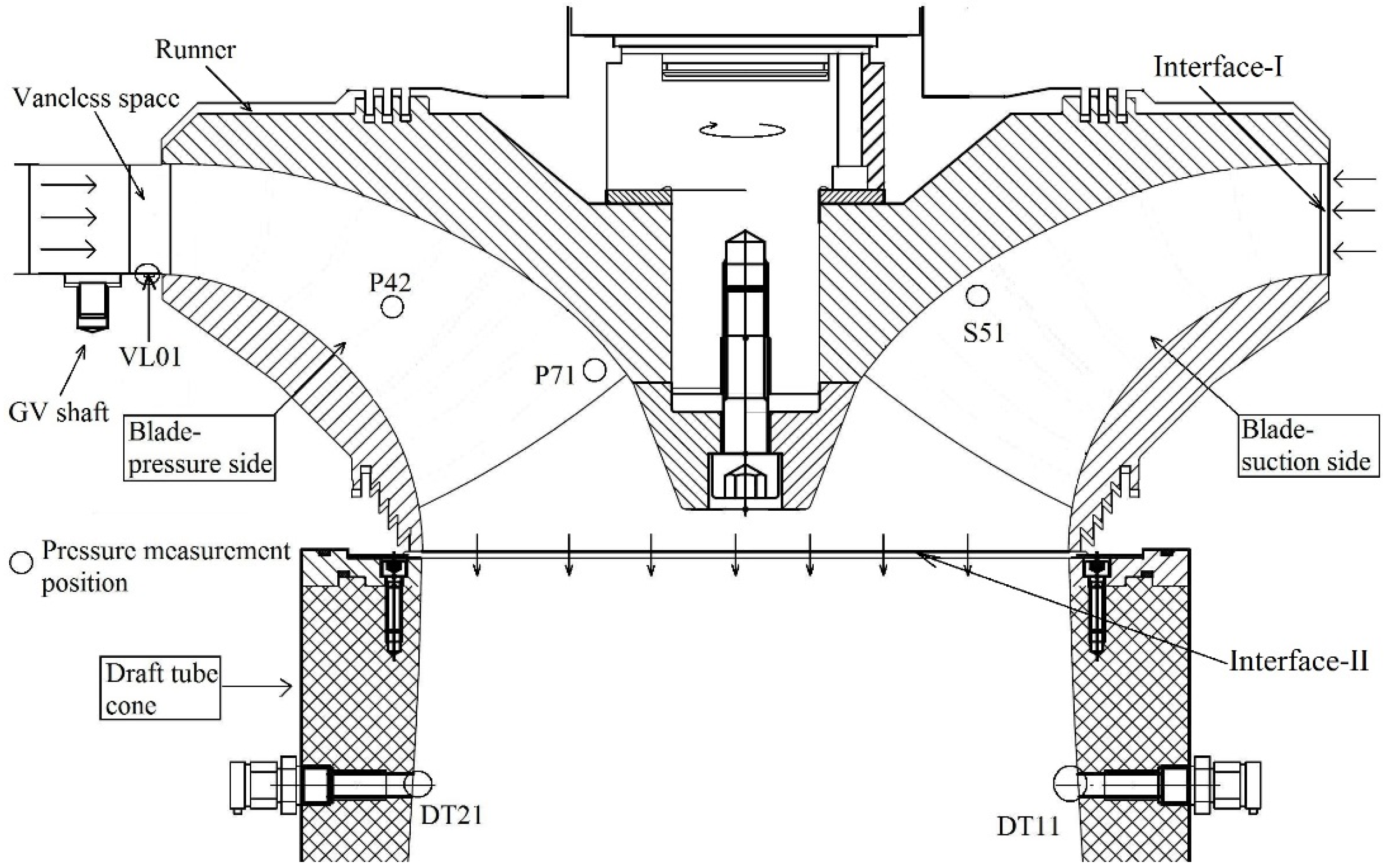
A total of eight pressure sensors were used for unsteady pressure measurement. Two pressure transmitters, PTX1 and PTX2, were located at the turbine inlet pipe. PTX1 and PTX2 were flush with the pipe surface and located at 4.87 and 0.87 m, respectively, from the inlet of the spiral casing. The other six sensors were located in the turbine (see Figure 1). A sensor (vaneless space (VL01)) was integrated on the surface of the bottom ring in the vaneless space, a gap between the guide vanes row and the runner, to capture the effect of rotor stator interaction. Three miniature-type sensors, P42 (blade pressure side), P71 and S51 (blade suction side), were integrated on the runner blade surfaces at the pressure side, the trailing edge and the suction side, respectively. Data from the runner sensors were acquired using a wireless telemetry system, Summation Research SRI-500e. The remaining two sensors, DT11 (draft tube cone) and DT21, were mounted to the wall of the draft tube cone. Both sensors were located 180° radially apart from each other at the same axial position (h^* = 1.7). The dimensionless axial and radial positions of the sensors are listed in

Table 1. Dimensionless radial and axial positions of pressure sensors mounted in the turbine; reference radial distance (R_M) = D_M/2 = 0.1745 m; h_ref = 0.1794 m.

Sensor	Stationary Domain			Rotating Domain
	VL01	DT11	DT21	P42	P71	S51
r* = r/RM	1.87	1.04	1.04	1.02	0.45	0.66
h* = h/href	0.16	1.70	1.70	0.29	0.48	0.28

. The axial position (h) was measured from the midpoint of the breadth of the runner inlet, and the radial position (r) was measured from the runner rotation axis. The reference radial distance (R_M) was the radius measured at the runner outlet, i.e., D_M/2. The reference axial distance (h_ref) was considered as the runner depth, i.e., the midpoint of the breadth of the runner inlet to the runner outlet.

The measurements were divided into two parts: (i) evaluation of the performance characteristics, and (ii) evaluation of the runaway characteristics. A constant efficiency hill diagram was constructed to evaluate the turbine performance under normal operating conditions. A maximum hydraulic efficiency of 93.4% was observed for a guide vane angle (α) of 9.9°, a runner angular speed (n) of 335.9 rpm, a net head (H) of 11.9 m and a discharge (Q) of 0.2 m³·s⁻¹. This condition is regarded as BEP in the paper. A detailed analysis of the performance characteristics has been discussed in a previous publication [4].

Three angular positions of the guide vanes were used for the measurements at the runaway condition: 3.9°, 9.9° and 12.4°. A frequency controller coupled to the generator was used to increase the runner angular speed. The speed was increased until the shaft torque reached zero, while maintaining the same position of the guide vanes, i.e., 3.9°. A similar procedure was followed for the other two angular positions of the guide vanes.

Table 2. Operating parameters and specific hydraulic energy (ρE) for runaway and BEP operating conditions.

Cases	Runaway Condition			BEP
	I	II	III
α (°)	3.9	9.9	12.4	9.9
nR (Hz)	8.12	8.74	8.84	5.53
QR (m3·s−1)	0.047	0.080	0.088	0.200
nED (–)	0.257	0.278	0.281	0.180
QED (–)	0.035	0.059	0.065	0.150
HM (m)	12.38	12.27	12.25	11.91
ρE (kPa)	121.48	120.40	120.20	116.84
Re (–)	2.8 × 106	3 × 106	3.02 × 106	1.88 × 106

summarizes the observed parameters at the runaway and BEP conditions. The runaway speed (n_R) for all of the points was more than 150% of the turbine synchronous speed (n) at BEP, i.e., 5.53 Hz. The runaway speeds for the angular positions of the guide vanes at 3.9°, 9.9° and 12.4° were 8.12, 8.74 and 8.84 Hz, respectively. The discharge (Q_R) was lower at the runaway conditions than at the BEP, as expected. At the constant angular position of 9.9°, the discharge values at the runaway and BEP conditions were 0.08 and 0.2 m³·s⁻¹, respectively. The shaft torque (T), i.e., the torque to the generator, was almost zero at all of the runaway points. The shaft torque at the BEP was 621 N m, i.e., 75% of the maximum load. The Reynolds numbers were 2.8 × 10⁶ to 3.02 × 10⁶ during the runaway conditions.

3. Numerical Model

3.1. Computational Domain

The commercial software ANSYS was used to create the geometry and mesh in the turbine. The computational domain is shown in Figure 2. The domain included three sub-domains, a distributor, a runner and a draft tube. The inlet and outlet boundary locations are identical to the actual measurement locations. The mass flow inlet boundary was prescribed at the casing inlet, and an opening type boundary condition with static pressure was prescribed at the draft tube outlet. The entrainment static pressure at the draft tube outlet was prescribed. The advantage of this boundary condition is that it allows recirculating flow at the draft tube outlet. General grid connection Type 2 interfaces were used to connect the rotating domain. Interface-I was placed between the distributor and runner. Interface-II was placed between the runner and the draft tube.

Three turbulence models, standard k-ε, shear stress transport (SST) and scale-adaptive simulation (SAS), were used to resolve/model the flow [17,18,19,20,21,22]. A high resolution scheme was enabled to calculate the advection terms in the discrete finite volume equations. A backward Euler, second-order accurate, implicit time-stepping scheme was enabled for the unsteady analysis. The total simulation time was two seconds, which was equivalent to 15 revolutions of the runner. The final simulation was initialized with the unsteady simulations performed with the SST model for one second. The periodical flow condition was observed after one complete rotation of the runner. The time step size and convergence criteria were selected considering information available in the literature [4,5,6,7,8,9,10,11,12,13,14,15,16,17,18,19,20,21,22]. The convergence criteria for the mass, momentum and turbulence parameters were set to a root-mean-square (RMS) value less than 1 × 10⁵. The selected inner loop iteration for the transients at each time step was 10. The solution was converged at each time step within five inner loop iterations.

Continuous blocks of a hexahedral mesh were constructed in each domain to prevent local interfaces from forming inside the sub-domains. A hexahedral mesh was employed for all of the domains. Figure 3 shows the mesh that was constructed in the distributor and part of the runner. A dense mesh can be seen in complex passages, such as the guide vanes row, the inlet to the runner, the leading edge of the blade, etc. After the mesh scaling test, a total of 12.8 million nodes of hexahedral mesh elements were used for the turbine. Before the simulations were performed at the runaway operating condition, the mesh scaling tests and mesh performance tests were carried out. The scaling tests were carried out at the BEP operating condition of the turbine. The detailed results of the scaling test have been presented in a previous publication [4].

3.2. Grid Scaling Test

Table 3. Mesh densities used in scaling test and quality parameters [4].

Grid Type	G1	G2	G3
Distributor	8,528,119	3,255,676	2,073,735
Runner	7,527,320	4,047,898	1,766,246
Draft tube	4,679,404	3,639,241	991,512
Total nodes (millions)	20.73	12.84	4.83
Minimum angle	38	41	23
y+ (BEP)	≤40	≤65	≤285

shows the three different grid densities (fine, G₁; medium, G₂; and coarse, G₃) that were used for the scaling test. The G₃-type mesh was the coarsest mesh in the simulation. The subsequent mesh was updated in the i, j and k directions. The grid quality was refined at each step of grid creation so that the mesh nodes did not correspond exactly to a 2× increase. As the main focus of the present investigation was in the runner domain, the maximum number of nodes and the quality of the grid were maintained in the runner. The minimum angle of the elements for the fine, medium and coarse grids was 38, 41 and 23, respectively.

The widely-accepted grid convergence index (GCI) method was used to evaluate the grid convergence. A method described by Celik [23] was used:

(i) The average mesh or grid size G of a cell in the domain is represented as:

$$G={\left[\frac{1}{N}{\displaystyle \sum _{i=1}^N\left(\Delta V_i\right)}\right]}^{\frac{1}{3}}$$

(1)

where $\Delta V_i$ is a cell volume and N is the total number of elements used for the simulation.

(ii) Simulations with three different densities of grids were performed for determining GCI. In this paper, the pressure at three locations, VL01, P42 and DT11, and hydraulic efficiency were considered as a variable, $\mathsf{\varphi }$, for the computation of GCI.

(iii) The grid refinement factor (r) was computed as $r=G_{\mathrm{fine}}/G_{\mathrm{coarse}}$, r > 1.3.

(iv) Let G₁ < G₂ < G₃ and r₂₁ = G₂/G₁, r₃₂ = G₃/G₂.

(v) The extrapolated values were calculated,

$${\mathsf{\varphi }}_{ext}^{21}=\frac{\left(r_{21}^m{\mathsf{\varphi }}_1-{\mathsf{\varphi }}_2\right)}{\left(r_{21}^m-1\right)}$$

(2)

$${\mathsf{\varphi }}_{ext}^{32}=\frac{\left(r_{32}^m{\mathsf{\varphi }}_2-{\mathsf{\varphi }}_3\right)}{\left(r_{32}^m-1\right)}$$

(3)

(vi) An approximate relative error was computed using Equation (4),

$$e_a^{21}=\left|\frac{{\mathsf{\varphi }}_1-{\mathsf{\varphi }}_2}{{\mathsf{\varphi }}_1}\right|$$

(4)

(vii) Extrapolated relative error as,

$$e_{\mathrm{ext}}^{21}=\left|\frac{{\mathsf{\varphi }}_{ext}^{21}-{\mathsf{\varphi }}_2}{{\mathsf{\varphi }}_{\mathrm{ext}}^{21}}\right|$$

(5)

(viii) The GCI was computed for the fine to medium grid as,

$$GC{I}_{\mathrm{fine}}^{21}=\frac{1.25\cdot e_a^{21}}{r_{21}^2-1}$$

(6)

Table 4. Discretization error and uncertainties in numerical solutions [4].

Parameter	VL01	P42	DT11
r21	1.39	1.39	1.39
r32	1.33	1.33	1.33
G1 (kPa)	178.23	123.83	99.70
G2 (kPa)	176.37	123.73	99.64
G3 (kPa)	176.32	123.55	99.64
$G_{\mathrm{ext}}^{21}$ (kPa)	180.20	123.95	99.76
$e_a^{21}$	0.0104	0.0008	0.0005
$e_{ext}^{21}$	0.0109	0.0009	0.0006
$GC{I}_{\mathrm{fine}}^{21}$	0.0138	0.0011	0.0007
$GC{I}_{\mathrm{med}}^{32}$	0.0366	0.0022	0.0001

shows the computed flow parameters based on the above procedure to determine the GCI. The pressure variation at the runner outlet locations DT11 and DT21 was observed to be periodically uniform after two revolutions of the runner for a time step of 0.5°. Lower uncertainties were obtained using the medium grid density, particularly for the pressures at the runner at P42 (0.2%) and the draft tube at DT11 (0.005%). The estimation was based on a global average order of accuracy with a high resolution scheme. The apparent order of the solution ranged from 1.34 to 8.33. The pressure variation in the turbine was the critical parameter; thus, the numerical pressure was validated using the experimental values at VL01, P42 and DT11. The GCI from G₂ to G₁ was very low compared to that from G₃ to G₂. A very small difference between the medium and fine grid was observed. The converged solution obtained using the medium grid was used in subsequent simulations at different operating conditions. Simulation at one operating condition takes 25 days with 192 processors. Therefore, an optimum approach was considered for further simulations, and the medium grid was selected.

3.3. Mesh Performance under Normal Operating Conditions

The simulations for the mesh performance were carried out at five operating points. The performance of the numerical model during normal operating conditions is shown in Figure 4. The difference between the experimental and numerical hydraulic efficiency is shown. The maximum difference between the experimental and numerical efficiencies was observed at a low discharge (Q = 0.07 m³·s⁻¹, α = 3.91°) operating condition. The numerical hydraulic efficiency (standard k-ε) was 11.44% higher than the experimental efficiency. The lowest difference between the experimental and numeric results was 0.85% at the BEP (Q = 0.20 m³·s⁻¹ and α = 9.84°). The difference between the experimental and numerical efficiencies at the high discharge operating point (Q = 0.22 m³·s⁻¹, α = 12.44°) was 2.87%. The SST k-ω model showed even a larger difference at all of the operating points. No difference for the second order advection scheme was seen with respect to the high resolution scheme.

Overall, the selected turbulence models and mesh showed satisfactory performance. Better performance at BEP could be associated with the stable flow condition where the flow is expected to be attached. At operating conditions away from BEP, the turbulence models showed some difficulty in capturing the unsteady flow features. The models underestimated the losses, predicting a higher efficiency. The highest difference between the experimental and numerical results that were obtained at part load may be attributed to the difficulty of capturing the vortex breakdown that occurred in the draft tube cone.

The numerical hydraulic efficiency is higher than the corresponding experimental values at all of the operating points. The labyrinth seals at the runner crown and the band sides are not modeled; therefore, the numerical hydraulic efficiency does not account for the losses from leakage that generally occur during measurements. The mesh for the angular positions of 3.9°, 9.9° and 12.4° of the guide vanes was used for the simulations performed at the runaway operating condition. Apart from standard k-ε and SST k-ω models, a hybrid Reynolds-averaged Navier-Stokes equations-Large Eddy Simulation RANS-LES turbulence model (SAS-SST) was employed for the runaway simulations. The hybrid model is based on the von Karman length scale for blending function formulation. Therefore, it is expected that this model will capture the unsteady flow features in the runner. The performance of this model was evaluated extensively by several authors for similar flow conditions [22,24,25,26,27].

4. Results and Discussion

4.1. Average Pressure Loading

The experimental and numerical pressure values were compared at the sensor locations in the turbine. To obtain the numerical pressure values, six monitoring points were created that corresponded to the locations, VL01, P42, S51, P71, DT11 and DT21. Equation (7) was used to compute the pressure coefficient at the sensor locations at each operating point.

$${\tilde{c}}_p=\frac{\overline{p}-\left(\mathsf{\rho }E\right)}{{\left(\mathsf{\rho }E\right)}_{BEP}}(-)$$

(7)

The mean value of the pressure signal ($\overline{p}$) was obtained for over 20 revolutions of the runner. The reference pressure, (ρE)_BEP, of 116.84 kPa corresponded to the hydraulic energy at the BEP. Table 2 shows the values of ρE at the runaway points. Figure 5 shows the computed values of the numerical (standard k-ε) and experimental pressure coefficients at the runaway operating points at angular positions of the guide vanes of 3.9°, 9.9° and 12.4°. The numerical model shows pressure variation in close agreement with the experimental ones at the runaway conditions inside the turbine and at the sensor locations. However, the numerical model over-predicted the pressure at all of the locations except the draft tube. The differences between the numerical and experimental values for the pressure coefficient at VL01, P42, S51 and P71 were 10.5, 12.8, 10.4 and 8%, respectively, at the runaway condition (α = 9.9°). The numerical pressure coefficient in the draft tube was 2.1% lower than the experimental value at both DT11 and DT21.

Similar differences between the numerical and experimental values of the pressure coefficient were found at the other two runaway points at an angular position of guide vanes of 3.9 and 12.4°.

The mesh performance analysis was carried out at normal operating conditions: the minimum difference between the experimental and numerical pressure values occurred at the BEP (0.2 m³·s⁻¹, 9.9°), and the maximum difference was observed at the part load condition (0.07 m³·s⁻¹, 3.9°). The difference between the experimental and numerical pressure values at the runaway condition was similar to that for the part load condition where the flow was largely separated. At the runaway condition, the flow is unsteady and highly separated, particularly in the runner. Therefore, the difference between the experimental and numerical pressure values at all of the runaway points could be attributed to the inadequacy of the turbulence model for accurately describing unsteady flow. The losses from the separating flow may have been underestimated by the numerical model, resulting in an over-prediction of the pressure.

The performance of three turbulence models, standard k-ε, SST k-ω and SAS-SST, at the runaway operating condition, α = 9.9°, is shown in Figure 6. The SAS-SST model shows similar behavior to the standard k-ε and SST k-ω at this operating condition. The average pressure loading on the blade surfaces and the runner downstream is almost similar for all of the selected turbulence models. The pressures values are averaged over ten revolutions of the runner. Further analysis in the paper is presented with the SAS-SST model.

Figure 7 shows the pressure distribution on the blade surfaces. The figure shows the pressure coefficient contours on the blade pressure side and the suction side during the runaway condition (α = 12.4°). The pressure coefficient was determined using the same reference value used in Figure 5. The value of ${\tilde{c}}_p$ changed uniformly from a maximum value of 1.3 at the leading edge to a minimum value of −0.3 at the blade trailing edge. The maximum value of pressure coefficient (${\tilde{c}}_p$ = 1.3) can be seen at the suction side of the blade leading edge, which corresponds to a numerical pressure of 278 kPa. The pressure coefficients at P42, S51 and P71 were 0.15, −0.13 and −0.28, respectively. The numerical absolute pressure value for the lowest value of ${\tilde{c}}_p$ at the trailing edge was 89 kPa.

4.2. Time Domain Pressure Loading

The instantaneous pressure variation with respect to the runner angular movement was investigated. One of the runaway points, α = 9.9°, was considered because hydraulic turbines are usually operated at the BEP at which the total load rejection is observed largely. However, it is difficult to locate the exact position of the guide vane when a runner speed increases in the prototype. Immediately after the total load rejection, the guide vane starts closing, and at the same time, the runner starts accelerating.

The time-dependent experimental and numerical pressure signals are shown. Figure 8 shows the variation in the pressure at VL01 at the BEP and the runaway operating conditions. The pressure-time signals for one second are shown, which corresponded to 5.53 and 8.74 revolutions of the runner at the BEP and the runaway conditions, respectively. The experimental pressure signal at the runaway condition was compared to the numerically-obtained pressure signal at the same operating point. The experimental and numerical pressure values were normalized using Equation (8). The fluctuating pressure ($p_E^{*}$) was obtained by subtracting the instantaneous pressure (p) from the mean pressure ($\overline{p}$) and normalized by the reference pressure (ρE)_BEP.

$$p_E^{*}=\frac{p-\overline{p}}{{\left(\mathsf{\rho }E\right)}_{BEP}}(-)$$

(8)

At the runaway operating condition, the amplitudes of the pressure fluctuations were approximately 2.3-times that of the BEP operating condition in the vaneless space. This amplitude corresponded to the blade passing frequency (f_b). The amplitudes of the runaway numerical pressure fluctuations were 2% to 5% higher than the experimental values. The instantaneous variation of the pressure at VL01 during a complete rotation of the runner is shown in Figure 9. The runner angular position (n^*) was normalized using the time vector (t) of the pressure value and the runaway speed (n_R) of the runner, as shown in Equation (9):

$$n^{*}=t\cdot n_R(-)$$

(9)

$$f_b=n\cdot Z_b\left(\mathrm{Hz}\right)$$

(10)

$$f_{gv}=n\cdot Z_{gv}\left(\mathrm{Hz}\right)$$

(11)

where n is the runner angular seed in revolutions per second and Z_b and Z_gv are the numbers of blades and guide vanes, respectively. At VL01, the pressure fluctuations that corresponded to the blade passing frequency (f_b = 262.2 Hz) were related to the RSI. The maximum difference between the experimental and numerical pressure amplitudes was 5%. However, the numerical amplitude of 262.2 Hz matched the experimental values fairly well, and a 5% variation was observed for its harmonic, i.e., 131.1 Hz.

Figure 10 and Figure 11 compare the experimental and numerical values of the instantaneous pressure in the runner at the runaway operating condition (α = 9.9°) at the blade pressure side (P42) and the trailing edge (P71), respectively. The instantaneous pressure fluctuations at the runner corresponded to the guide vanes’ passing frequency (f_gv = 244.7 Hz). The maximum amplitude was observed at this frequency at both locations. The instantaneous amplitude of the experimental pressure fluctuations varied primarily with the angular movement of the runner, whereas the amplitude of the numerical pressure fluctuations was almost uniform over a complete angular rotation. The numerical model could not account for the influence of the service pumps, travelling/gravity waves from the upstream pressure tanks and other related effects that were generally observed experimentally. The maximum dimensionless amplitudes of the experimental and numerical pressure values at P42 were 0.06 and 0.05, respectively. A similar variation was observed at the blade trailing edge at P71, where the maximum amplitudes for the experimental and numerical pressures were 0.02 and 0.01, respectively. The amplitudes were approximately 2.5-times those observed at the BEP [4].

Figure 12 shows the instantaneous pressure fluctuations in the draft tube cone (DT21) over a complete rotation of the runner for the runaway operating point α = 9.9°. In the draft tube at DT21, the numerical pressure fluctuations were up to 13% lower than the experimental values. The computed fluctuations corresponded to a blade passing frequency of 262.2 Hz in the draft tube. The amplitude of the blade passing frequency was nine-times lower than that observed at VL01. The low value of the pressure fluctuations ($p_E^{*}$ < 0.01) in the draft tube was attributed to the low operating pressure (≅103 kPa) and the high reference pressure (ρE = 116.84 kPa) that were used to normalize the pressure-time signal (see Equation (8)). The maximum instantaneous difference between the experimental and numerical pressure fluctuations occurred in the draft tube.

A high amplitude of 0.06 was observed in the vaneless space at the blade passing frequency. At the runner locations P42, S51 and P71, the maximum amplitudes of the guide vanes’ passing frequency were 0.05, 0.04 and 0.02, respectively. Comparing the experimental and numerical values shows that the instantaneous pressure difference increased as the flow became more unsteady, i.e., from VL01 to DT21. The pressure pulsations correspond to the specific frequencies observed at different locations of the turbine. Therefore, a spectral analysis of the pressure-time signals has been carried out and discussed in the following section.

5. Spectral Analysis

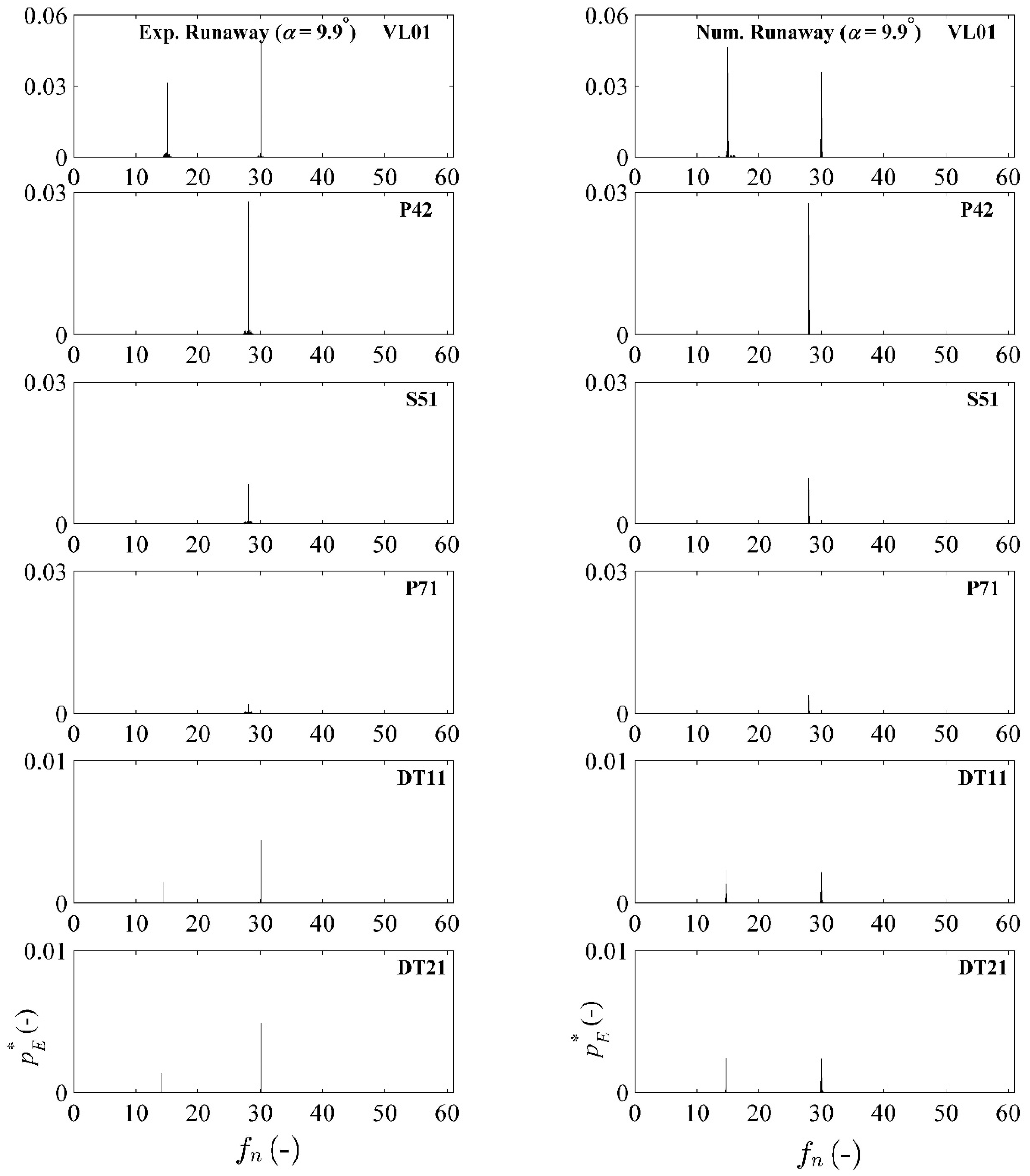
A power spectral density (PSD) analysis of the pressure-time signals was performed for all of the points at the runaway conditions. Figure 13 shows the PSD analysis of the pressure-time signals that were obtained for the runaway operating condition at an angular position of the guide vanes of 9.9°. The experimental and numerical frequency spectra at the pressure measurement at locations VL01, P42, S51, P71, DT11 and DT21 are compared in the figure. The pressure-time data of the measurement were processed through a designed filter in MATLAB to enhance the visualization of the investigated frequencies and the corresponding amplitudes. The frequencies that were not related to the flow were filtered out, i.e., noise, vibrations and frequencies of the electrical power (50 and 100 Hz). The MATLAB designed “bandpass” and “band stop” filter were used to filter out the frequencies [28].

The turbine consisted of 28 guide vanes and 30 blades, including 15 splitters. The obtained frequencies were normalized by the angular speed of the runner (n_R = 8.74 Hz). Therefore, a dimensionless frequency (f_n) of 15 with its harmonics was used to represent the blade passing frequency in the stationary domains, and a dimensionless frequency of 28 with its harmonics was used to represent the guide vanes’ passing frequency in the rotating domain. The amplitudes of these frequencies were normalized using Equation (5). Thus, the dimensionless frequency and amplitude are discussed in this section.

In the vaneless space (VL01), two frequencies of 15 and 30 were observed with high amplitude pressure fluctuations. The frequency of 15 corresponded to the sub-harmonic of the blade passing frequency. The blade passing frequency had a maximum amplitude of 0.05. These two frequencies were also obtained by analyzing the numerical pressure-time data at VL01. However, the frequencies had different amplitudes. The amplitude for the blade passing frequency was approximately 29% lower than the experimental value.

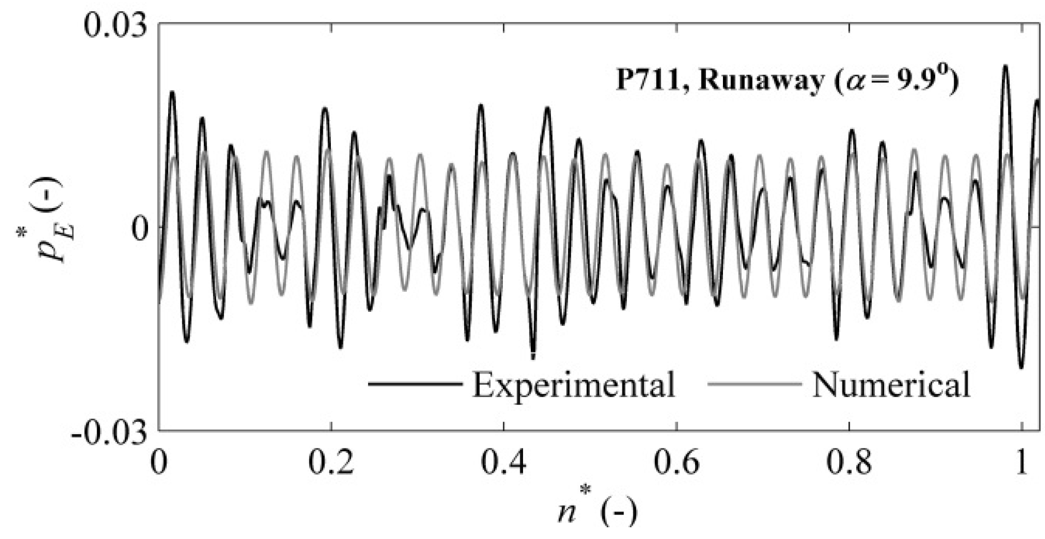
A spectral analysis of the numerical and experiment pressure-time signals acquired from the runner blade sensors at P42, S52 and P71 yielded a guide vane passing frequency of 28 at the maximum amplitude. At P42, the numerical amplitude of the guide vane passing frequency was 3% higher than the corresponding experimental value (0.024). For S51 and P71, the numerical amplitudes were 2 and 5% higher, respectively, than the experimental values. No other frequency with such a high amplitude was observed in the runner. However, the amplitude of the guide vane passing frequency at the runaway condition was more than two-times the amplitude at the BEP.

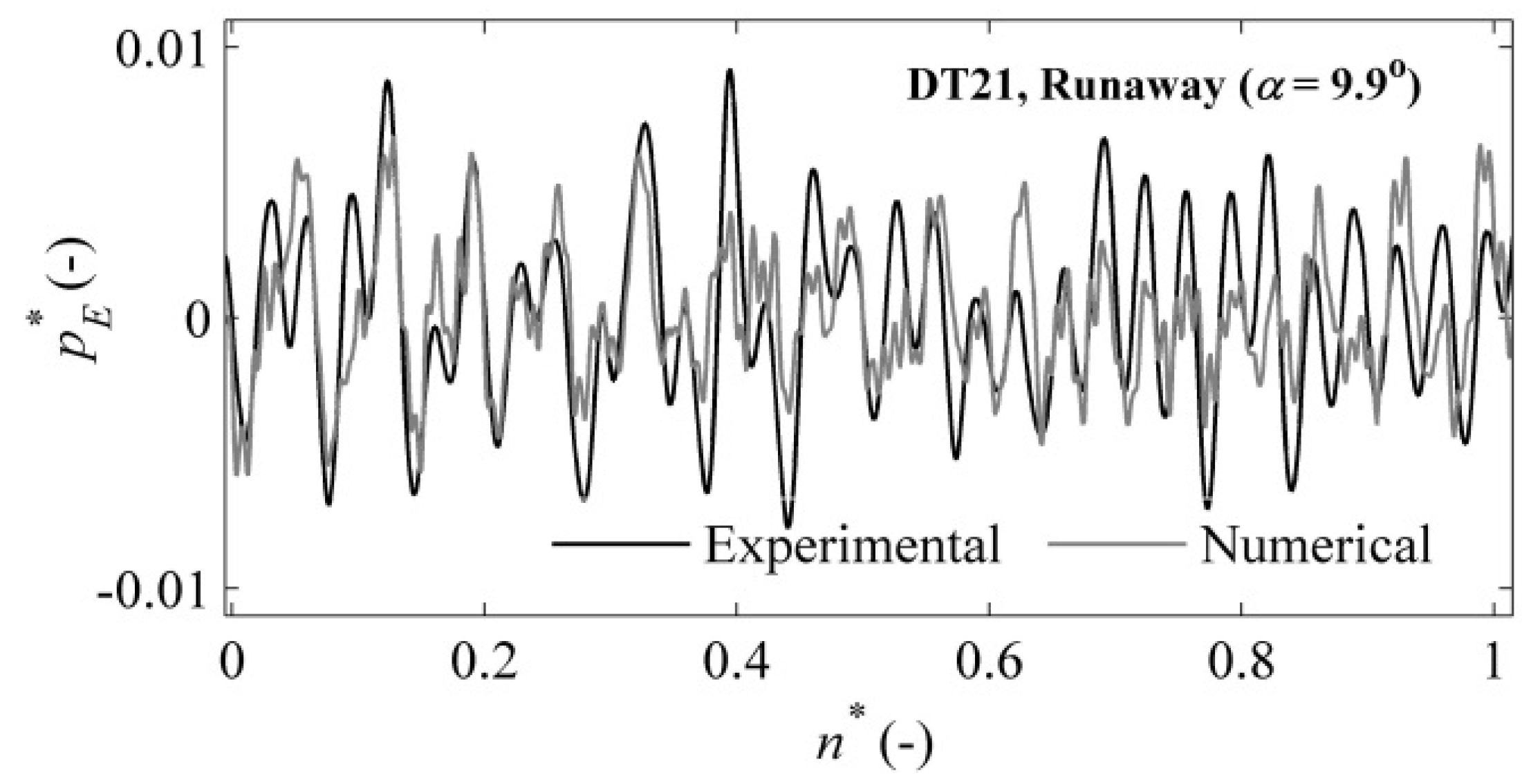
At DT11 and DT21 in the draft tube, a high-amplitude (0.002) blade passing frequency (f_n = 15) was observed numerically. The amplitude of the numerical pressure-time data was approximately 12% higher than the corresponding experimental value. Another dimensionless frequency of 30, the first harmonic, was observed for both numerical and experimental data. No other frequency related to the vortex rope or axial pressure pulsations was observed in the spectral analysis of the data from DT11 and DT21. A vortex rope may not have developed under these conditions because the discharge to the runner was extremely low, and the runner was rotating at the runaway speed, which was more than 150% of the synchronous speed.

6. Unsteady Flow in the Runner

A small difference between the experimental and numerical results provided us with the confidence for further investigation into the complex flow passage of the runner. The turbine runner includes 15 splitters and 15 blades. The blades are highly twisted, which make a turn of 178° from the leading edge to the trailing edge. The length of the splitter is half of the blade. The analysis of the flow field in the runner showed that there was a swirling flow in the blade passages at the runaway operating conditions. 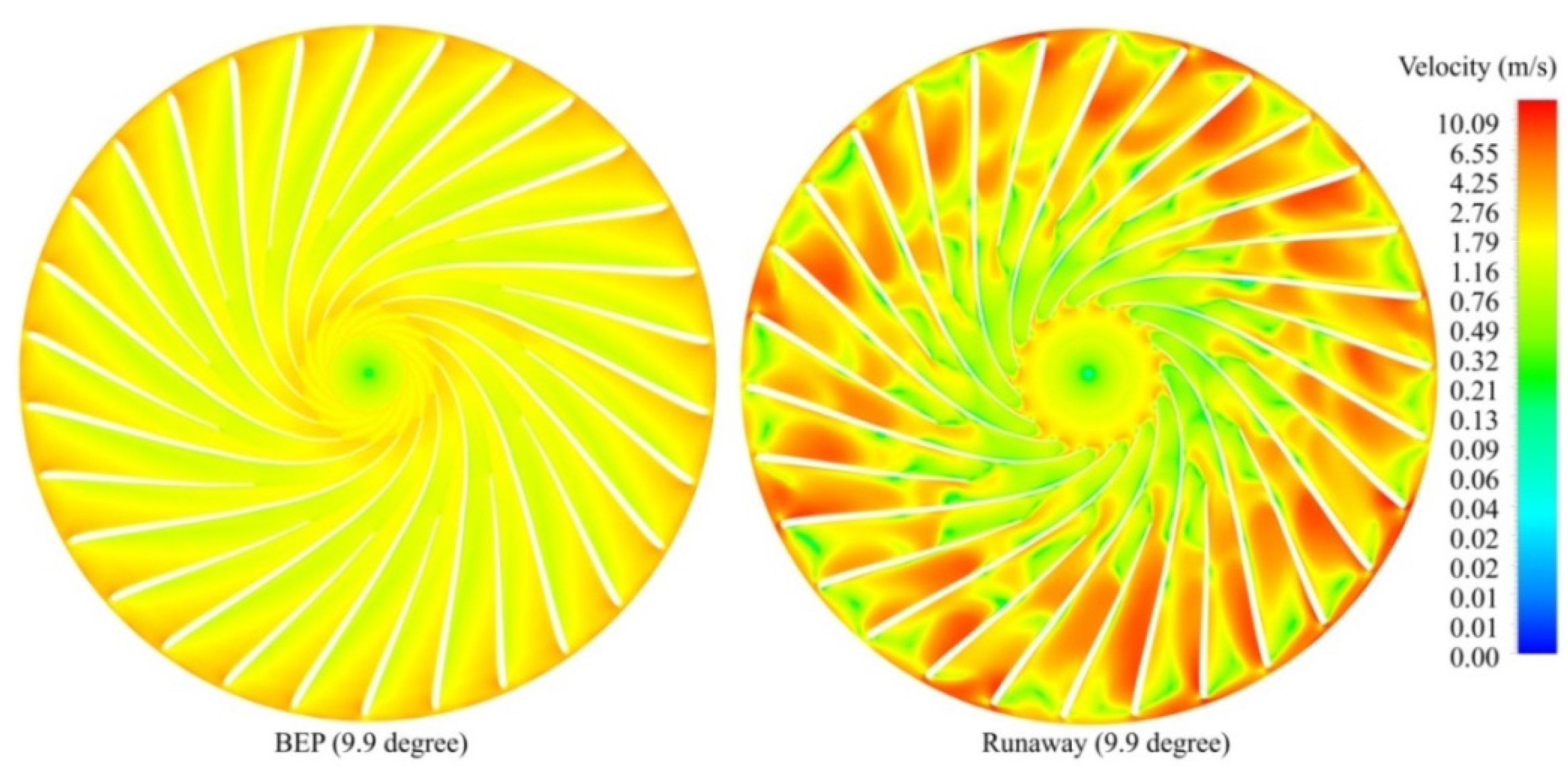Figure 14 shows the velocity distribution contours near the surface of the runner crown at the BEP and the runaway condition at a guide vane angular position of 9.9°. A new plane was created 5 mm below the crown to extract the velocity distribution near the crown. The flow field is shown in the rotating frame of reference. The velocity contours are shown at the instant after 10 revolutions of the runner, i.e., t = 1.81 and 1.14 s, for the BEP and the runaway condition, respectively. The same mesh was used for the simulation at both operating conditions. At the BEP, a uniform velocity distribution was obtained for the blade passages, and the flow was almost streamlined, whereas a non-uniform flow field was observed at the runaway condition. The flow field in the blade passages evolved with time and the angular movement of the runner.

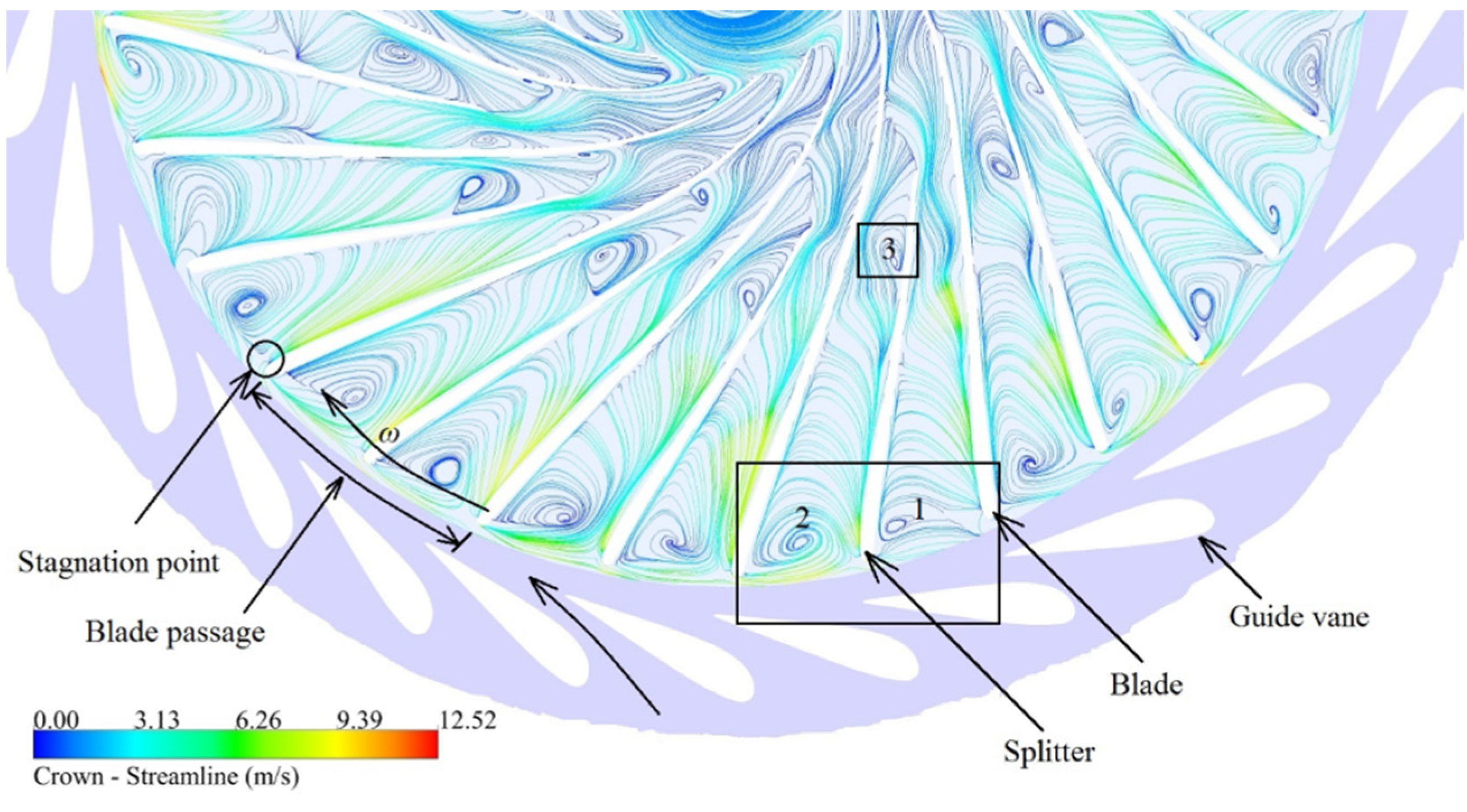
In the following, a blade passage starts from the pressure side of a blade and ends at the suction side of the opposite blade. Each passage makes an angle of 24° (=360°/15 passages), from the pressure side of a blade to the suction side of a splitter (i.e., 12°) and the pressure side of the splitter to the suction side of the opposite blade (i.e., 12°). During the runaway operating condition (α = 9.9°), a high relative velocity (~10 m·s⁻¹) was obtained near the blade suction side from the runner upstream to the downstream. In the runner, the area of the blade passage decreased from the inlet to the outlet, and the fluid velocity also appeared to simultaneously decrease along the passage. The large variation in the relative velocity in the passage could have produced an unsteady flow. The flow appeared to accelerate near the suction side and decelerate at the pressure side. The runner rotated under a no load condition at a significantly high speed and a low discharge.

Figure 15 shows the velocity streamlines on the runner crown surface at the same instant (i.e., t = 1.14 s) at the runaway operating condition (α = 9.9°). Three regions with a vortical flow can be observed. Two regions were at the inlet of the blade passage and are marked as “1” and “2”; a third region marked as “3” was located between the splitter suction side and the blade pressure side, near the splitter trailing edge. The rotating direction of the vortical flow in Regions 1 and 2 was opposite the direction of the runner rotation, whereas the direction of the vortical flow in Region 3 was the same as the runner rotation. Similar vortical regions were observed for all of the blade passages of the runner.

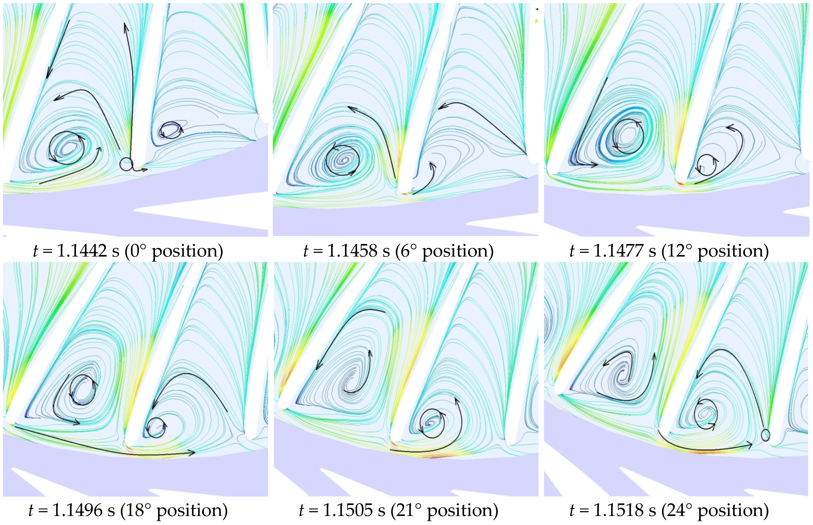
Figure 16 shows the instantaneous variation in the flow field in the rotating frame that is marked by a rectangle in Figure 16. The velocity streamlines on the runner crown are shown for a total time of 0.0076 s (i.e., a 24° angular movement of the runner), and the color scale is the same as that shown in Figure 16. The vortical region may have developed based on the angular position of the blade passage. The vortical region started to form when a blade was positioned in front of a guide vane trailing edge. At an angular position of 0°, Vortical Region 1 began to form, and Vortical Region 2 had already developed because of the previous angular movement. At the splitter leading edge, i.e., the stagnation point, the flow separated into three directions (see the blade passage at t = 1.1442 s): (i) a portion of the flow accelerated toward the blade channel; (ii) a portion of the flow traveled toward Vortical Region 2; and (iii) a portion of the flow traveled toward the vaneless space in the direction of the runner rotation. At an angular position of 12°, Region 1 evolved further, and the flow rotated about a local axis in the counter clockwise direction. At an angular position of 24°, Region 1 became larger. Thus, the vortical flow developed with time up to an angular position of 74°. The cycle was observed and repeated for each angular movement of 74° of the runner. A similar phenomenon was observed for Vortical Region 2.

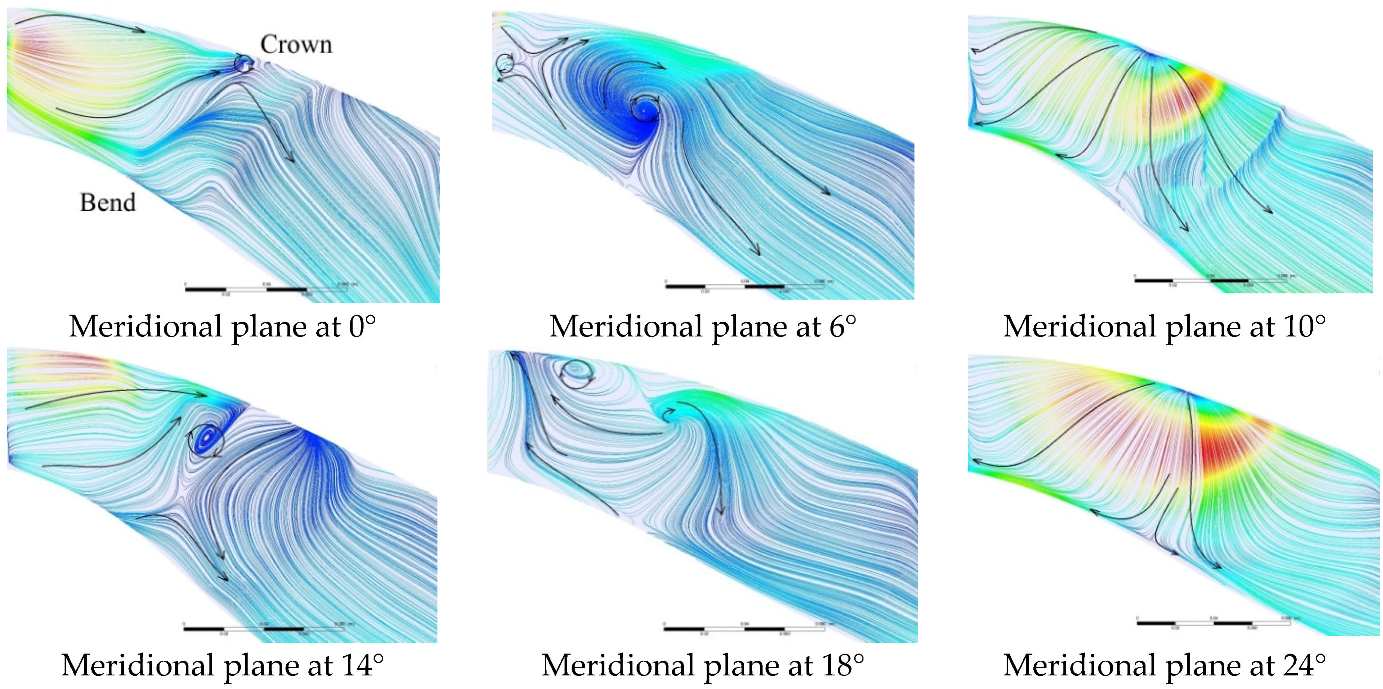
Figure 17 shows the streamlines in a meridional plane for the same blade passage at an instant in time (t = 1.1442 s). A total of six sections are shown ranging from 0 to 24°. At the meridional plane at 0°, i.e., the suction side of the blade, the flow generally accelerated downstream, and a small vortical region was observed near the crown. At the meridional plane at 6°, i.e., the middle of the blade channel, the development of a large vortical region that rotated in the clockwise direction was clearly observed. The flow at the crown side accelerated more than at the band side, which may have created a large pressure difference in the channel, causing the flow to recirculate. The entire vortical flow region was pushed to the down side of the passage by the angular motion of the runner. At the meridional plane at 10°, i.e., the pressure side of the splitter, the flow accelerated from the crown to the band side. At the meridional plane at 14°, i.e., the suction side of the splitter, the flow field was almost similar to that observed at the 0° plane. At the meridional plane at 18°, i.e., the middle of the blade channel, reversed flow was observed. A portion of the flow accelerated to the down side, while another portion of the flow flowed back to the up side, and a swirling region developed near the crown. The swirling flow rotated in a clockwise direction. At the meridional plane of 24°, i.e., the pressure side of the next blade, the flow was fairly similar to that observed at the 10° plane. In summary, a strong secondary flow was created in the blade channels, producing considerable losses and pressure fluctuations.

Unsteady flow in the blade passage was observed at the runaway operating condition. The flow field may have been primarily driven by the pressure difference that developed in the blade channel along the passage length from the inlet to the outlet. On the pressure side surfaces, the flow generally traveled from the band to the crown and then accelerated to the down side of the channel. On the suction side, the flow accelerated from the crown to the band side and divided into two directions, the up and down sides of the channel. The strongest swirling flow was observed in the middle of the channel and rotated in the clockwise direction. The direction of rotation was driven by the pressure difference between the crown and band, because the flow accelerated more at the crown side than the band side.

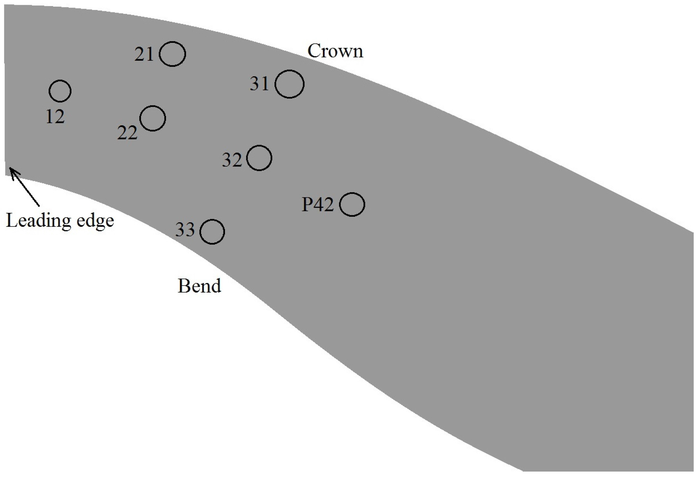
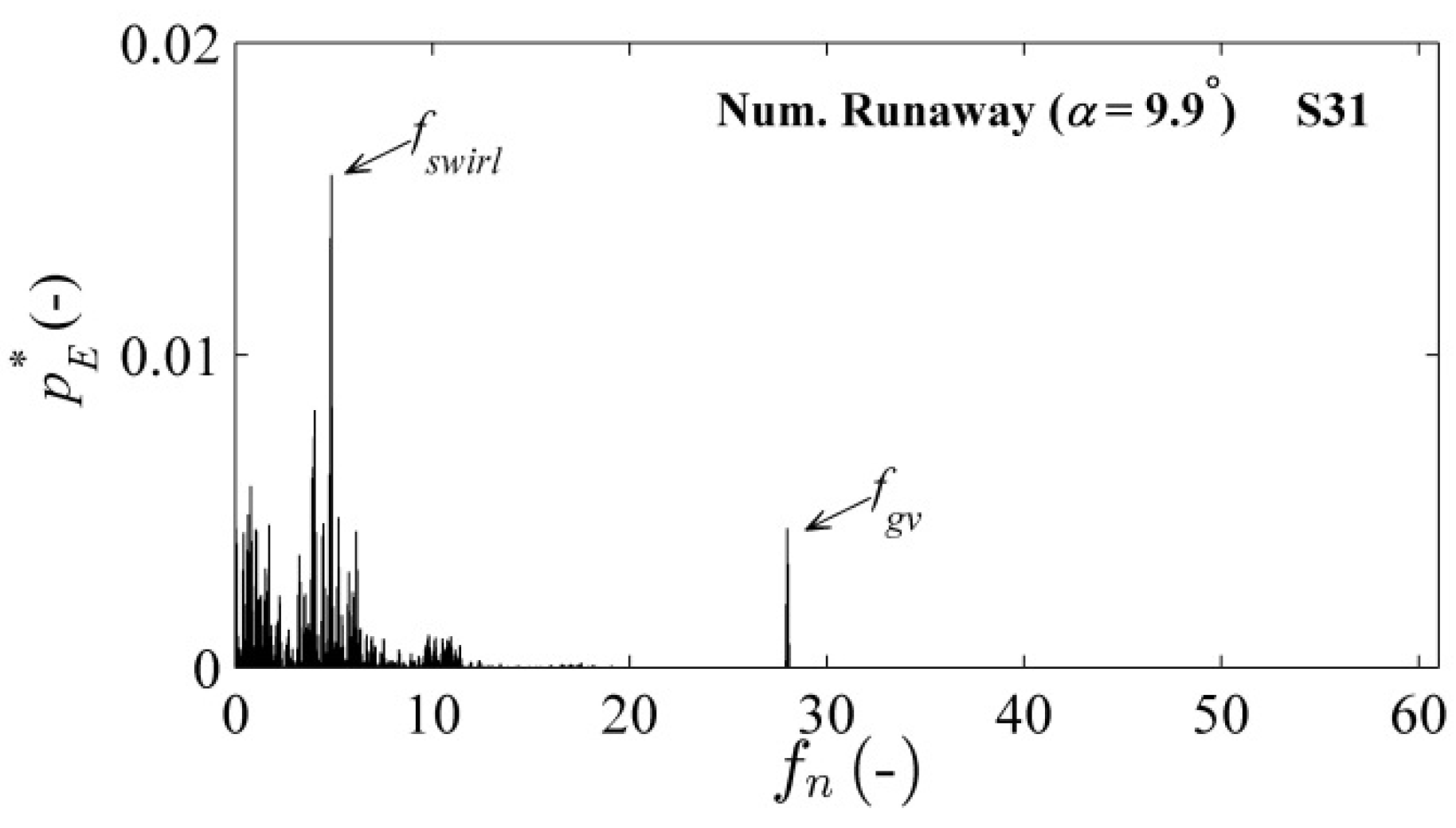
A grid of numerical points was created on the meridional plane at the blade pressure and the suction sides to monitor the pressure variation related to the angular motion of the runner. Some of the grid points are shown in Figure 18. A PSD analysis was performed on all of the numerical pressure-time signals obtained from the grid points. A dimensionless frequency (f_swirl) of 4.8 (42.24 Hz) was obtained at all of the locations, and the maximum amplitude was observed at two locations, S31 and P32. Figure 19 shows the spectral analysis of the pressure-time signals at S31. The dimensionless numerical amplitude of the frequency f_swirl was 0.015, which corresponded to an absolute value of 1.8 kPa. The dimensionless frequency of 4.8 corresponded to the angular movement of the runner of 74.5°, which matched the angle of the maximum vorticity, as was discussed for the angular movement of the blade passage. Figure 17 shows the strong effect of the vortical flow at S31 and P32 at the instantaneous angular positions of 10 and 18°, respectively.

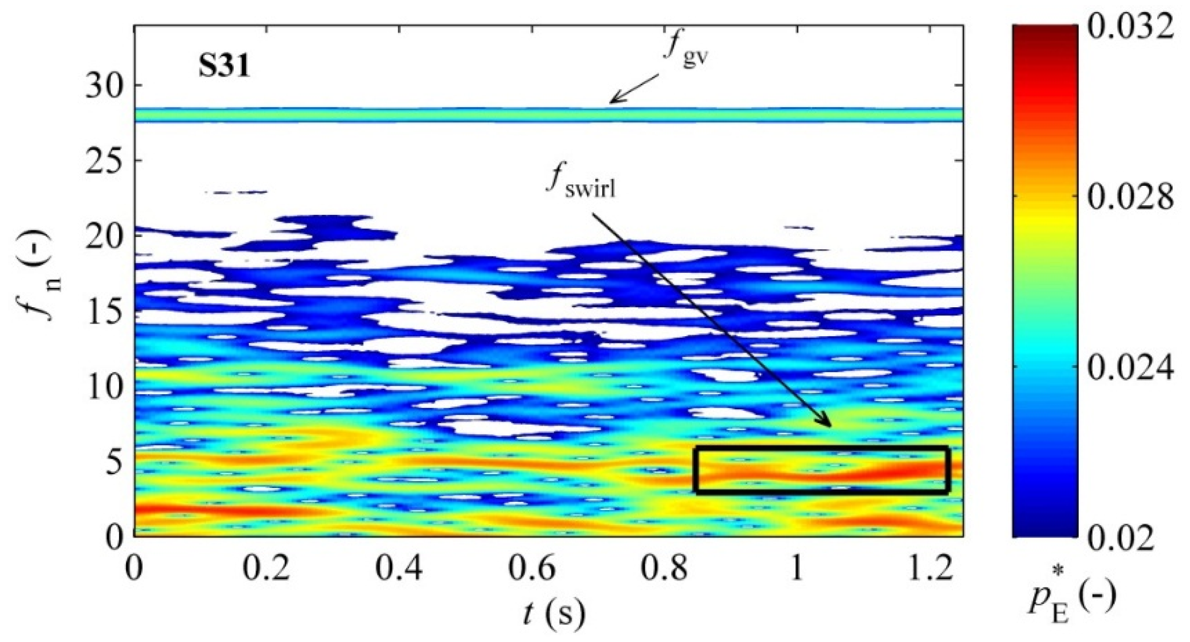
A short-time Fourier transform (STFT) analysis was also performed on all of the points around P32 and S32 to investigate the time-dependent variation of the dimensionless frequency of 4.8. The maximum amplitude of this frequency was observed at S31 (see Figure 20). The amplitude varied with time/the angular movement of the runner. Surprisingly, this amplitude was higher than that of the guide vane passing frequency (f_gv), indicating the strong effect of the secondary swirling flow in the runner at the runaway operating conditions.

7. Conclusions

A runaway operating condition is one of the most damaging conditions for hydraulic turbines, because the associated pressure fluctuations have extremely high amplitudes, and the runner operates at a very high speed. The unsteady pressure loading in the turbine during the runaway operating condition more than doubles relative to normal operating conditions. Consequently, the runner vibrations are high because the runner rotates at a high speed with no load. The unsteady pressure loading at different locations of the turbine was investigated numerically and validated. Three operating points of the runaway condition over the turbine operating range were investigated.

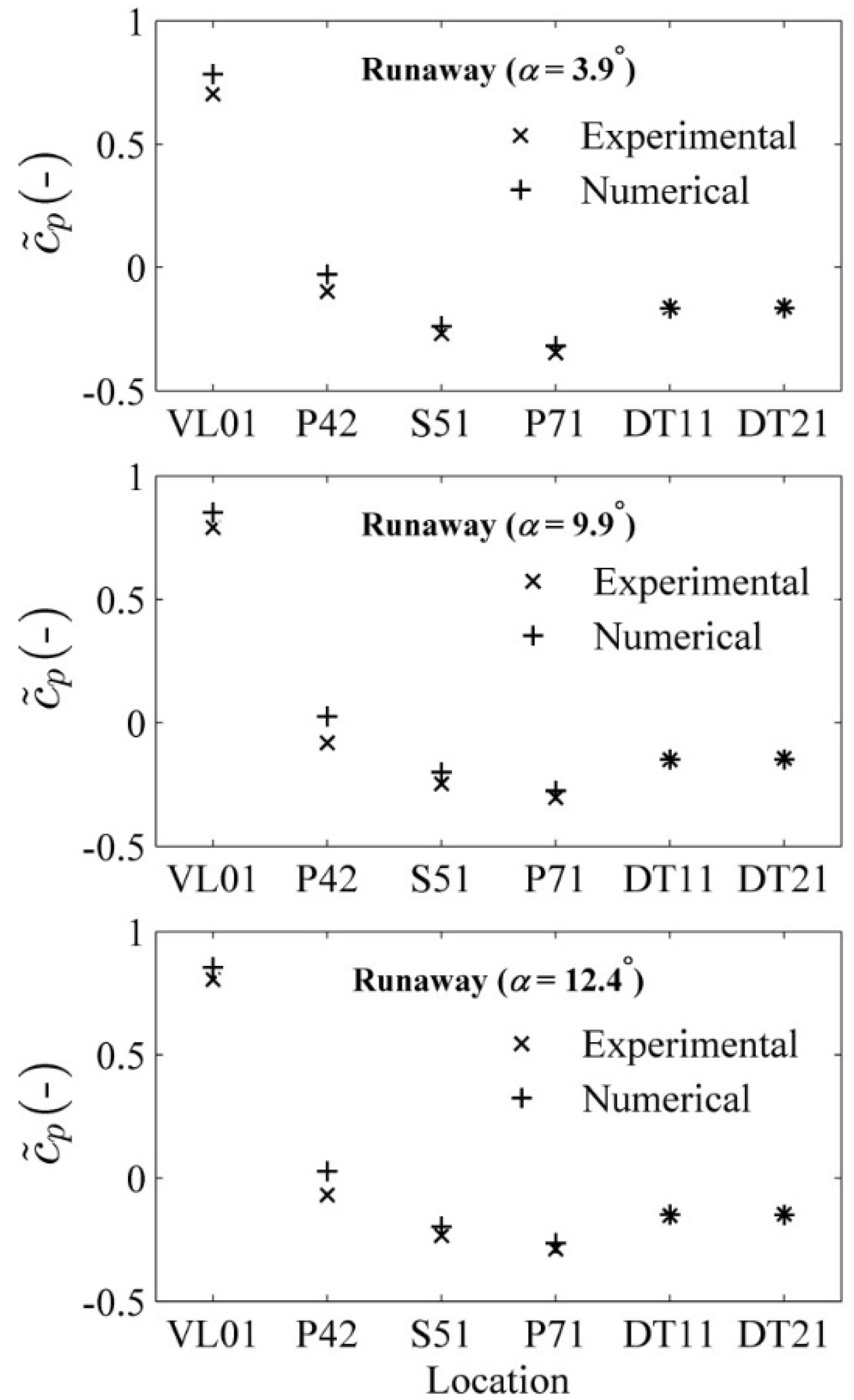
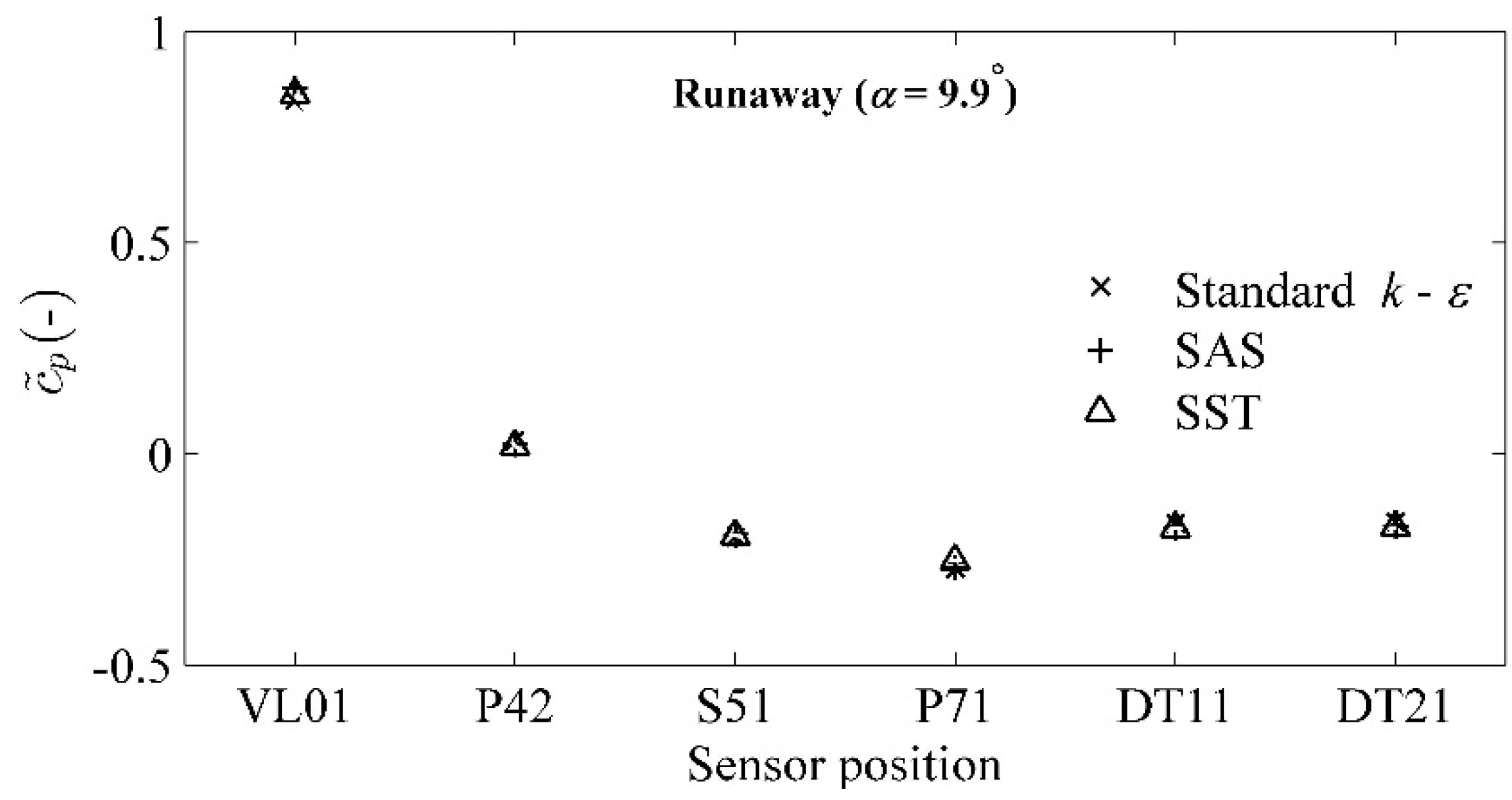
Similar differences between the experimental and numerical dimensionless pressure coefficients were obtained at the investigated points of the runaway condition. A maximum difference of 12.8% between the experimental and numerical results was observed in the runner. This result could be attributed to the under-prediction of the losses from flow separation in the runner. The deviation may be attributed to the variation in capturing the flow unsteadiness (a rotating stall-type condition) due to the large grid size at some locations of the turbine. However, the difference between the experimental and numerical values was within the band of numerical uncertainties that was estimated in the mesh performance analysis. In the draft tube, a moderate pressure difference of 2.1% was observed. Moderate differences between the time-averaged experimental and numerical pressure values were found for the vaneless space and the runner. A PSD analysis of the time-averaged pressure signal for the vaneless space yielded an extremely high amplitude at the runaway condition, which was 2.8-times the amplitude observed at the BEP.

Three turbulence models, standard k-ε, SST k-ω and SAS-SST, were used for the numerical simulations at the runaway condition. The SAS-SST model was used for detailed analysis in the turbine as this hybrid model has the advantage of capturing unsteady flow features over standard k-ε and SST k-ω models. A detailed analysis of the flow field in the runner showed a generally unstable and unsteady vortical flow in the blade passages during the runaway operating condition. The vortical flow was observed at three locations for each blade passage. At two of the locations, the flow rotated in a counter clockwise direction, and at one location, the flow rotated in the same direction as the runner, i.e., clockwise. The frequency of the vortical flow was 4.8·n_R, which corresponded to an angular movement of the runner of 74.5° at the runaway speed (n_R = 8.74 s⁻¹). A PSD analysis of the numerical pressure signal at these locations yielded similar frequencies, indicating the presence of swirling flow with an absolute amplitude of 1.8 kPa. The amplitude was more than twice that of the guide vanes’ passing frequency in the swirling flow regions. Thus, the unsteady flow that resulted from the rotating swirl at a frequency of 4.8·n_R was observed at the runaway operating conditions where the pressure and velocity distribution was non-uniform, as was observed under normal operating conditions. This behavior may have been one of the causes of the high-amplitude unsteady pressure loading. The unsteady pressure loading induce fatigue to the blades, which affects the operating life of the turbine runner, specifically when the transition from total load rejection to the runaway condition takes place.

8. Future Work

A detailed study of the high head model Francis turbine was conducted. Both experimental and numerical studies showed the strong effect of rotor stator interaction in the turbine at runaway speed. The numerical study also indicated the rotating stall-type condition in the runner. Such challenging flow conditions may cause significant damage to the turbine runner and induce fatigue damage. In order to investigate in detail, further investigations and blade optimizations are needed. The present investigations do not account for the cavitation condition. Therefore, future measurements would include cavitation and measurements at significantly affected areas in the runner, as observed in Figure 16 and Figure 17. By taking advantage of the improvement in numerical techniques and the implementation in ANSYS CFX, automatic optimization would be possible using this data. The blade profile can be improved further. The improved blade profile would benefit the stable operation of the turbines.

References

1. Sawin, J.L.; Sverrisson, F.; Rickerson, W. Renewables 2015 Global Status Report; Mastny, L., Ed.; REN21: Paris, France, 2015; p. 251. [Google Scholar]
2. Trivedi, C.; Cervantes, M.; Gandhi, B.; Dahlhaug, O. Transient pressure measurements on a high head model Francis turbine during emergency shutdown, total load rejection, and runaway. ASME J. Fluids Eng. 2014, 136. [Google Scholar] [CrossRef]
3. Zeng, W.; Yang, J.; Guo, W. Runaway Instability of Pump-Turbines in S-Shaped Regions Considering Water Compressibility. J. Fluids Eng. 2015, 137. [Google Scholar] [CrossRef]
4. Trivedi, C.; Gandhi, B.; Cervantes, M. Effect of transients on Francis turbine runner life: A review. J. Hydraul. Res. 2013, 51, 121–132. [Google Scholar] [CrossRef]
5. Nicolet, C. Hydroacoustic Modelling and Numerical Simulation of Unsteady Operation of Hydroelectric Systems; Ecole Polytechnique Federale de Lausanne: Lausanne, Switzerland, 2007; p. 334. [Google Scholar]
6. Liu, S.; Zhou, D.; Liu, D.; Wu, Y.; Nishi, M. Runaway transient simulation of a model Kaplan turbine. IOP 2010, 12. [Google Scholar] [CrossRef]
7. Brekke, H. Performance and safety of hydraulic turbines. IOP 2010, 12. [Google Scholar] [CrossRef]
8. Dörfler, P.; Sick, M.; Coutu, A. Flow-Induced Pulsation and Vibration in Hydroelectric Machinery, 1st ed.; Springer-Verlag: London, UK, 2013; p. 242. [Google Scholar]
9. Kolšek, T.; Duhovnik, J.; Bergant, A. Simulation of unsteady flow and runner rotation during shut-down of an axial water turbine. J. Hydraul. Res. 2006, 44, 129–137. [Google Scholar] [CrossRef]
10. Gagnon, M.; Léonard, F. Transient Response and Life Assessment: Case Studies on the Load Rejection of two hydroelectric turbines. In Proceedings of the International Conference Surveillance 7, Chartres, France, 29–30 October 2013.
11. Trivedi, C.; Cervantes, M.; Dahlhaug, O.; Gandhi, B. Experimental investigation of a high head Francis turbine during spin-no-load operation. ASME J. Fluids Eng. 2015, 137. [Google Scholar] [CrossRef]
12. Trivedi, C.; Cervantes, M.; Gandhi, B.; Dahlhaug, O. Experimental investigations of transient pressure variations in a high head model Francis turbine during start-up and shutdown. J. Hydrodyn. Ser. B 2014, 26, 277–290. [Google Scholar] [CrossRef]
13. Fortin, M.; Houde, S.; Deschênes, C. Validation of simulation strategies for the flow in a model propeller turbine during a runaway event. IOP Conf. Ser. Earth Environ. Sci. 2014, 22. [Google Scholar] [CrossRef]
14. Hosseinimanesh, H.; Vu, T.C.; Devals, C.; Nennemann, B.; Guibault, F. A steady-state simulation methodology for predicting runaway speed in Francis turbines. IOP Conf. Ser. Earth Environ. Sci. 2014, 22. [Google Scholar] [CrossRef]
15. Trivedi, C.; Cervantes, M.; Gandhi, B.; Dahlhaug, O. Pressure measurements on a high-head Francis turbine during load acceptance and rejection. J. Hydraul. Res. 2014, 52, 283–297. [Google Scholar]
16. Trivedi, C.; Gandhi, B.; Cervantes, M.; Dahlhaug, O. Experimental investigations of a model Francis turbine during shutdown at synchronous speed. Renew. Energy 2015, 83, 828–836. [Google Scholar] [CrossRef]
17. Widmer, C.; Staubli, T.; Ledergerber, N. Unstable characteristics and rotating stall in turbine brake operation of pump-turbines. ASME J. Fluids Eng. 2011, 133. [Google Scholar] [CrossRef]
18. Bjorkvoll, T.; Bakken, B.H. Calculating the start-up costs of hydropower generators. In Proceedings of the 14th Power Systems Computation Conference (PSCC 2002 SEVILLE), Sevilla, Spain, 24–28 June 2002.
19. Coutu, A.; Lauzon, J.; Monette, C.; Nennemann, B.; Huang, X. Francis runner: Cost of operation, presentation. In Proceedings of the 5th IAHR International Workshop on Cavitation and Dynamic Problems in Hydraulic Machinery, Lausanne, Switzerland, 8–11 September 2013.
20. Nilsson, O.; Sjelvgren, D. Hydro unit start-up costs and their impact on the short term scheduling strategies of swedish power producers. IEEE Trans. Power Syst. 1997, 12. [Google Scholar] [CrossRef]
21. International Electrotechnical Commission (IEC). Hydraulic turbines, storage pumps and pump-turbines—Model acceptance tests. In Proceedings of the International Electrotechnical Commission: 3, Geneva, Switzerland, 1999; p. 578.
22. Hasmatuchi, V. Hydrodynamics of a Pump-Turbine Operating at Off-Design Conditions in Generating Mode, in A la Faculte Sciences et Techniques de L’ingenieur; École Polytechnique Fédérale de Lausanne: Lausanne, Switzerland, 2012; p. 188. [Google Scholar]
23. Celik, I.B.; Ghia, U.; Roache, P.J.; Freitas, C.J. Procedure for estimation and reporting of uncertainty due to discretization in CFD applications. ASME J. Fluids Eng. 2008, 130. [Google Scholar] [CrossRef]
24. ANSYS, version 16.0; Theory and Modelling Guide; ANSYS Inc.: Canonsburg, PA, USA, 2015.
25. Menter, F.R.; Egorov, Y. SAS Turbulence Modelling of Technical Flows. In Direct and Large-Eddy Simulation VI; Lamballais, E., Friedrich, R., Geurts, B.J., Métais, O., Eds.; Springer: Dordrecht, The Netherlands, 2006; pp. 687–694. [Google Scholar]
26. Egorov, Y.; Menter, F. Development and Application of SST-SAS Turbulence Model in the DESIDER Project, in Advances in Hybrid RANS-LES Modelling; Peng, S.-H., Haase, W., Eds.; Springer: Berlin, Germany, 2008; pp. 261–270. [Google Scholar]
27. Nicolle, J.; Cupillard, S. Prediction of dynamic blade loading of the Francis-99 turbine. J. Phys. Conf. Ser. 2015, 579. [Google Scholar] [CrossRef]
28. Dolecek, G.J. Random Signals and Processes Primer with Matlab; Springer: New York, NY, USA, 2013; p. 530. [Google Scholar]
Figure 1. Locations of the six sensors for pressure measurements at runaway operating condition: VL01, vaneless space; P42, blade pressure side; P71, blade pressure side trailing edge; S51, blade suction side; DT11 and DT21, draft tube cone; GV, guide vane; Interface-I and Interface-II correspond to the inlet and outlet of the rotating domain, i.e., the runner.
Energies 09 00149 g001
Figure 2. Computational domain for the Francis turbine: Interface-I, connecting the distributor and runner; Interface-II, connecting the runner and draft tube. The interfaces are located at the runner inlet and the runner outlet locations. Exact interface locations can be seen in Figure 1.
Energies 09 00149 g002
Figure 3. Hexahedral mesh for the distributor and runner of the Francis turbine.
Energies 09 00149 g003
Figure 4. Comparison between experimental and numerical hydraulic efficiencies at five operating points, showing the performance of the numerical model at different operating conditions for the model Francis turbine; Q = 0.2 m3·s−1 is discharge at BEP. NUM corresponds to numerical data.
Energies 09 00149 g004
Figure 5. Comparison between the experimental and numerical values of pressure coefficient at different locations in the turbine, showing the runaway conditions at three angular positions of the guide vanes: 3.9, 9.9 and 12.4°.
Energies 09 00149 g005
Figure 6. Comparison of the pressure coefficient computed using three turbulence models, standard k-ε, SAS (scale-adaptive simulation) and SST (shear stress transport), at different locations in the turbine, showing the runaway conditions at 9.9° angular positions of the guide vanes.
Energies 09 00149 g006
Figure 7. Contours of the pressure coefficient on the blade pressure side and suction side at the runaway (α = 12.4°) operating condition.
Energies 09 00149 g007
Figure 8. Instantaneous pressure fluctuations in the vaneless space (VL01) at BEP and runaway (α = 9.9°) operating conditions for one second; pressure fluctuations occur at the blade passing frequency in the vaneless space, which is induced by the rotor stator interaction.
Energies 09 00149 g008
Figure 9. Instantaneous pressure fluctuations in the vaneless space (VL01) over a complete rotation of the runner at the runaway point α = 9.9°; fluctuations occur at a rotor stator interaction and blade passing frequency of 262.2 Hz and its harmonic of 131.1 Hz.
Energies 09 00149 g009
Figure 10. Instantaneous pressure fluctuations at the blade pressure side (P42) over a complete rotation of the runner for the runaway operating point α = 9.9°; the fluctuations correspond to the rotor stator interaction and a guide vane passing frequency of 244.7 Hz.
Energies 09 00149 g010
Figure 11. Instantaneous pressure fluctuations at the blade trailing edge (P71) over a complete rotation of the runner for the runaway operating point α = 9.9°; fluctuations occur at a rotor stator interaction and guide vane passing frequency of 244.7 Hz.
Energies 09 00149 g011
Figure 12. Instantaneous pressure fluctuations in the draft tube cone (DT21) over a complete rotation of the runner for the runaway operating point α = 9.9°; fluctuations occur at a rotor stator interaction and blade passing frequency of 262.2 Hz.
Energies 09 00149 g012
Figure 13. Frequency spectrum of experimental and numerical pressure-time signals in the vaneless space (VL01), runner (P42, S51 and P71) and draft tube (DT11 and DT21); the frequencies shown are normalized by a runner angular speed of 8.74 Hz; the dimensionless frequencies of 30 and 28 correspond to the blade passing and the guide vane passing frequencies, respectively.
Energies 09 00149 g013
Figure 14. Contours of the velocity distribution near the surface of the runner crown at BEP and runaway (α = 9.9°) operating conditions; the contours are in a rotating frame of reference, and a logarithmic scale is shown.
Energies 09 00149 g014
Figure 15. Flow streamlines near the crown surface at the runaway operating condition (α = 9.9), where the velocity distribution shown is in the rotating frame of reference; ω corresponds to the direction of the runner angular movement, i.e., clockwise; Points 1, 2 and 3 show the vortical flow regions in a blade passage; the runner includes 15 blades and 15 splitters; n = 8.74 Hz, Q = 0.08 m3·s−1, H = 12.27 m.
Energies 09 00149 g015
Figure 16. Time-dependent variation in the flow field on the runner surface crown during an angular movement of the runner of 24° at the runaway speed (α = 9.9°); this zoom of the rectangle marked in Figure 16 for the passage includes the blade pressure side, the splitter suction side, the splitter pressure side and the blade suction side; the streamlined color scale is similar to Figure 15 in the rotating frame of reference.
Energies 09 00149 g016
Figure 17. Flow field for the meridional planes of the runner at the instant t = 1.1442 s; the planes at 0, 10, 14 and 24° indicate the suction side of the blade, the pressure side of the splitter, the suction side of the splitter and the pressure side of the next blade, respectively; the planes at 6 and 18° indicate the middle of the two blade channels; bold arrows indicate the flow direction from/to the swirling regions; the color scales of the streamlines are similar to those used in Figure 15 in the rotating frame of reference.
Energies 09 00149 g017
Figure 18. Meridional plane showing numerical monitoring points used to obtain pressure-time data from vortical flow regions.
Energies 09 00149 g018
Figure 19. PSD analysis of the numerical point S32 on the blade suction side; fgv corresponds to the frequency of guide vane passing.
Energies 09 00149 g019
Figure 20. Time-dependent variation in the swirl frequency 4.8·nR at S31 at the runaway operating condition (α = 9.9°); fgv denotes the guide vane passing frequency (28), fswirl denotes the swirl frequency at S31.
Energies 09 00149 g020