Robust Optimization-Based Scheduling of Multi-Microgrids Considering Uncertainties

Abstract

Scheduling of multi-microgrids (MMGs) is one of the important tasks in MMG operation and it faces new challenges as the integration of demand response (DR) programs and renewable generation (wind and solar) sources increases. In order to address these challenges, robust optimization (RO)-based scheduling has been proposed in this paper considering uncertainties in both renewable energy sources and forecasted electric loads. Initially, a cost minimization deterministic model has been formulated for the MMG system. Then, it has been transformed to a min-max robust counterpart and finally, a traceable robust counterpart has been formulated using linear duality theory and Karush–Kuhn–Tucker (KKT) optimality conditions. The developed model provides immunity against the worst-case realization within the provided uncertainty bounds. Budget of uncertainty has been used to develop a trade-off between the conservatism of solution and probability of unfeasible solution. The effect of uncertainty gaps on internal and external trading, operation cost, unit commitment of dispatchable generators, and state of charge (SOC) of battery energy storage systems (BESSs) have also been analyzed in both grid-connected and islanded modes. Simulations results have proved the robustness of proposed strategy.

1. Introduction

A typical microgrid (MG) comprises of various distributed generations (DGs), energy storage systems (ESSs), and loads and it can operate in both grid-connected and islanded modes [1]. Microgrids have the ability to sustain penetration of renewable generations (RGs), plug-in hybrid vehicles, and energy storage systems. In addition, MGs can support the main distribution system by supplying/absorbing power [1]. Microgrids also have an enormous potential to provide service reliability, reduce emissions, and improve power quality for the end-use customers through the utilization of DGs, ESSs, and DR programs.

In order to achieve the fore-mentioned benefits of MGs, penetration of renewable generation resources and DR programs has significantly increased in the recent years. This enhanced penetration has imposed new challenges to the scheduling of microgrids [2]. Various forecasting techniques are used for forecasting the electric load demands [3], demand response (DR) [4], and RGs [5] (wind and solar generations) considering various environmental factors like wind speed [6], solar irradiance [7], and weather intelligence and history data [8]. However, due to various unpredictable natural phenomena, these forecasted values are not accurate. Owing to the significance of uncertainties associated with power generation of RGs and forecasted load demands in microgrids, uncertainty management has become an active research area in scheduling of MG systems in the recent years. Conventionally spinning and non-spinning reserves have been used for managing the uncertainties associated with the distribution systems [9]. However, in the past few years, various novel techniques have been introduced by researchers for managing the uncertainties in microgrids. Sensitivity analysis [10], fuzzy logic-based optimization [11], stochastic optimization techniques [12], and robust optimization [13,14,15,16] are among the noticeable techniques available in the literature for uncertainty management in scheduling of active distribution systems and microgrids. The drawbacks associated with each of the uncertainty management technique are summarized in the following paragraphs.

The discrepancy between the forecasted values and realization has been relatively small in the conventional distribution systems [9]. Therefore, reserves have been commonly used for catering these minor discrepancies. However, in multi-microgrid systems this solution is not feasible. Sensitivity analysis being a post-operation analysis technique is not capable of providing any immunity against the uncertainties. Determination of membership functions in a fuzzy programming is based on personal experience of decision makers and is somewhat free and subjective [17]. Due to the limitations of these techniques, stochastic and robust optimization techniques have been widely used for uncertainty management of microgrids.

The prominent disadvantages associated with the stochastic optimization-based uncertainty management of microgrids are increase in problem size and computational requirements with increase in number of scenarios, dependence of accuracy on scenario generating technique [14], provision of probabilistic guarantee for feasibility of solution [2], and requirement of accurate information of uncertainty for generation of precise probability distribution functions (PDFs) [13]. In contrast to stochastic optimization, RO only requires moderate information of underlying uncertainties (uncertainty bounds) [2], provides immunity against all possible realizations of uncertain data within the uncertainty bounds, and formulation of tractable models even for large systems [9]. These features of RO along with many other related appealing features have attracted the attention of researchers in the recent years. In addition to scheduling of microgrids [13,14,15,16], RO has also been used for optimization of various other related objectives of power systems which includes, distributed generation investments [18], transmission network expansion [19], DG placement [20], transition of electric vehicles (EVs) [21], scalability of DR [22], communication in microgrids [23], and many more.

Architecture of energy management system (EMS) plays a vital role in the scheduling of MGs/MMGs. Therefore, various EMS strategies have been investigated by the research community. A centralized EMS strategy has been proposed by [24] for scheduling of microgrids while, an optimal energy management for cooperative multi-microgrid community has been proposed by [25,26]. Distributed energy management strategies have been used for scheduling of microgrids by [27,28]. Both the centralized and distributed strategies have their own merits and demerits, which are highlighted by [26,29]. Hybrid and hierarchical optimization schemes have also been used for scheduling of microgrids in the recent years [26,29]. Due to the merits of cooperative MMG communities highlighted by [25,26], a cooperative MMG community has been used for testing the feasibility of the proposed optimization strategy.

Most of the researches available in the literature on RO-based scheduling [1,2,9,13–17] of MGs are concentrated on a single microgrid. However, in order to fully benefit from MGs, networking of various MGs to form a multi-microgrid (MMG) system has emerged in the literature as an advanced form and application of single MGs [30]. This interconnection may result in escalation of uncertainties, especially if the MGs lie within the same metrological locality (which is commonly practiced). A feasible solution for the worst-case realization of the MMG system is more challenging and desirable than single MGs. Even for single MGs, RO has been primarily used for uncertainty management of renewable energy sources only [2,9,14,15,17]. However, load uncertainty has become equally challenging and equally important problem for microgrids.

In this paper, RO has been used for scheduling of multi-microgrid systems considering uncertainty in both output of renewable energy sources and forecasted load values. Initially, a deterministic model has been formulated for the MMG system. Then, it has been transformed to a non-linear robust counterpart and finally, a tractable robust counterpart has been formulated. The objective of the developed model is to minimize the daily operation cost of the MMG system in grid-connected mode under the given uncertainty bounds. Due to the higher penalty cost of load shedding in islanded mode, service reliability becomes more essential than operation cost. The results of the proposed algorithm like operation cost and unit commitment of controllable generators, and BESSs remain valid even if the loads and/or renewable power outputs fluctuate (within the provided uncertainty bounds). Therefore, the robustness of the proposed approach can be defined as its ability to operate and provide feasible solutions under the bounded uncertainties. The conservatism of the solution and probability of unfeasible solution under the given uncertainty bounds can be controlled by selecting a suitable value of budget of uncertainty. In order to quantify the impact of uncertainties, uncertainty gaps have been determined for each case (uncertainty in renewable power sources, uncertainty in electric loads, and uncertainty in both renewable energy sources and electric loads). The developed models have been simulated using CPLEX in Microsoft visual studio environment.

2. Uncertainty Management in Microgrids

Microgrid operation based on deterministic optimization as shown in Figure 1a, neglects the forecast errors. However, the uncertainties of load and renewable energy are important issues for economic and secure operation of microgrids [1]. Conventionally, uncertainties in power systems have been handled by imposing conservative reserve requirements. It is easy to implement practice. However, it could be an economically inefficient way to commit extra resources as reserve to handle uncertainty [2]. Additionally, multi-microgrid systems may still face capacity shortfall when the real-time conditions deviates significantly from the expected values.

Sensitivity analysis is carried out to assess the impact of forecasting errors on microgrid operations and system security [31]. However, it is a post-optimal analysis technique and is not capable of directly identifying an optimal scheduling strategy in terms of minimizing the uncertainty for achieving a guaranteed immunity against any real-time discrepancy. Fuzzy-optimization has also been emerged as a candidate for dealing with uncertainties in scheduling of microgrids. In fuzzy-optimization, the errors in the forecast load, wind speed, and solar irradiance can be taken into account through fuzzy sets [32]. Fuzzy logic-based clustering is used to account for seasonal variations. These fuzzy sets are known as membership functions.

However, the selection of these fuzzy sets is specific to the experience of the decision makers and is somewhat free and subjective [17]. Stochastic optimization has been widely used for scheduling of uncertainty-aware microgrids. However, due to various limitations of stochastic optimization and numerous advantages of robust optimization, RO has gained tremendous popularity in optimization of microgrids. Figure 1b shows a stochastic optimization approach and Figure 1c shows the RO approach. It can be observed that RO only needs information about the upper and lower bounds of uncertainty. The major drawbacks associated with the stochastic optimization and merits of RO can be summarized as follows.

• Stochastic optimization only provides probabilistic guarantee to the feasibility of solution while, RO provides immunity against all possible realizations of the uncertain data within a deterministic uncertainty set [2].
• In stochastic optimization large number of scenarios are required to ensure quality of the scheduling solution which results in growth of problem size and computational requirements, while RO puts the random problem parameters in a deterministic uncertainty set including the worst-case scenario and the robust model remains computationally tractable for all cases [15].
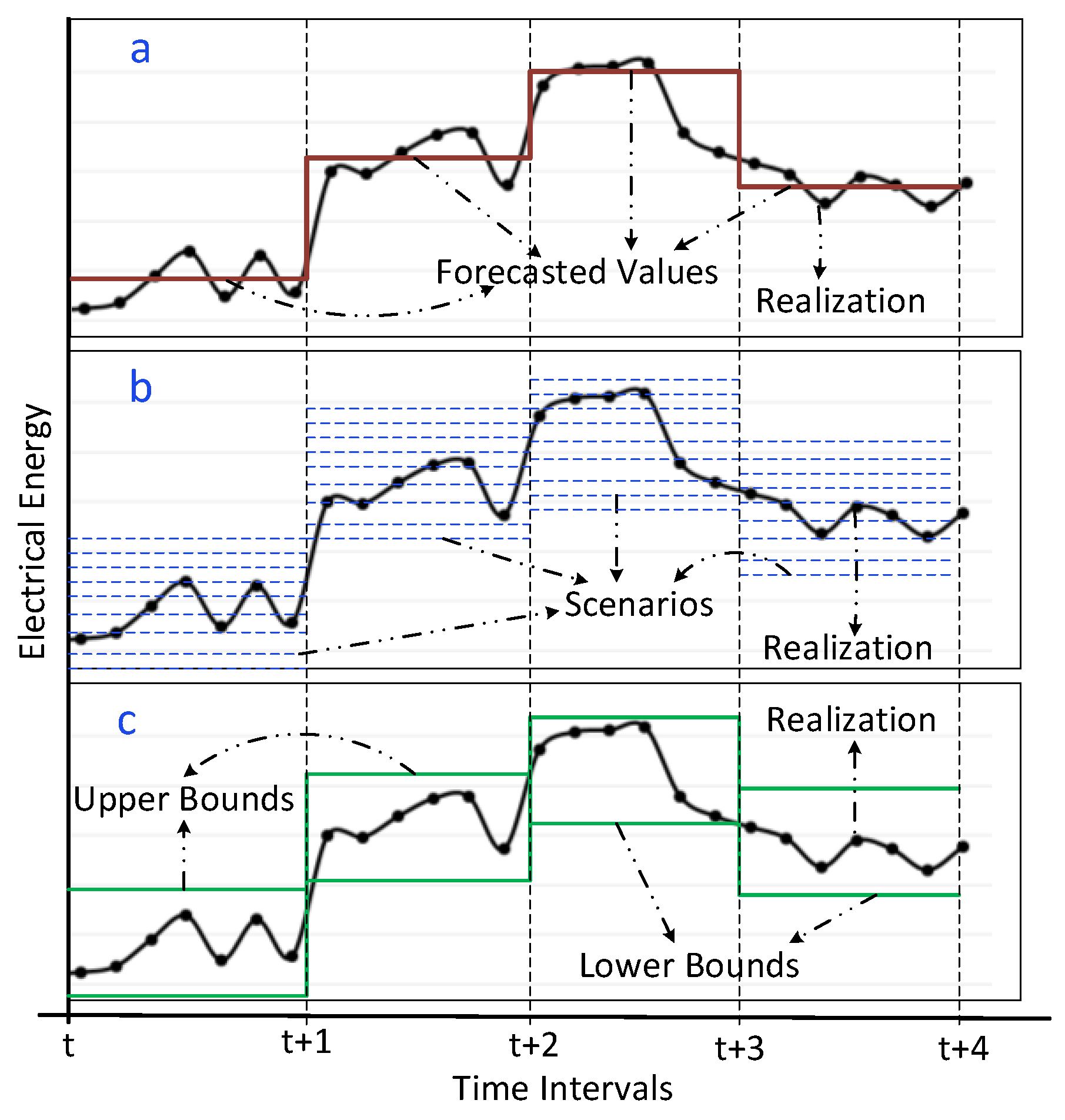
• In case of stochastic optimization, accurate information of uncertainties is required to construct accurate PDFs, while RO describes uncertainties by sets, i.e., upper and lower bounds and need not assume probability distributions [18].
• The accuracy of solution is sensitive to the technique used for scenario generation in stochastic optimization but RO only needs information about the upper and lower bounds [18].

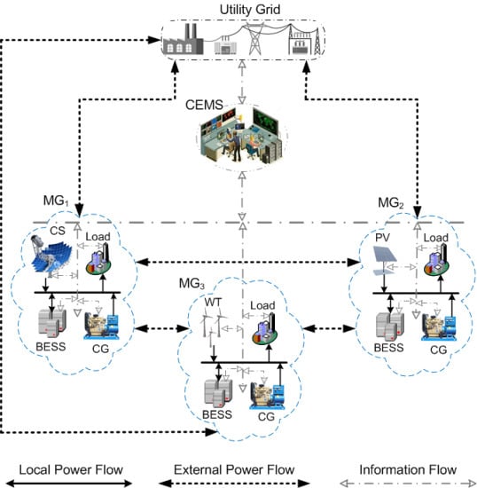
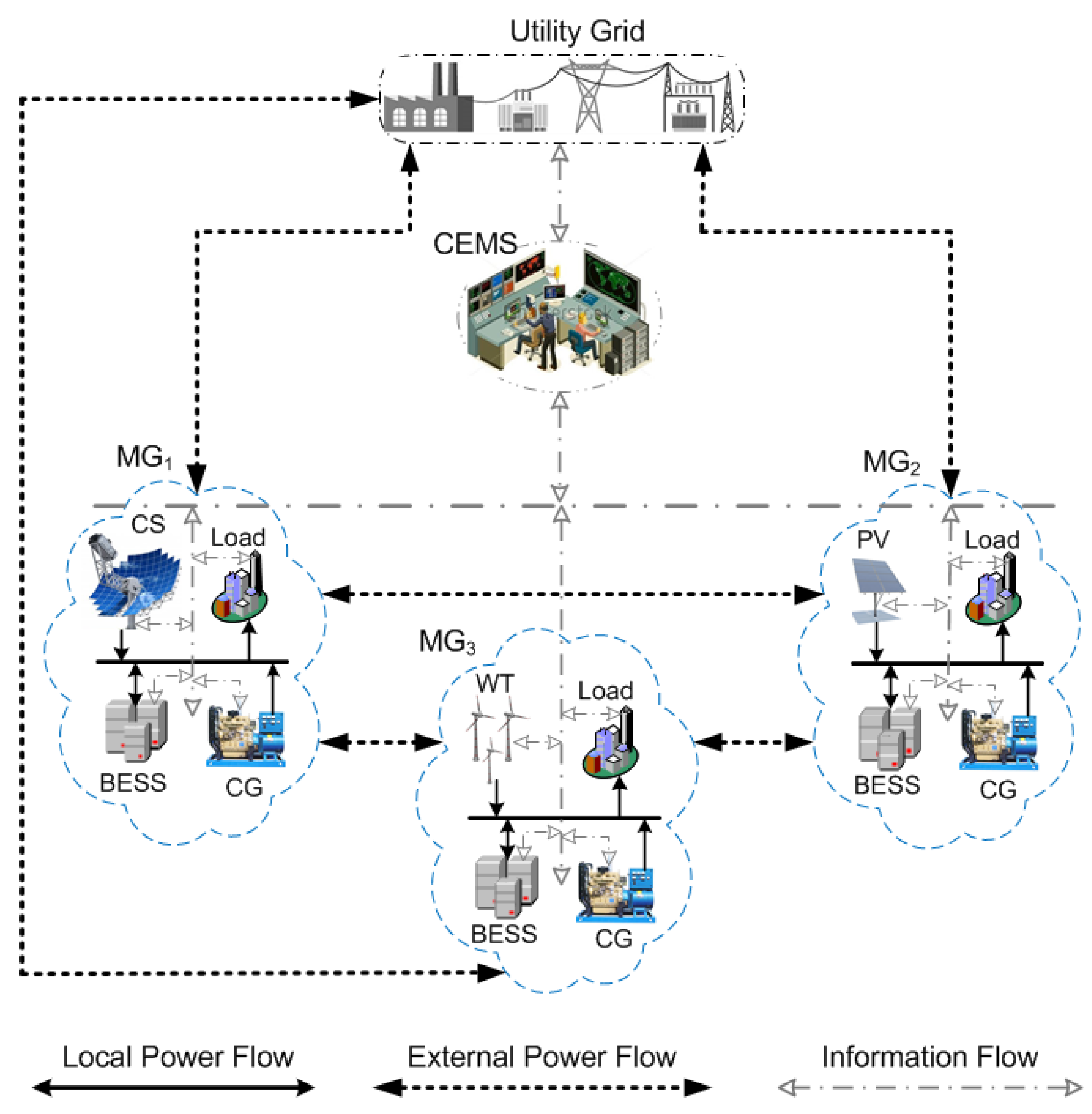
In 1970, Soyster adopted linear robust optimization for the first time. Due to conservativeness under worst-case constraints, this technique has not gained much popularity [18]. These conservative property problems have been resolved by [33], by proposing the concept of adjustable robust optimization. However, the complexity of robust counterpart was still an issue. The complexity issue has been resolved by introducing an adjustable parameter by [34,35]. That parameter has been named as budget of uncertainty and is decided by the decision makers. This parameter can ensure a trade-off between the objective of robustness and economy. This method has been used for optimization of multi-microgrids in this paper.

The breakdown of major steps in a robust optimization-based processing of uncertain data is shown in Figure 2. Estimation of upper and lower uncertainty bounds can be done using historic data [36] or confidence intervals [37]. A review on neural network-based prediction intervals has been carried out by [38] for determining confidence intervals. After determining the upper and lower bounds, a deterministic model is formulated.

The deterministic model is then transformed into the worst-case model. The worst-case model contains a sub-problem; linear duality theory is applied to the sub-problem. By applying Karush-Kuhn-Tucker (KKT) optimality conditions and decided value of budget of uncertainty by decision makers, a traceable robust counterpart can be formulated. The budget of uncertainty is used to formulate a trade-off between the conservatism and the probability of unfeasible solutions within the given uncertainty bounds. The relationship between the error probability of unfeasible solution and budget of uncertainty for independent and symmetrically distributed random variables in $\left[-1,1\right]$ has been formulated by [35].

3. System Model

A cooperative network of three heterogeneous microgrids (MG₁, MG₂, and MG₃) has been considered in this study. The basic components of each microgrid are renewable energy sources (photovoltaic (PV) array, wind turbine (WT), and concentrated solar (CS) power unit), controllable distributed generator (CG), battery energy storage system (BESS), and electric load. Each MG contains at-least one of the three renewable energy sources. CGs in all microgrids are assumed to of same type with different generation capacities. BESS capacity has also been assumed to be different for each MG. All the MGs are inter-connected and connected to the utility grid, such that they can trade energy with the utility grid and with other MGs of the network. Proposed MMG system can also operate in islanded mode. An illustration of the MMG system is shown in Figure 3.

Each MG sends its information to the community EMS (CEMS). This information includes capacity and state of charge (SOC) of BESS, forecasted values of renewable generators with uncertainty bounds, forecasted values of load with uncertainty bounds, and capacity and per-unit generation cost of each CG units. CEMS receives the market price signals (buying and selling prices) from the utility grid. After receiving all the component-related information from each MG and market price signals from the utility grid, CEMS performs optimization of the MMG system with an objective to minimize the operation cost of the MMG system under worst-case realization. CEMS is responsible for scheduling the resources of each MG. Each MG has to follow the scheduling commands received from the CEMS.

4. Problem Formulation

Optimal operation of MGs is considered as the uppermost level of microgrid control. The control levels in MGs are due to difference in significance and time scale for each control level [39]. Each lower level of control is a prerequisite for the upper level control. Therefore, constraints related to the lower levels’ control are assumed to be satisfied in each of the upper level control. The proposed approach is meant for economic scheduling of MMGs, therefore, lower level controls like internal voltage and current control of DRs, voltage and frequency deviations compensation, and load flow analysis, have not been included (assumed to be fulfilled). A robust optimization formulation is developed to deal with the uncertainties of renewable power sources and forecasted load demands. The developed robust model is based on mixed integer linear programming (MILP) and the robustness of the model can be adjusted against the level of conservatism of the solution. The proposed model is formulated for a 24-h scheduling horizon with a time interval of $t$, which could be any uniform interval of time. However, in the proposed scheduling t has been assumed to be one hour.

4.1. Deterministic Model

4.1.1. Objective Function

The objective of the deterministic model is to minimize the following objective function. The objective function comprises the operating costs, start-up and shut-down costs of CGs, total cost of buying electricity from the utility grid, total profit gained by selling electricity to the utility grid in grid-connected mode, and penalty cost for shedding load in islanded mode respectively.$u_m\left(t\right)∊\left\{0,1\right\}$ is operation mode indicator of MMG system.$u_m\left(t\right)$= 1 implies that the m^th MG is connected to the main grid and 0 indicates the islanded mode.

$$\begin{array}{l}\min {\displaystyle \sum _{t=1}^T{\displaystyle \sum _{m=1}^M{\displaystyle \sum _{g=1}^G\left(PU{C}_{m,g}^{CG}\left(p_{m,g}^{CG}\left(t\right)\right)+SU{C}_{m,g}^{CG}\left(t\right)+SD{C}_{m,g}^{CG}\left(t\right)\right)}}}\hfill \\ +{\displaystyle \sum _{t=1}^T{\displaystyle \sum _{m=1}^M\left(C^{BUY}\left(t\right).p_m^{BUY}\left(t\right)-C^{SELL}\left(t\right).p_m^{SELL}\left(t\right)\right)}}.u_m\left(t\right)\hfill \\ +{\displaystyle \sum _{t=1}^T{\displaystyle \sum _{m=1}^M{C}_m^{SHED}}}.p_m^{SHED}\left(t\right).\left(1-u_m\left(t\right)\right)\hfill \end{array}$$

(1)

4.1.2. Load Balancing Constraints

For each MG, the total amount of power generated from the local sources and BESS charging/discharging power must be kept equal to the local load demand and power exchanged with the utility grid and other MGs of the network in grid-connected mode. However, in islanded mode, load shedding might be used for balancing the load as represented by Equation (2a).

$$p_m^{LOAD}\left(t\right)-p_m^{SHED}\left(t\right).\left(1-u_m\left(\mathrm{t}\right)\right)+p_m^{CHR}\left(t\right)+s{t}_m\left(t\right).p_m^{SE}\left(t\right)=p_m^{GEN}\left(t\right)+p_m^{GRID}\left(t\right)+p_m^{DCR}\left(t\right)+r{f}_m\left(t\right).p_m^{RE}\left(t\right);\forall m,t$$

(2a)

$$p_m^{GRID}\left(t\right)=\left(f{g}_m\left(t\right).p_m^{BUY}\left(t\right)-t{g}_m\left(t\right).p_m^{SELL}\left(t\right)\right).u_m\left(\mathrm{t}\right);\forall m,g,t$$

(2b)

$$p_m^{GEN}\left(t\right)={\sum }_{g=1}^G{p}_{m,g}^{CG}\left(t\right)+w{t}_m.p_m^{WT}\left(t\right)+p{v}_m.p_m^{PV}\left(t\right)+c{s}_m.p_m^{CS}\left(t\right);\forall m,t$$

(2c)

$$p{v}_m\left(t\right),w{t}_m\left(t\right),c{s}_m\left(t\right),f{g}_m\left(t\right),t{g}_m\left(t\right),r{f}_m\left(t\right),s{t}_m\left(t\right),u_m\left(\mathrm{t}\right)∊\left\{0,1\right\};\forall m,t$$

(2d)

$$r{f}_m\left(t\right)+s{t}_m\left(t\right)=1;f{g}_m\left(t\right)+t{g}_m\left(t\right)=1;p_m^{SHED}\left(t\right)\le p_m^{LOAD}\left(t\right);\forall m,t$$

(2e)

Equation (2a) is the power balancing equation. While, Equation (2b) shows the trading power with the utility grid and Equation (2c) gives the total local generations (controllable and renewable). Equation (2d) shows the binary variables associated with the renewable generations ($p{v}_m,w{t}_m$,$c{s}_m$), power trading with the utility grid ($f{g}_m,t{g}_m$), and power trading among microgrids ($r{f}_m,s{t}_m$), respectively. Equation (2e) depicts the fact that simultaneous buying/selling from/to the utility grid, and simultaneous sending/receiving to/from other MGs is not possible for a given MG at time$t$.

4.1.3. Constraints for Controllable Generators

Equation (3a)–(3e) show the imposed constraints for distributed controllable generators. In Equation (3a), $s_{m,g}\left(t\right)$ is a binary variable and it shows the commitment status of $CGg$ in $MGm$ at time interval $t.$ If CG is committed to operate in time$t$, this binary variable takes the value of $1$and $0$otherwise. Power generation limits of g^th CG in m^th MG are given by Equation (3a). Equation (3b) shows the relationship between the start-up indicator ($s{u}_{m,g}\left(t\right)$) and shut-down indicator ($s{d}_{m,g}\left(t\right)$). If the g^th CG is started up at time$t$, start-up indicator will take the value of 1 and zero otherwise. Similarly, the shutdown indicator will take a value of 1, if the g^th CG is shut-down at time t and zero otherwise [30]. Equation (3c) and (3d) show the constraints related to start-up and shut-down costs, respectively. Equation (3e) portrays the fact that at any given time $t$, any CG cannot be started up and shut down simultaneously.

$$min\left[P_{m,g}^{CG}\right].s_{m,g}\left(t\right)\le p_{m,g}^{CG}\left(t\right)\le max\left[P_{m,g}^{CG}\right].s_{m,g}\left(t\right);s_{m,g}\left(t\right)∊\left\{0,1\right\};\forall m,g,t$$

(3a)

$$s{u}_{m,g}\left(t\right)-s{d}_{m,g}\left(t\right)=s_{m,g}\left(t\right)-s_{m,g}\left(t-1\right);\forall m,g,t$$

(3b)

$$SU{C}_{m,g}^{CG}\left(t\right)\ge U{C}_{m,g}^{CG}\left(t\right).\left(s_{m,g}\left(t\right)-s_{m,g}\left(t-1\right)\right);SU{C}_{m,g}^{CG}\left(t\right)\ge 0;\forall m,g,t$$

(3c)

$$SD{C}_{m,g}^{CG}\left(t\right)\ge D{C}_{m,g}^{CG}\left(t\right).\left(s_{m,g}\left(t-1\right)-s_{m,g}\left(t\right)\right);SD{C}_{m,g}^{CG}\left(t\right)\ge 0;\forall m,g,t$$

(3d)

$$s{u}_{m,g}\left(t\right)+s{d}_{m,g}\left(t\right)\le 1;s{u}_{m,g}\left(t\right),s{d}_{m,g}\left(t\right)∊\left\{0,1\right\};\forall m,g,t$$

(3e)

4.1.4. Energy Trading Constraints

The power exchange between the m^th MG and utility grid is limited by the capacity of the corresponding line connecting them. Equation (4a) shows this limitation for trading power with the utility grid. The binary variables as defined in Equation (2e) allow the m^th MG to either buy or sell power from/to the utility grid at a given time interval $t$. The value of $p_m^{GRID}\left(t\right)$ will be positive if the MG buys powers from the utility grid and will be negative if the MG sells power to the utility grid at any time interval $t$ [30].

$$-P_m^{CAP}\le p_m^{GRID}\left(t\right)\le P_m^{CAP};\forall m,t$$

(4a)

$$0\le p_{\left(m,n\right)}^{SE}\left(t\right)\le s{t}_m\left(t\right).P_{\left(m,n\right)}^{CAP};\forall m,n,t;\forall m\ne n$$

(4b)

$$0\le p_{\left(m,n\right)}^{RE}\left(t\right)\le r{f}_m\left(t\right).P_{\left(m,n\right)}^{CAP};\forall m,n,t;\forall m\ne n$$

(4c)

$$0\le p_{\left(m,n\right)}^{RE}\left(t\right)\le p_m^{DEF}\left(t\right);\forall m,n,t;\forall m\ne n$$

(4d)

$$0\le p_{\left(m,n\right)}^{SE}\left(t\right)\le p_m^{SUR}\left(t\right);\forall m,n,t;\forall m\ne n$$

(4e)

$${\sum }_{m=1}^M{\sum }_{n=1}^N{p}_{\left(m,n\right)}^{RE}\left(t\right)={\sum }_{n=1}^N{\sum }_{m=1}^M{p}_{\left(n,m\right)}^{RE}\left(t\right);\forall m,n,t;\forall m\ne n$$

(4f)

The power exchange between any two connected MGs (m and n) is limited by the capacity of the corresponding line connecting them. Equation (4b) and (4c) show these limitations for sending power from m^th MG to n^th MG and receiving power by m^th MG from n^th MG, respectively. The value of $p_{\left(m,n\right)}^{SE}\left(t\right)$ will be positive, if MG m sends power to MG n and it will be zero otherwise. Similarly, the value of $p_{\left(m,n\right)}^{RE}\left(t\right)$ will be positive if MG m receives power from MG n and vice versa. Equation (2e) allows each MG to either send or receive power at time interval$t$. Equation (4d) constraints each MG for receiving only deficit amount of power from other microgrids, i.e., prohibits selling of received power and (4e) restricts each MG for sending only surplus power to other MGs of the network, i.e., prohibits from buying while sending power. Finally, Equation (4f) shows that amount of power sent and received to/from MGs of network should be balanced at each time interval$t$.

4.1.5. Battery Constraints

The limits and dynamics of electrical energy stored in the BESS of m^th MG are given by Equation (5a) and (5b). Equation (5c) and (5d) show the charging and discharging limits of BESS, respectively. Equation (5e) shows the constraints related to initial step of the simulation time frame with $P_m^{INIT}$ as the initial SOC of the BESS. Equation (5f) depicts that BESS cannot be charged and discharged simultaneously. The time interval (time step) for BESS modeling will be in accordance to defined time step in problem formulation, i.e., one hour in this study.

$$\text{min}\left[P_m^{BESS}\right]\le p_m^{SOC}\left(t\right)\le \text{max}\left[P_m^{BESS}\right];\forall m,t$$

(5a)

$$p_m^{SOC}\left(t\right)=p_m^{SOC}\left(t-1\right)+p_m^{CHR}\left(t\right).{\eta }_m^{CHR}-\frac{p_m^{DCR}\left(t\right)}{{\eta }_m^{DCR}};\forall m,t$$

(5b)

$$0\le p_m^{CHR}\left(t\right)\le \left(\frac{\text{max}\left[P_m^{BESS}\right]-p_m^{SOC}\left(t-1\right)}{{\eta }_m^{CHR}}\right).c_m\left(t\right);\forall m,t$$

(5c)

$$0\le p_m^{DCR}\left(t\right)\le \left(\left(p_m^{SOC}\left(t-1\right)-\text{ min}\left[P_m^{BESS}\right]\right)\right).{\eta }_m^{DCR}.d_m\left(t\right);\forall m,t$$

(5d)

$$p_m^{SOC}\left(t-1\right)=P_m^{INIT}ift=1;\forall m,t$$

(5e)

$$c_m\left(t\right)+d_m\left(t\right)=1;c_m\left(t\right),d_m\left(t\right)∊\left\{0,1\right\};0\le {\eta }_m^{CHR},{\eta }_m^{DCR}\le 1;\forall m,t$$

(5f)

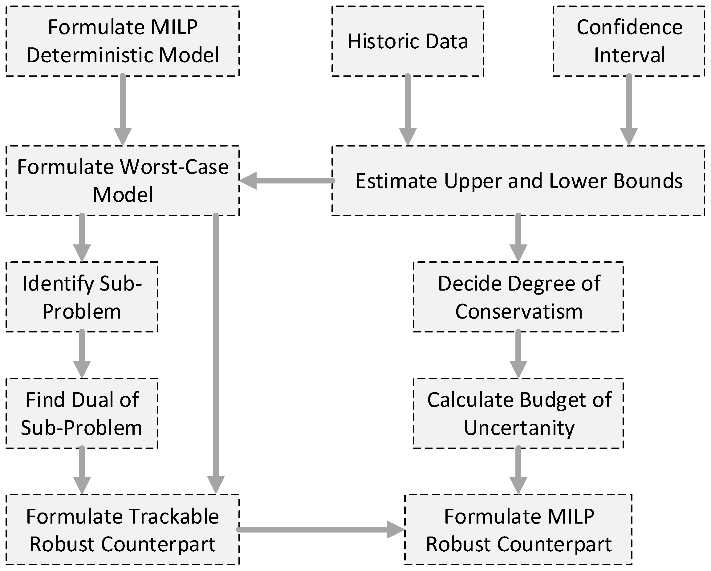
4.2. Robust Counterpart

The next step in robust optimization-based problem solving is to formulate a robust counterpart of the deterministic model as depicted by Figure 2. The purpose of the robust counterpart is to overcome the drawbacks introduced by uncertainties [40]. The uncertainty bounds are formulated prior to worst-case model realization, in order to cater the influence of intermittent renewable power generation and variable customer loads.

4.2.1. Uncertainty Bounds

It is assumed that all the decision variables should be made before the revealing of the uncertainty from the renewable energy sources and electric loads. The bounded variables for electric load (${\widehat{p}}_m^{LOAD}\left(t\right)$) and renewables power generations (${\widehat{p}}_m^{PV}\left(t\right)$, ${\widehat{p}}_m^{WT}\left(t\right)$, ${\widehat{p}}_m^{CS}\left(t\right)$) are given by Equation (6a)–(6d). The symmetrical uncertainties associated with load ($∆p_m^{LOAD}\left(t\right)$) and renewable power generations ($∆p_m^{PV}\left(t\right),∆p_m^{WT}\left(t\right),∆p_m^{CS}\left(t\right)$) lie within the upper and lower bounds given by Equation (6a)–(6d). The upper bounds (${\overline{p}}_m^{LOAD}\left(t\right),{\overline{p}}_m^{PV}\left(t\right),{\overline{p}}_m^{WT}\left(t\right),{\overline{p}}_m^{CS}\left(t\right)$) and lower bounds (${\underset{\_}{p}}_m^{LOAD}\left(t\right),{\underset{\_}{p}}_m^{PV}\left(t\right),{\underset{\_}{p}}_m^{WT}\left(t\right),{\underset{\_}{p}}_m^{CS}\left(t\right)$) for the uncertain quantities (load and renewable generators) can be calculated using the methods suggested by [36,37,38].

$${\widehat{p}}_m^{LOAD}\left(t\right)=p_m^{LOAD}+∆p_m^{LOAD}\left(t\right);{\underset{\_}{p}}_m^{LOAD}\left(t\right)\le ∆p_m^{LOAD}\left(t\right)\le {\overline{p}}_m^{LOAD}\left(t\right);\forall m,t$$

(6a)

$${\widehat{p}}_m^{PV}\left(t\right)=p_m^{PV}+∆p_m^{PV}\left(t\right);{\underset{\_}{p}}_m^{PV}\left(t\right)\le ∆p_m^{PV}\left(t\right)\le {\overline{p}}_m^{PV}\left(t\right);\forall m,t$$

(6b)

$${\widehat{p}}_m^{WT}\left(t\right)=p_m^{WT}+∆p_m^{WT}\left(t\right);{\underset{\_}{p}}_m^{WT}\left(t\right)\le ∆p_m^{WT}\left(t\right)\le {\overline{p}}_m^{WT}\left(t\right);\forall m,t$$

(6c)

$${\widehat{p}}_m^{CS}\left(t\right)=p_m^{CS}+∆p_m^{CS}\left(t\right);{\underset{\_}{p}}_m^{CS}\left(t\right)\le ∆p_m^{CS}\left(t\right)\le {\overline{p}}_m^{CS}\left(t\right);\forall m,t$$

(6d)

4.2.2. Load Balancing

The objective function of robust model is identical to that of deterministic model (1). The electric power balance in each microgrid should be met when the worst-case of uncertainties occur. The worst-case for the load balancing in deterministic model (2a) for m^th MG would occur at the maximum increase in the electric load and maximum decrease in the renewable power generation. The worst-case load balancing is depicted by Equation (7a) with $p_m^{WC}\left(t\right)$ as the total uncertainty factor. The total uncertainty factor can be calculated using Equation (7b).

$$p_m^{LOAD}\left(t\right)-p_m^{SHED}\left(t\right).\left(1-u_m\left(\mathrm{t}\right)\right)+p_m^{CHR}\left(t\right)+s{t}_m\left(t\right).p_m^{SE}\left(t\right)+p_m^{WC}\left(t\right)=p_m^{GEN}\left(t\right)+p_m^{GRID}\left(t\right)+p_m^{DCR}\left(t\right)+r{f}_m\left(t\right).p_m^{RE}\left(t\right);\forall m,t$$

(7a)

$$p_m^{WC}\left(t\right)=max\left\{\begin{array}{c}\left({\underset{\_}{p}}_m^{LOAD}\left(t\right).{\underset{\_}{z}}_m^{LOAD}\left(t\right)+{\overline{p}}_m^{LOAD}\left(t\right).{\overline{z}}_m^{LOAD}\left(t\right)\right)-\\ p{v}_m.\left({\underset{\_}{p}}_m^{PV}\left(t\right).{\underset{\_}{z}}_m^{PV}\left(t\right)+{\overline{p}}_m^{PV}\left(t\right).{\overline{z}}_m^{PV}\left(t\right)\right)-\\ w{t}_m.\left({\underset{\_}{p}}_m^{WT}\left(t\right).{\underset{\_}{z}}_m^{WT}\left(t\right)+{\overline{p}}_m^{WT}\left(t\right).{\overline{z}}_m^{WT}\left(t\right)\right)-\\ c{s}_m.\left({\underset{\_}{p}}_m^{CS}\left(t\right).{\underset{\_}{z}}_m^{CS}\left(t\right)+{\overline{p}}_m^{CS}\left(t\right).{\overline{z}}_m^{CS}\left(t\right)\right)\end{array}\right\};\forall m,t$$

(7b)

4.3. Sub-Problen and Dual

The next step in robust optimization-based problem solving is to identify the sub-problem and find dual of the sub-problem. It can be observed from the worst-case load balancing Equation (7a) and (7b) that maximization of uncertainty factor is a new objective inside the load balancing equation. The sub-problem can be formulated by taking Equation (7b) as the objective function and Equation (8a) and (8b) as the constraints.

$$\begin{array}{l}\left\{\begin{array}{c}\left({\underset{\_}{z}}_m^{LOAD}\left(t\right)+{\overline{z}}_m^{LOAD}\left(t\right)\right)+w{t}_m.\left({\underset{\_}{z}}_m^{WT}\left(t\right)+{\overline{z}}_m^{WT}\left(t\right)\right)+\\ p{v}_m.\left({\underset{\_}{z}}_m^{PV}\left(t\right)+{\overline{z}}_m^{PV}\left(t\right)\right)+c{s}_m.\left({\underset{\_}{z}}_m^{CS}\left(t\right)+{\overline{z}}_m^{CS}\left(t\right)\right)\end{array}\right\}\le {\Gamma }_m\left(t\right)\in \left[0,k\right];\forall m,t\end{array}$$

(8a)

$$\begin{array}{c}0\le {\underset{\_}{z}}_m^{WT}\left(t\right),{\overline{z}}_m^{WT}\left(t\right),{\underset{\_}{z}}_m^{PV}\left(t\right),{\overline{z}}_m^{PV}\left(t\right),\\ {\underset{\_}{z}}_m^{CS}\left(t\right),{\overline{z}}_m^{CS}\left(t\right),{\underset{\_}{z}}_m^{LOAD}\left(t\right),{\overline{z}}_m^{LOAD}\left(t\right)\le 1;\forall m,t\end{array}$$

(8b)

The variables (${\underset{\_}{z}}_m^{LOAD}\left(t\right),{\overline{z}}_m^{LOAD}\left(t\right)$), (${\underset{\_}{z}}_m^{WT}\left(t\right),{\overline{z}}_m^{WT}\left(t\right)$), (${\underset{\_}{z}}_m^{PV}\left(t\right),{\overline{z}}_m^{PV}\left(t\right)$. ), and (${\underset{\_}{z}}_m^{CS}\left(t\right),{\overline{z}}_m^{CS}\left(t\right)$) are the scaled deviations for random electric loads, random wind power generation, random solar power generation, and random concentrated solar power generations, respectively. ${Г}_m\left(t\right)$ is the budget of uncertainty of m^th MG and is used to adjust the range of uncertainty set for electric loads and renewable power generation at time t [40].

In order to make the robust counterpart tractable, the sub-problem, which is composed of Equations (7b), (8a) and (8b), needs to be converted into the dual problem. By applying the linear duality theory and KKT optimality conditions on the sub-problem, following equations can be formulated.

$$min\left\{\begin{array}{c}{\zeta }_m\left(t\right).{\Gamma }_m\left(t\right)+\left({\lambda }_m^{l+}\left(t\right)+{\lambda }_m^{l-}\left(t\right)\right)+p{v}_m.\left({\lambda }_m^{p+}\left(t\right)+{\lambda }_m^{p-}\left(t\right)\right)+\\ w{t}_m.\left({\lambda }_m^{w+}\left(t\right)+{\lambda }_m^{w-}\left(t\right)\right)+c{s}_m.\left({\lambda }_m^{c+}\left(t\right)+{\lambda }_m^{c-}\left(t\right)\right)\end{array}\right\};\forall m,t$$

(9a)

$${\mathsf{\zeta }}_m\left(t\right)+{\lambda }_m^{l-}\left(t\right)\ge {\underset{\_}{p}}_m^{LOAD}\left(t\right);{\mathsf{\zeta }}_m\left(t\right)+{\lambda }_m^{l+}\left(t\right)\ge {\overline{p}}_m^{LOAD}\left(t\right);\forall m,t$$

(9b)

$${\mathsf{\zeta }}_m\left(t\right)+{\lambda }_m^{w-}\left(t\right)\ge -w{t}_m.{\underset{\_}{p}}_m^{WT}\left(t\right);{\mathsf{\zeta }}_m\left(t\right)+{\lambda }_m^{w+}\left(t\right)\ge -w{t}_m.{\overline{p}}_m^{WT}\left(t\right);\forall m,t$$

(9c)

$${\mathsf{\zeta }}_m\left(t\right)+{\lambda }_m^{p-}\left(t\right)\ge -p{v}_m.{\underset{\_}{p}}_m^{PV}\left(t\right);{\mathsf{\zeta }}_m\left(t\right)+{\lambda }_m^{p+}\left(t\right)\ge -p{v}_m.{\overline{p}}_m^{PV}\left(t\right);\forall m,t$$

(9d)

$${\mathsf{\zeta }}_m\left(t\right)+{\lambda }_m^{c-}\left(t\right)\ge -c{s}_m.{\underset{\_}{p}}_m^{CS}\left(t\right);{\mathsf{\zeta }}_m\left(t\right)+{\lambda }_m^{c+}\left(t\right)\ge -c{s}_m.{\overline{p}}_m^{CS}\left(t\right);\forall m,t$$

(9e)

$${\mathsf{\zeta }}_m\left(t\right),{\lambda }_m^{l+}\left(t\right),{\lambda }_m^{l-}\left(t\right),{\lambda }_m^{p+}\left(t\right),{\lambda }_m^{p-}\left(t\right),{\lambda }_m^{w+}\left(t\right),{\lambda }_m^{w-}\left(t\right),{\lambda }_m^{c+}\left(t\right),{\lambda }_m^{c-}\left(t\right)\ge 0;\forall m,t$$

(9f)

In order to convert the sub-problem into dual problem, dual variables are required. Dual variables for load (${\lambda }_m^{l+}\left(t\right),{\lambda }_m^{l-}\left(t\right)$), wind power generators (${\lambda }_m^{w+}\left(t\right),{\lambda }_m^{w-}\left(t\right)$), solar power generators (${\lambda }_m^{p+}\left(t\right),{\lambda }_m^{p-}\left(t\right)$), concentrated solar power generators (${\lambda }_m^{c+}\left(t\right)+{\lambda }_m^{c-}\left(t\right)$), and uncertainty adjustment factor (${\mathsf{\zeta }}_m\left(t\right)$) have been introduced in Equation (9a)–(9f). It can be observed from above equation set that Equation (9a) is the dual objective function of the sub-problem. While Equation (9b)–(9f) are the dual constraints subjected to the dual objective function. Equation (9f) depicts the fact that all the dual variables are non-negative.

4.4. Tractable Robust Counterpart

The final step in robust optimization-based problem solving is to formulate a tractable robust counterpart of the non-linear robust model as depicted by Figure 2. By using the dual problem developed in previous section and the worst-case load balancing Equation (7a), final tractable robust counterpart can be formulated as following:

$$\begin{array}{l}\min {\displaystyle \sum _{t=1}^T{\displaystyle \sum _{m=1}^M{\displaystyle \sum _{g=1}^G\left(PU{C}_{m,g}^{CG}\left(p_{m,g}^{CG}\left(t\right)\right)+SU{C}_{m,g}^{CG}\left(t\right)+SD{C}_{m,g}^{CG}\left(t\right)\right)}}}\hfill \\ +{\displaystyle \sum _{t=1}^T}{\displaystyle \sum _{m=1}^M}(C^{BUY}\left(t\right).p_m^{BUY}\left(t\right)-C^{SELL}\left(t\right).p_m^{SELL}\left(t\right)).u_m\left(t\right)\hfill \\ +{\displaystyle \sum _{t=1}^T{\displaystyle \sum _{m=1}^M{C}_m^{SHED}}}.p_m^{SHED}\left(t\right).\left(1-u_m\left(t\right)\right)\hfill \end{array}$$

(10)

Subject to:

$$p_m^{LOAD}\left(t\right)–p_m^{SHED}\left(t\right).\left(1-u_m\left(\mathrm{t}\right)\right)+p_m^{CHR}\left(t\right)+s{t}_m\left(t\right).p_m^{SE}\left(t\right)+p_m^{DU}\left(t\right)=p_m^{GRID}\left(t\right)+p_m^{DCR}\left(t\right)+r{f}_m\left(t\right).p_m^{RE}\left(t\right);\forall m,t$$

(11a)

$$p_m^{DU}\left(t\right)=\left\{\begin{array}{c}{\zeta }_m\left(t\right).{\Gamma }_m\left(t\right)+\left({\lambda }_m^{l-}\left(t\right)+{\lambda }_m^{l+}\left(t\right)\right)+p{v}_m.\left({\lambda }_m^{p-}\left(t\right)+{\lambda }_m^{p+}\left(t\right)\right)+\\ w{t}_m.\left({\lambda }_m^{w-}\left(t\right)+{\lambda }_m^{w+}\left(t\right)\right)+c{s}_m.\left({\lambda }_m^{c-}\left(t\right)+{\lambda }_m^{c+}\left(t\right)\right)\end{array}\right\};\forall m,t$$

(11b)

and Equations (2a)–(2e), (3a)–(3e), (4a)–(4f), (5a)–(5e), and (9b)–(9f).

It can be observed from Equation (10) that the objective function is identical to that of the deterministic model (Equation (1)). The value of budget of uncertainty is decided by the decision makers. Once the value of ${Г}_m\left(t\right)$is known, the tractable robust counter-part can be implemented using commercial software like CPLEX, which guarantee global optimality for MILP problems. A formulation has been derived by [35] for determining ${Г}_m\left(t\right)$ with a given error probability.

5. Numerical Simulations

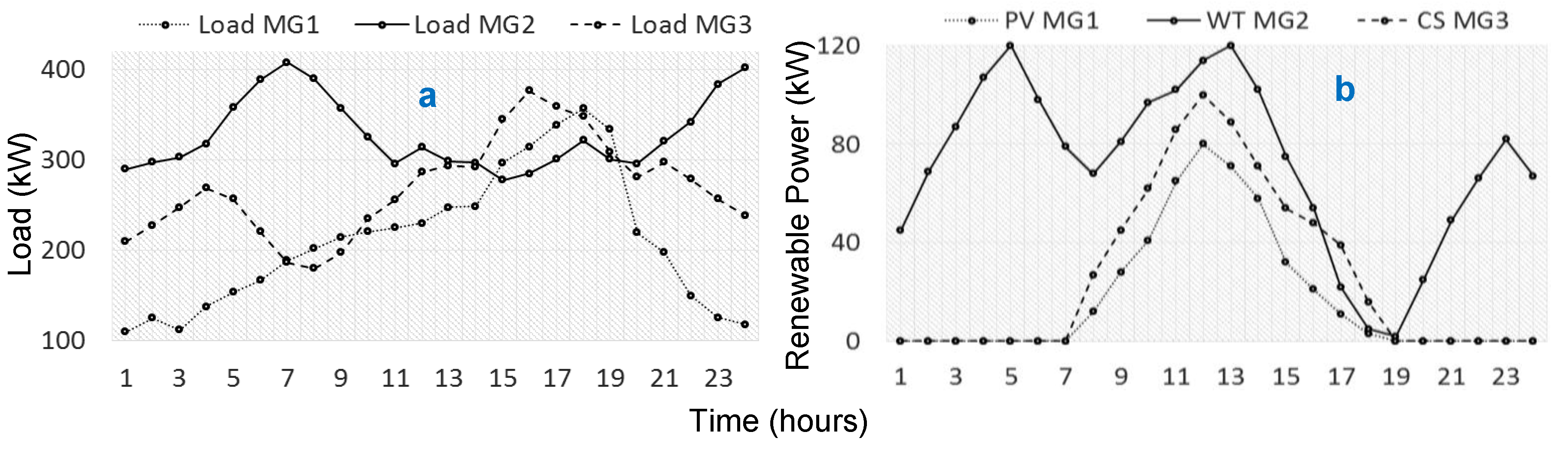
The developed RO-based scheduling algorithm has been applied to a multi-microgrid system composed of three microgrids as shown in Figure 3. The analysis has been conducted for a 24 h scheduling horizon with a time interval of 1 h. All the numerical simulations have been coded in C++ in Microsoft visual studio environment using CPLEX 12.3.

In order to visualize the uncertainty impact of both renewable energy sources and load, three cases have been simulated in this study. In the first case, nominal values of load have been considered with uncertain renewable power outputs. The second case elaborates the effects of uncertainty in load only, while the third case considers uncertainty in both renewable power output and load in both of the operation modes of MGs. Finally, operation costs have been compared against different values of ${Г}_m\left(t\right)$ for each case. The maximum value of ${Г}_m\left(t\right)$ depends on the number of uncertain random variables in that interval of time. Therefore, ${Г}_m\left(t\right)$ will take a maximum value of 1 for initial two cases, where only one uncertainty source (renewable power generator or electric load) is considered, while the maximum value of ${Г}_m\left(t\right)$ will be 2 for the third case, where both of the uncertainty sources (renewable power generator and electric load) are considered. The realization where ${Г}_m\left(t\right)$ takes its respective maximum value is termed as worst-case realization under those conditions.

5.1. Input Data

The forecasted hourly load profile of each MG is shown is Figure 4a, while Figure 4b shows the hourly output powers of non-dispatchable generators. The parameters related to BESSs, CGs and RGs are listed in

Table 1. Parameters related to energy resources in each MG.

MGs	Capacities and Parameters of BESSs				Generation Limits of CGs		Generation Capacities of RGs
	${\mathit{\eta }}_{\mathit{m}}^{\mathit{C}\mathit{H}\mathit{R}}$	${\mathit{\eta }}_{\mathit{m}}^{\mathit{D}\mathit{C}\mathit{R}}$	$\mathit{m}\mathit{i}\mathit{n}\mathbf{\left[}{\mathit{P}}_{\mathit{m}}^{\mathit{B}\mathit{E}\mathit{S}\mathit{S}}\mathbf{\right]}$	$\mathit{m}\mathit{a}\mathit{x}\mathbf{\left[}{\mathit{P}}_{\mathit{m}}^{\mathit{B}\mathit{E}\mathit{S}\mathit{S}}\mathbf{\right]}$	$\mathit{min}\mathbf{\left[}{\mathit{P}}_{\mathit{m}\mathbf{,}\mathit{g}}^{\mathit{C}\mathit{G}}\mathbf{\right]}$	$\mathit{max}\mathbf{\left[}{\mathit{P}}_{\mathit{m}\mathbf{,}\mathit{g}}^{\mathit{C}\mathit{G}}\mathbf{\right]}$	PV	WT	CS
MG1	2%	2%	0 kWh	80 kWh	0 kWh	230 kWh	80 kWh	-	-
MG2	2%	2%	0 kWh	50 kWh	170 kWh	340 kWh	-	120 kWh	-
MG3	2%	2%	0 kWh	70 kWh	0 kWh	300 kWh	-	-	90 kWh
Total	6%	6%	0 kWh	200 kWh	170 kWh	870 kWh	80 kWh	120 kWh	90 kWh

.

Uncertainty bounds in electric loads have been taken from [41] and renewable generation uncertainty bounds have been considered ±10% wider than [41]. The value of uncertainty gap can be calculated using the value of corresponding ${Г}_m\left(t\right)$ and forecasted values of corresponding uncertain variables. All quantities in Figure 5, Figure 6, Figure 7, Figure 8, Figure 9, Figure 10, Figure 11, Figure 12, Figure 13 and Figure 14 have been calculated by adding the corresponding quantities of individual microgrids, i.e., collective/cumulative values. The collective uncertainty gap while considering uncertainty of renewable power sources only is shown in Figure 5a and load only in Figure 5b. The uncertainty gap shown is Figure 6a has been calculated by considering uncertainties in both renewable power sources and electric loads. Day-ahead market price signals have been taken as inputs and are depicted by Figure 6b.

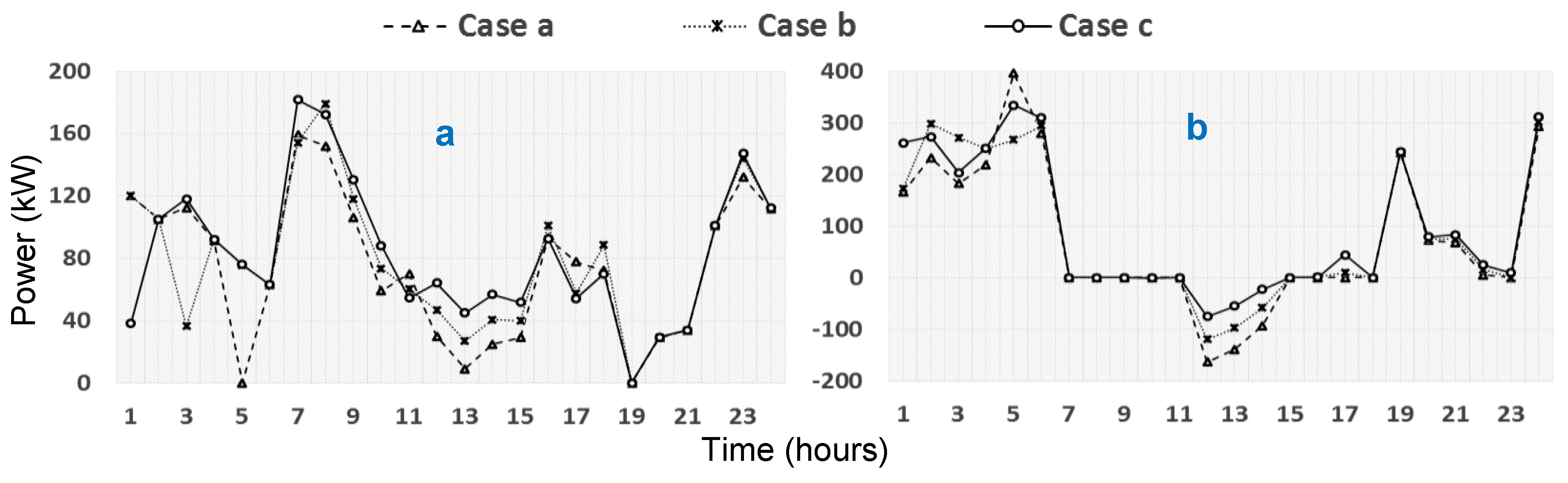
5.2. Uncertainty in Renewable Energy Sources

The multi-microgrid scheduling problem has been solved by considering uncertainty in renewable power sources only in this section. The uncertainty gap for this case is shown in Figure 5a. Three cases have been considered for comparing internal and external trading, generation of CGs, and charging/discharging of BESS elements. Case a is the deterministic case (${Г}_m\left(t\right)=0$), Case c is the worst-case (${Г}_m\left(t\right)=1$), and Case b is an intermediate case (${Г}_m\left(t\right)=0.5$) in this section.

It can be observed from Figure 5a that uncertainty gap for Case a (deterministic case) is zero. However, an uncertainty gap can be observed for Case b and even a wider gap for Case c. This uncertainty gap has to be filled by the CEMS through external trading (trading with utility grid), internal trading (trading among microgrids), increasing the generation of CGs, and/or by utilizing BESSs.

Case b: It can be observed from Figure 7b that in time intervals 1–4, 6, and 24, uncertainty gap has been filled by buying more power from the utility grid. Figure 8a shows that CG generation has been increased in the time intervals 8–11, 15, 16, and 23 to fulfill the gap. Figure 7a shows that amount of selling power has been reduce in time intervals 12–14 to suffice the energy needs of microgrids. Figure 8b shows that BESSs have been charged in the initial off-peak price intervals and discharged in the peak intervals of price. Figure 7a shows that internal trading is increased when CG generation is increased or BESS is discharged. Such type of behavior can be observed in time intervals 8–11, 16, 16, 23 and 15–18, respectively.

Case c: The uncertainty gap of Case c is wider than that of Case b as shown in Figure 5a. Therefore, Case c realization requires more generation or internal/external trading to assure the feasibility of solution even in the worst-case scenario. However, Figure 7 and Figure 8 depict that the general behavior of Case c is similar to that of Case b. The driving force of this behavior is the minimization of the operation cost which can be achieved by buying from utility grid and charging BESSs in off-peak price intervals, increasing generation of CGs in the mid-peak price intervals, and increasing the selling to the utility grid and discharging BESS in the peak price intervals.

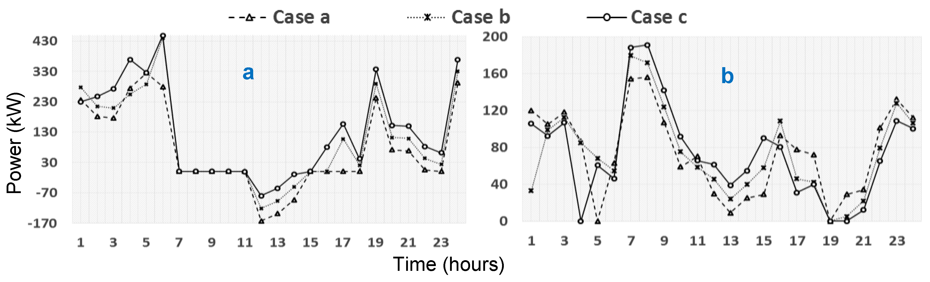
5.3. Uncertainty in Electric Load

In this section, the multi-microgrid scheduling problem has been solved by considering uncertainty in electric loads only. The hour-wise uncertainty gap is shown in Figure 5b. In this section also, three cases have been considered. Case a is the deterministic case (load with nominal values), Case c is the worst-case (load increased by 10%) and Case b is an intermediate case (load increased by 5%). The trend of uncertainty gap is different from that of Section 5.2 where, due to uncertainty in renewable energy sources, maximum uncertainty can be observed at the noon time. However, due to the presence of load in all the time intervals the uncertainty is comparatively uniform and can be observed from Figure 5b.

Case b: It can be observed from Figure 9a that buying from the utility grid has increased in the time intervals 1–6, and 24. In the mid-peak price interval generation cost of MG₁ is lower than the market buying price and that of MG₂ lies between the selling and buying prices, which can be observed from Figure 6b. Therefore, MG₂ increases its generation in time intervals 7–11 as shown in Figure 10a. However, due to higher magnitude of loads in time intervals 19–23, external trading (buying from utility grid) has increased in these time intervals. In deterministic case, MG₁ and MG₂ generate to their fullest in the peak price intervals 12–15 and sell the surplus amount of power to the utility grid. However, cost of CG in MG₃, being sandwiched between the buying and selling prices, only generated required amount (neither buying nor selling). Figure 9a shows that external trading has significantly reduced in the peak price intervals. BESS has been charged and discharged twice in this case as shown in Figure 10b and internal trading has increased in most of the time intervals as shown in Figure 9b.

Case c: It is the worst-case scenario, i.e., loads of all the MGs take their worst values. Figure 5b shows that uncertainty gap is higher in this case as compared to Case b. The general trend is similar to that of Case b, with elevated magnitudes. The general trend of MMG is decided by the market price signals and per-unit generation cost of CGs in each MG. It can be observed from Figure 6b that during off-peak price interval MG₁ has generated maximum power but MG₂ and MG₃ have generated minimum power and bought the deficit amount from the utility grid. In the mid-peak price intervals MG₁ and MG₂ have generated maximum and MG₃ has generated as per requirement. BESSs are charged in off and mid-peak price intervals and are used in mid or on-peak price intervals.

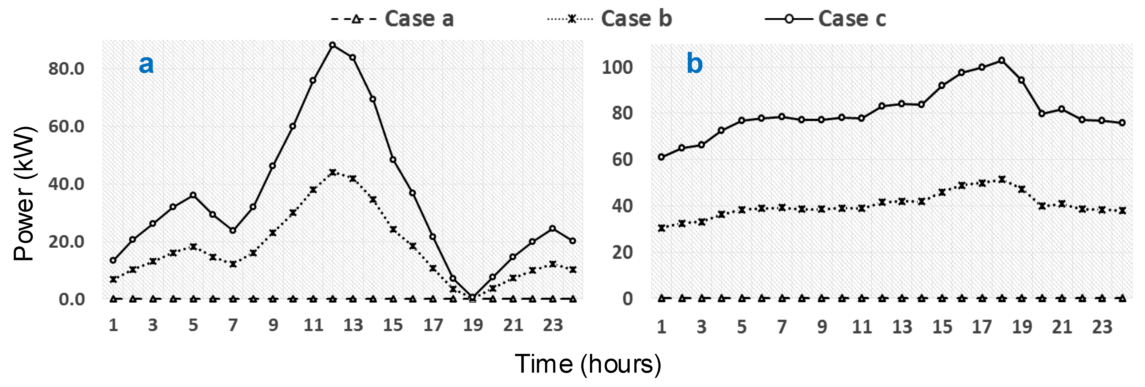
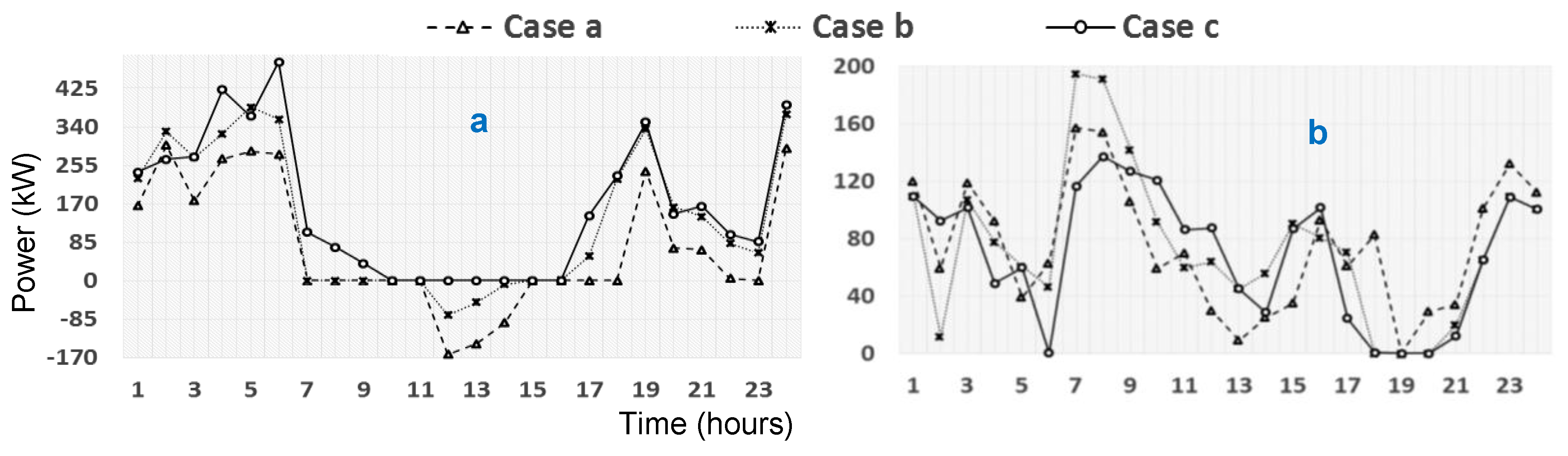
5.4. Uncertainty in both Renewable Energy Sources and Electric Load

In the final case, the multi-microgrid scheduling problem has been solved by considering uncertainties in both renewable power sources and electric loads. The uncertainty gaps for this case are shown in Figure 6a. Similar to previous sections, in this section also, three cases have been considered. Case a is the deterministic case (${Г}_m\left(t\right)=0$), Case c is the worst-case (${Г}_m\left(t\right)=2$), and Case b is an intermediate case (${Г}_m\left(t\right)=1$). There are two sets of random variables in this case. One set is associated with the load and other with the renewable power sources. The general trend of uncertainty gap shown in Figure 6a reflects the behavior of both of the previous cases.

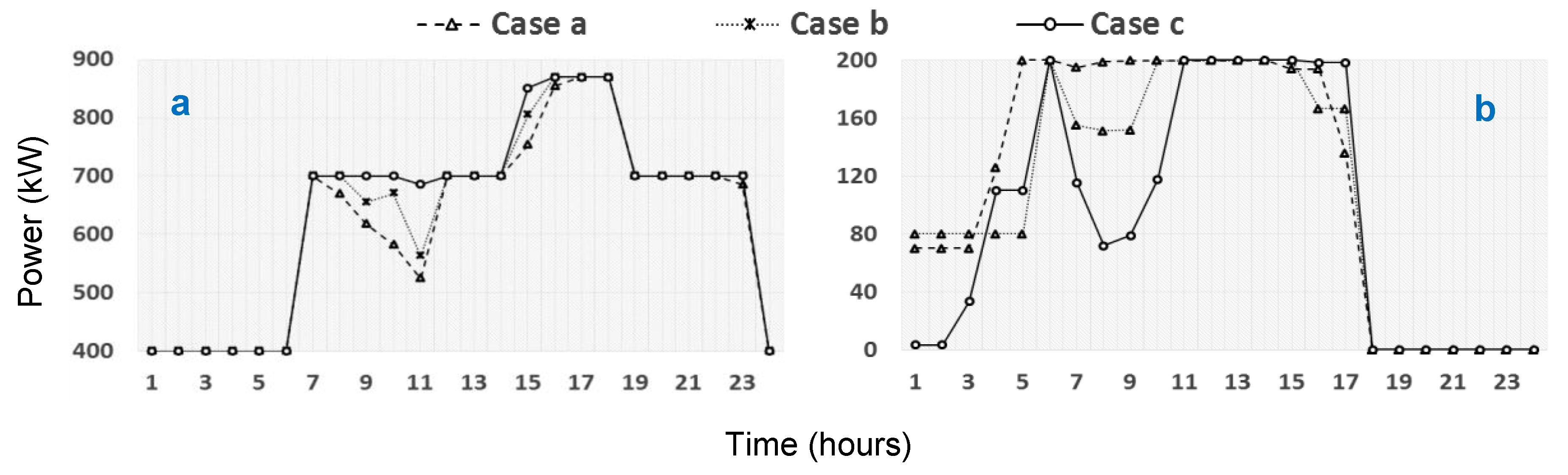
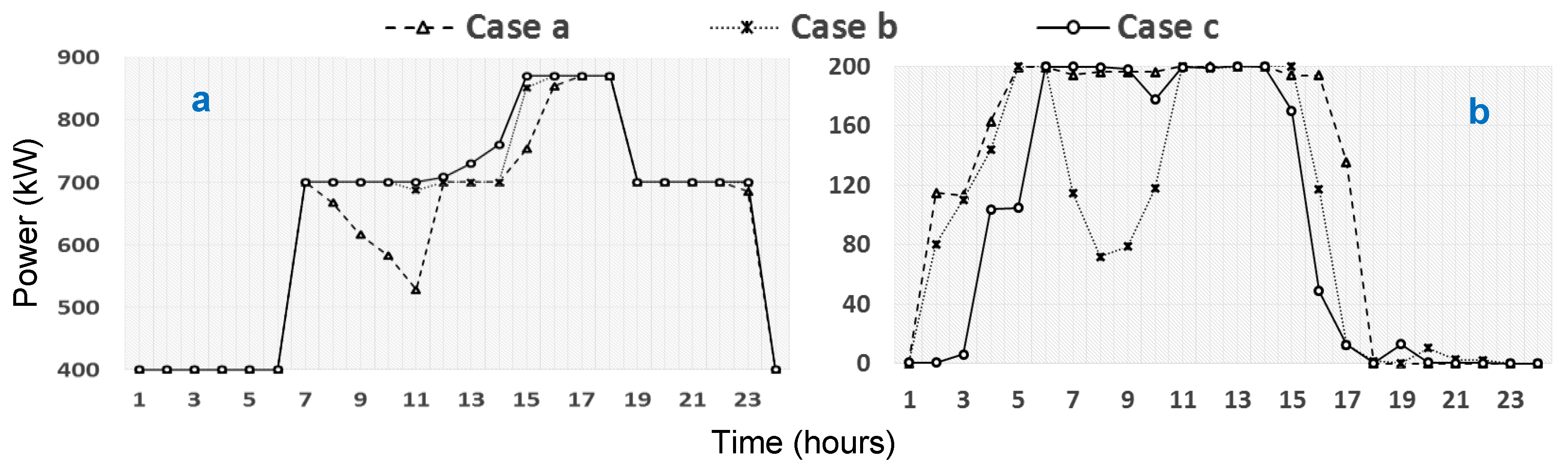
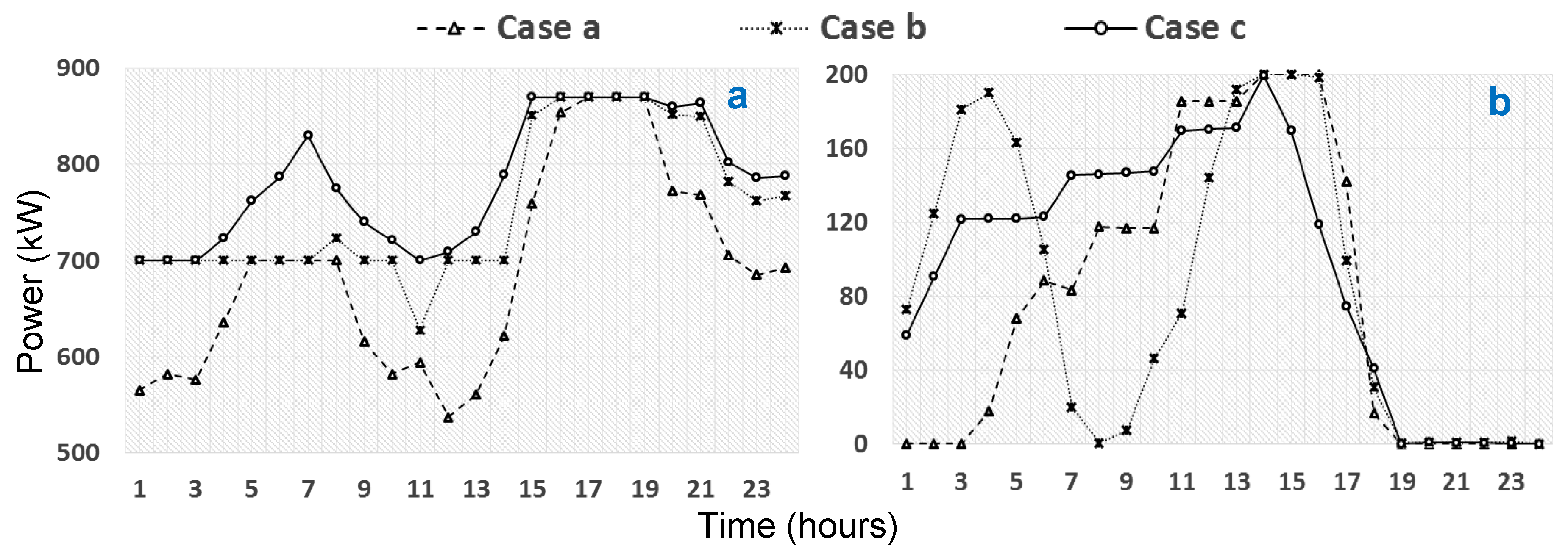
5.4.1. Grid-Connected Mode

Case b: The value of budget of uncertainty (${Г}_m\left(t\right)$) is set to one in this case which makes the optimization problem to select one of the two (load and renewable power) uncertainties at each time interval t. In order to assure the feasibility of solution under all possible realizations, instead of selecting randomly, the proposed algorithm has been set to select the worst value. Generally, due to higher magnitude of load as compared to renewable power generation, load uncertainty is higher and is selected by the optimization algorithm. However, in the time intervals 10–14 the uncertainty of renewable sources is at the peak and is higher than the uncertainty of load in the corresponding time intervals. Therefore, renewable power uncertainty has been considered by the RO algorithm in these time intervals and load uncertainty has been considered in the remaining time intervals.

The difference between Case a and Case b, as shown in Figure 11a, is identical to that of Case c in Section 5.3, as shown in Figure 9a, in the time intervals 1–6 and 24. The generation amounts of CGs in time intervals 7–11 and 19–23 are also identical to those of Case c in Figure 10a. However, the magnitude of reduction in selling power in time intervals 11–13 in Figure 11a is identical to that of Case c in Figure 7a. Behavior of BESS charging/discharging is similar to that of Figure 10b as shown in Figure 12b.

Case c: This is the worst possible case in the given framework of simulations. In this case, both of the random variables sets (load and renewable generators) are assumed to take their worst values in each time interval t. It can be observed from Figure 6a that the uncertainty gap is summation of Case c of Figure 5a and Case c of Figure 5b. Due to the absence of renewable energy sources (PV and CS) in the time intervals 1–7 and 19–24 the uncertainty gap adjustment trend is similar to that of Section 5.3. However, in the remaining time intervals due to combined uncertainties of both the random variable sets, the trend is different from other two cases explained in Section 5.2 and Section 5.3. Unlike to the other two cases, selling power has reduced to zero in time intervals 11–15, as shown in Figure 11a. Similarly, in both of the previous cases explained in Section 5.2 and Section 5.3 internal trading has been progressively increased from Case a to Case c, but Figure 11b shows that internal trading has decreased in Case c in comparison with Case b. This behavior is due to the fact that in Case c due to uncertainty in both of the random variable sets surplus amount of individual MGs has drastically reduced.

5.4.2. Islanded Mode

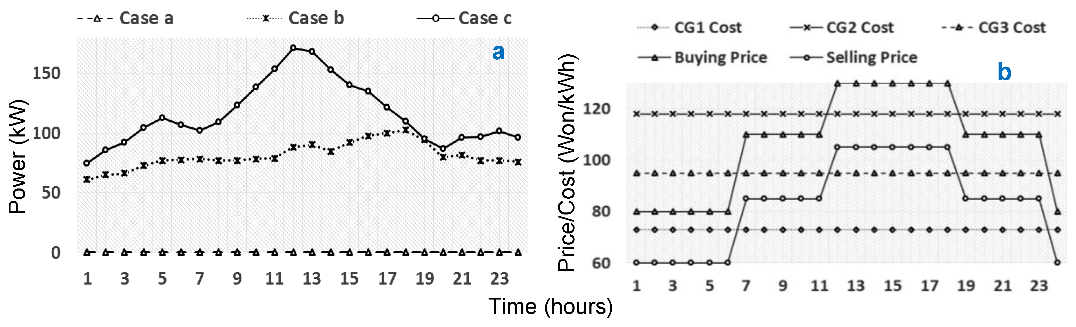
The objective of the islanded mode operation is to minimize both the operation cost and amount of load shedding. However, due to the finite capacities of power sources, load shedding might be unavoidable in some cases. It can be observed from Figure 13a that even for the deterministic case (${Г}_m\left(t\right)$ = 0), there is some unavoidable load shedding at time intervals 18 and 19. The generation amount of CGs shown in Figure 14a is different from the grid-connected case, i.e., Figure 12a. The case with SOC of BESSs is the same. BESSs have been used more efficiently in islanded mode to minimize the amount of load shedding.

Case b: In this case, one of the two uncertainties will be selected by the optimization algorithm and scheduling will be carried out for the worst case in the given frame of uncertainties. Amount of load shedding has been increased in this case as compared to the deterministic case. It can be observed from Figure 13a and 14b that load shedding has been carried out only in the peak load intervals after utilizing BESSs. The dynamics of BESSs charging/discharging are also changing more frequently as compared to the deterministic case.

Case c: In this case, both of the uncertainties (renewable power and load) have been considered by the optimization algorithm for scheduling of the MMG system. Amount of load shedding in the peak price intervals has further increased in this case. Due to the consideration of uncertainties in both renewable energy sources and electric loads, internal trading has been reduced in this case in comparison with previous cases. Figure 14a depicts that CGs outputs have been increased to fulfill the load demands. Load shedding has been carried out only in those time intervals where, both CGs and BESSs were unable to fulfill the electric load demands of the MMG system.

The general behavior in all the cases to minimize the operation cost and minimize the load shedding of the MMG system can be summarized as follows.

• When $PU{C}_{m,g}^{CG}\left(p_{m,g}^{CG}\left(t\right)\right)<C^{SELL}\left(t\right)$ <$C^{BUY}\left(t\right)$, CG generates to its fullest, sends to other MGs with CGs of higher cost, or sells to the utility grid.
• When $C^{SELL}\left(t\right)\le PU{C}_{m,g}^{CG}\left(p_{m,g}^{CG}\left(t\right)\right)$<$C^{BUY}\left(t\right)$, CG does not involve in external trading. It suffices its local load demands and may send to other MGs having expensive CGs.
• When$PU{C}_{m,g}^{CG}\left(p_{m,g}^{CG}\left(t\right)\right)\ge C^{BUY}\left(t\right)>C^{SELL}\left(t\right)$, CG generates minimum power and either receives from other MGs having cheaper CGs or buys from the utility grid.
• BESS is charged mainly in off-peak/mid-peak price intervals and discharged in the peak intervals.
• Internal trading is increased when BESS is discharged or generation of CGs in individual MGs is increased.
• Load shedding is carried out only in peak load intervals when both CGs and BESSs were unable to fulfill the electric load demands of the MMG system.

5.5. Operation Cost and Budget of Uncertainty

Various values of budget of uncertainty (${Г}_m\left(t\right)$) and probability of unfeasible solution (${\mathsf{\epsilon }}_e$) in the given uncertainty bounds have been compared against the daily operation cost of the MMG system in both operation modes. It can be observed from

Table 2. Performance in grid-connected mode with single source of uncertainty.

Budget of Uncertainty and Error			Uncertainty in Renewable Power		Uncertainty in Electric Load
${\mathbf{Г}}_{\mathit{m}}\left(\mathit{t}\right)$	${{\displaystyle \sum }}_{\mathit{t}=1}^{\mathit{T}}{\mathbf{Г}}_{\mathit{m}}\left(\mathit{t}\right)$	${\mathsf{\epsilon }}_{\mathit{e}}$	Cost (M ₩ 1)	Inc. (%age)	Cost (M ₩)	Inc. (%age)
0	0	0.58	1.53574	0	1.53574	0
0.25	6	0.15	1.55641	1.34	1.58472	3.10
0.5	12	0.012	1.57720	2.71	1.63419	6.42
0.75	18	2.6 × 10−4	1.59820	4.08	1.68384	9.66
1	24	1.3 × 10−6	1.61913	5.44	1.73342	12.89

¹ ₩ is Korean Won.

that operation cost for uncertain load is higher as compared to the corresponding uncertainty in renewable power, which is due to the absence of solar related renewable power in the morning and night times. Corresponding grid-connected mode operation cost has been used as a reference for calculating increase percentage in each case.

Table 3. Performance in islanded mode with single source of uncertainty.

Budget of Uncertainty and Error			Uncertainty in Renewable Power			Uncertainty in Electric Load
${\mathbf{Г}}_{\mathit{m}}\left(\mathit{t}\right)$	${{\displaystyle \sum }}_{\mathit{t}=\mathbf{1}}^{\mathit{T}}{\mathbf{Г}}_{\mathit{m}}\left(\mathit{t}\right)$	${\mathsf{\epsilon }}_{\mathit{e}}$	Shed Load (kWh)	Cost (M ₩ )	Inc. (%age)	Load Shed (kWh)	Cost (M ₩)	Inc. (%age)
0	0	0.58	66	1.57458	2.53	66	1.57458	2.53
0.25	6	0.15	74	1.59611	3.93	150	1.63200	6.27
0.5	12	0.012	84	1.61778	5.34	248	1.69128	10.13
0.75	18	2.6 × 10−4	100	1.64007	6.79	346	1.75064	13.99
1	24	1.3 × 10−6	117	1.66271	8.23	445	1.81058	17.90

shows that amount of load shedding increases with increase in the value of${Г}_m\left(t\right)$. The operation cost of the islanded mode is always greater than that of corresponding grid-connected mode. The two factors that result this increase are heavy penalty costs for shedding loads and inability of the MMG system to trade with the utility grid.

Table 4. Performance in both grid-connected and islanded modes with both uncertainty sources.

Budget of Uncertainty and Error			Grid-Connected Mode		Islanded Mode
${\mathbf{Г}}_{\mathit{m}}\left(\mathit{t}\right)$	${{\displaystyle \sum }}_{\mathit{t}=\mathbf{1}}^T{\mathbf{Г}}_{\mathit{m}}\left(\mathit{t}\right)$	${\mathsf{\epsilon }}_{\mathit{e}}$	Cost (M ₩)	Inc. (%age)	Shed Load (kWh)	Cost (M ₩)	Inc. (%age)
0	0	0.56	1.53574	0	66	1.57458	2.53
0.5	12	0.056	1.63504	6.07	248	1.69200	10.16
1	24	4.5 × 10−4	1.73501	12.98	446	1.81187	17.98
1.5	36	2.2 × 10−6	1.77778	15.76	484	1.86143	21.21
2	48	5.8 × 10−12	1.82185	18.63	541	1.91449	24.66

shows the operation cost considering uncertainties in both renewable power sources and loads. It can be observed that the operation cost at ${Г}_m\left(t\right)$ = 1 is higher than both of the operation cost in Table 1 at ${Г}_m\left(t\right)$ = 1 which is due to the consideration of worst scenario. The case with amount of load shedding is the same. However, probability of error has increased at ${Г}_m\left(t\right)$= 1 due to inclusion of more random variables.

6. Conclusions

An RO-based algorithm has been proposed for day-ahead scheduling of multi-microgrids in grid-connected mode. Instead of using a hard-to-obtain probability distribution of the uncertain data, a deterministic uncertainty set (upper and lower bounds) has been used in this formulation. Simulation results have proved that the developed MILP-based model is capable of providing guaranteed immunity in contrast to probabilistic guarantee of stochastic optimization techniques against the worst-case scenario: maximum uncertainty in both renewable power source and load. The developed model can be easily implemented using commercial optimization tools and it remains tractable even for large systems. The behavior of the simulation results shows that the objective of the proposed strategy is to reduce the operation cost of the MMG system in grid-connected mode and minimize load shedding while reducing operation cost in islanded mode. The unit commitment status of CGs and BESSs determined in each case remains valid even if the load and/or renewable power outputs fluctuate with the determined bounds of uncertainties. It can be concluded form the simulation results that the probability of unfeasible solution reduces drastically as the budget of uncertainty increases. Therefore, a trade-off can easily be obtained by the decision makers. The increase in operation cost in islanded mode is due to penalties for load shedding and inability of the MMG system to trade with utility grid. Simulation results depict the required units of power sources to be committed, in order to assure the proper operation of MMG system under the given uncertainty.

References

1. Liu, G.; Xu, Y.; Tomsovic, K. Bidding strategy for microgrid in day-ahead market based on hybrid stochastic/robust optimization. IEEE Trans. Smart Grid 2016, 7, 227–237. [Google Scholar] [CrossRef]
2. Bertsimas, D.; Litvinov, E.; Sun, X.A.; Zhao, J.; Zheng, T. Adaptive robust optimization for the security constrained unit commitment problem. IEEE Trans. Power Syst. 2013, 28, 52–63. [Google Scholar] [CrossRef]
3. Li, H.; Guo, S.; Zhao, H.; Su, C.; Wang, B. Annual electric load forecasting by a least squares support vector machine with a fruit fly optimization algorithm. Energies 2012, 5, 4430–4445. [Google Scholar] [CrossRef]
4. Papaioannou, D.I.; Papadimitriou, C.N.; Dimeas, A.L.; Zountouridou, E.I.; Kiokes, G.C.; Hatziargyriou, N.D. Optimization & Sensitivity Analysis of Microgrids using HOMER Software—A Case Study. In Proceedings of the IEEE Mediterranean Conference on Power Generation, Transmission, Distribution and Energy Conversion, Athens, Greece, 2–5 November 2014.
5. Chang, W.Y. Short-term wind power forecasting using the enhanced particle swarm optimization based hybrid method. Energies 2013, 6, 4879–4896. [Google Scholar] [CrossRef]
6. Feng, J.; Shen, W.Z. Modelling wind for wind farm layout optimization using joint distribution of wind speed and wind direction. Energies 2015, 8, 3075–3092. [Google Scholar] [CrossRef] [Green Version]
7. Lin, W.M.; Tu, C.S.; Tsai, M.T. Energy management strategy for microgrids by using enhanced bee colony optimization. Energies 2016, 9. [Google Scholar] [CrossRef]
8. Sperati, S.; Alessandrini, S.; Pinson, P.; Kariniotakis, G. The “weather intelligence for renewable energies” benchmarking exercise on short-term forecasting of wind and solar power generation. Energies 2015, 8, 9594–9619. [Google Scholar] [CrossRef] [Green Version]
9. Lorca, A.; Sun, X.A. Adaptive robust optimization with dynamic uncertainty sets for multi-period economic dispatch under significant wind. IEEE Trans. Power Syst. 2015, 30, 1702–1713. [Google Scholar] [CrossRef]
10. Simmhan, Y.; Prasanna, V.; Aman, S.; Natarajan, S.; Yin, W.; Zhou, Q. Demo abstract: Toward data-driven demand-response optimization in a campus microgrid. In Proceedings of the ACM Workshop on Embedded Sensing Systems For Energy-Efficiency in Buildings, Seattle, WA, USA, 1–4 November 2011.
11. Liu, Y.K. Convergent results about the use of fuzzy simulation in fuzzy optimization problems. IEEE Trans. Fuzzy Syst. 2006, 14, 295–304. [Google Scholar] [CrossRef]
12. Liang, H.; Zhuang, W. Stochastic modeling and optimization in a microgrid: A survey. Energies 2013, 7, 2027–2050. [Google Scholar] [CrossRef]
13. Wang, R.; Wang, P.; Xiao, G. A robust optimization approach for energy generation scheduling in microgrids. Energy Convers. Manag. 2015, 106, 597–607. [Google Scholar] [CrossRef]
14. Jiang, R.; Wang, J.; Guan, Y. Robust unit commitment with wind power and pumped storage hydro. IEEE Trans. Power Syst. 2012, 27, 800–810. [Google Scholar] [CrossRef]
15. Akbari, K.; Nasiri, M.M.; Jolai, F.; Ghaderi, S.F. Optimal investment and unit sizing of distributed energy systems under uncertainty: A robust optimization approach. Energy Build. 2014, 85, 275–286. [Google Scholar] [CrossRef]
16. Kuznetsova, E.; Li, Y.F.; Ruiz, C.; Zio, E. An integrated framework of agent-based modeling and robust optimization for microgrid energy management. Appl. Energy 2014, 129, 70–88. [Google Scholar] [CrossRef]
17. Peng, C.; Xie, P.; Pan, L.; Yu, R. Flexible robust optimization dispatch for hybrid wind/ photovoltaic/ hydro/thermal power system. IEEE Trans. Smart Grid 2016, 7, 751–762. [Google Scholar] [CrossRef]
18. Rezvan, A.T.; Gharneh, N.S.; Gharehpetian, G.B. Robust optimization of distributed generation investment in buildings. Energy 2012, 48, 455–463. [Google Scholar] [CrossRef]
19. Jabr, R.A. Robust transmission network expansion planning with uncertain renewable generation and loads. IEEE Trans. Power Syst. 2013, 28, 4558–4567. [Google Scholar] [CrossRef]
20. Wang, Z.; Chen, B.; Wang, J.; Kim, J.; Begovic, M.M. Robust optimization based optimal DG placement in microgrids. IEEE Trans. Smart Grid 2014, 5, 2173–2182. [Google Scholar] [CrossRef]
21. Hajimiragha, A.H.; Canizares, C.A.; Fowler, M.W.; Moazeni, S.; Elkamel, A. A robust optimization approach for planning the transition to plug-in hybrid electric vehicles. IEEE Trans. Power Syst. 2011, 26, 2264–2274. [Google Scholar] [CrossRef]
22. Kim, S.J.; Giannakis, G. Scalable and robust demand response with mixed-integer constraints. IEEE Trans. Smart Grid 2013, 4, 2089–2099. [Google Scholar] [CrossRef]
23. Salomon, S.; Avigad, G.; Fleming, P.J.; Purshouse, R.C. Active robust optimization: enhancing robustness to uncertain environments. IEEE Trans. Cybernet. 2014, 44, 2221–2231. [Google Scholar] [CrossRef] [PubMed]
24. Olivares, D.E.; Claudio, A.C.; Mehrdad, K. A centralized optimal energy management system for microgrids. In Proceedings of the IEEE Power and Energy Society General Meeting, San Diego, CA, USA, 24–29 July 2011; pp. 1–6.
25. Song, N.O.; Lee, J.H.; Kim, H.M.; Im, Y.H.; Lee, J.Y. Optimal energy management of multi-microgrids with sequentially coordinated operations. Energies 2015, 8, 8371–8390. [Google Scholar] [CrossRef]
26. Wang, Y.; Shiwen, M.; Nelms, R.M. On hierarchical power scheduling for the macrogrid and cooperative microgrids. IEEE Trans. Ind. Inform. 2015, 11, 1574–1584. [Google Scholar] [CrossRef]
27. Shi, W.; Xie, X.; Chu, C.C.; Gadh, R. Distributed optimal energy management in microgrids. IEEE Trans. Smart Grid 2015, 6, 1137–1146. [Google Scholar] [CrossRef]
28. Kim, H.M.; Kinoshita, T.; Shin, M.C. A multiagent system for autonomous operation of islanded microgrids based on a power market environment. Energies 2010, 3, 1972–1990. [Google Scholar] [CrossRef]
29. Tian, P.; Wang, X.; Wang, K.; Ding, R. A hierarchical energy management system based on hierarchical optimization for microgrid community economic operation. IEEE Trans. Smart Grid 2015. [Google Scholar] [CrossRef]
30. Nguyen, D.T.; Le, L.B. Optimal energy management for cooperative microgrids with renewable energy resources. In Proceedings of the IEEE International Conference on Smart Grid Communications, Vancouver, BC, Canada, 21–24 October 2013. [CrossRef]
31. Alharbi, W.; Raahemifar, K. Probabilistic coordination of microgrid energy resources operation considering uncertainties. Elect. Power Syst. Res. 2015, 128, 1–10. [Google Scholar] [CrossRef]
32. Liang, R.H.; Liao, J.H. A fuzzy-optimization approach for generation scheduling with wind and solar energy systems. IEEE Trans. Power Syst. 2007, 22, 1665–1674. [Google Scholar] [CrossRef]
33. Ben-Tal, A.; Goryashko, A.; Guslitzer, E.; Nemirovski, A. Adjustable robust solutions of uncertain linear programs. Math. Prog. 2004, 99, 351–376. [Google Scholar] [CrossRef]
34. Jiang, R.; Zhang, M.; Li, G. Two-Stage Robust Power Grid Optimization Problem. Available online: http://www.optimization-online.org/DBFILE/2010/10/2769.pdf (accessed on 07 April 2016).
35. Bertsimas, D.; Sim, M. The price of robustness. Oper. Res. 2004, 52, 35–53. [Google Scholar] [CrossRef]
36. Xiang, Y.; Liu, J.; Liu, Y. Robust energy management of microgrid with uncertain renewable generation and load. IEEE Trans. Smart Grid 2016, 7, 1034–1043. [Google Scholar] [CrossRef]
37. Khosravi, A.; Nahavandi, S.; Creighton, D.; Atiya, A.F. Lower upper bound estimation method for construction of neural network-based prediction intervals. IEEE Trans. Neur. Netw. 2011, 22, 337–346. [Google Scholar] [CrossRef] [PubMed]
38. Khosravi, A.; Nahavandi, S.; Creighton, D. Construction of optimal prediction intervals for load forecasting problems. IEEE Trans. Power Syst. 2010, 25, 1496–1503. [Google Scholar] [CrossRef]
39. Bidram, A.; Ali, D. Hierarchical structure of microgrids control system. IEEE Trans. Smart Grid 2012, 3, 1963–1976. [Google Scholar] [CrossRef]
40. Liu, P. Stochastic and Robust Optimal Operation of Energy-Efficient Building with Combined Heat and Power Systems. Ph.D. Thesis, Mississippi State University, Mississippi State, MS, USA. Available online: http://search.proquest.com/docview/1640887456 (accessed on 19 February 2016).
41. Khodaei, A.; Shay, B.; Mohammad, S. Microgrid planning under uncertainty. IEEE Trans. Power Syst. 2015, 30, 2417–2425. [Google Scholar] [CrossRef]
Figure 1. Uncertainty representation: (a) Deterministic optimization; (b) Stochastic optimization; and (c) Robust optimization.
Energies 09 00278 g001
Figure 2. Problem formulation process of robust optimization.
Energies 09 00278 g002
Figure 3. An illustration of a typical multi-microgrid system.
Energies 09 00278 g003
Figure 4. (a) Hourly electric load of microgrids (MGs); and (b) Hourly renewable generation outputs in each microgrid (MG).
Energies 09 00278 g004
Figure 5. Hourly collective uncertainty gap: (a) Renewable energy sources; and (b) Electric loads.
Energies 09 00278 g005
Figure 6. (a) Hourly collective uncertainty gap for both renewable power sources and electric loads; and (b) Market price signals along with generation cost of controllable distributed generators.
Energies 09 00278 g006
Figure 7. Collective power trading: (a) Internal trading; and (b) External trading.
Energies 09 00278 g007
Figure 8. (a) Collective generation amount of Controllable generators (CGs); and (b) Cumulative state of charge (SOC) of battery energy storage system (BESSs).
Energies 09 00278 g008
Figure 9. Collective power trading: (a) Internal trading; and (b) External trading.
Energies 09 00278 g009
Figure 10. (a) Collective generation amount of CGs; and (b) Cumulative SOC of BESSs.
Energies 09 00278 g010
Figure 11. Collective power trading in grid connected mode: (a) Internal trading; and (b) External trading.
Energies 09 00278 g011
Figure 12. Grid-connected mode: (a) Collective generation amount of CGs; and (b) Cumulative SOC of BESSs.
Energies 09 00278 g012
Figure 13. Islanded mode: (a) Collective amount of load shed; and (b) Internal trading.
Energies 09 00278 g013
Figure 14. Islanded mode: (a) Collective generation amount of CGs; and (b) Cumulative SOC of BESSs.
Energies 09 00278 g014