Forecasting the Allocative Efficiency of Carbon Emission Allowance Financial Assets in China at the Provincial Level in 2020

Abstract

As the result of climate change and deteriorating global environmental quality, nations are under pressure to reduce their emissions of greenhouse gases per unit of GDP. China has announced that it is aiming not only to reduce carbon emission per unit of GDP, but also to consume increased amounts of non-fossil energy. The carbon emission allowance is a new type of financial asset in each Chinese province and city that also affects individual firms. This paper attempts to examine the allocative efficiency of carbon emission reduction and non-fossil energy consumption by employing a zero sum gains data envelopment analysis (ZSG-DEA) model, given the premise of fixed CO₂ emissions as well as non-fossil energy consumption. In making its forecasts, the paper optimizes allocative efficiency in 2020 using 2010 economic and carbon emission data from 30 provinces and cities across China as its baseline. An efficient allocation scheme is achieved for all the provinces and cities using the ZSG-DEA model through five iterative calculations.

1. Introduction

The carbon emission allowance is a new type of financial asset. This article addresses the new type of financial asset allocative efficiency in each Chinese province and city, which we define as the mix of carbon emission reductions and increases across provinces and cities that must be calculated to achieve reach efficient frontiers. In other words, the most efficient region is that with the lowest energy consumption and CO₂ emission levels but with the same GDP and population values that it had with no environmental constraints. As an accompaniment to China’s rapid economic growth, greenhouse gas emissions have caused serious pollution that has negatively affected the nation’s ecology and marginalized its natural environment. As a result, China is facing critical problems that must be solved, and studies of carbon emission resulting from energy consumption focus on questions involving how to achieve reasonable emission reductions while balancing the relationship between economic development and environmental concerns. China’s government has committed to reducing its carbon emission per unit of GDP by 40%–50% during the 2005–2020 period. During this same period, non-fossil energy consumption is targeted to account for 15% of total primary energy consumption. Non-fossil energy includes wind-generated energy, water-generated energy, nuclear energy, and solar power. The purpose of these reduction targets is to limit overall emissions and achieve positive environmental effects. Although the national target for overall emissions has been set, the key problem that remains is how to apportion the total target effectively, fairly, justly and reasonably among China’s provinces and cities in the face of the huge disparities in economic development, energy structures and CO₂ emissions and emission schemes that characterizes the different regions. Thus, taking the appropriate related factors into account to achieve allocative efficiency and to maximize effectiveness is a formidable task for China. As of 14 December 2015, seven provinces and cities in China—Shenzhen, Shanghai, Beijing, Guangdong, Tianjin, Chongqing and Hubei—initiated carbon emissions trading schemes. Nonetheless, it is important to know how to allocate carbon allowances to make trading them effective and efficient in China’s 30 provinces and cities.

2. Literature Review

2.1. Carbon Allowance Allocation

A carbon allowance trading scheme attempts to solve environmental problems by using market forces to more effectively allocate resources and to eliminate negative externalities. However, the calculations involved in allocating the initial rights for carbon emissions are pivotal in their impact on transactional efficiency. Therefore, further studies of allocating carbon allowances are both necessary and productive.

From the perspective of government policies, Ding and Feng [1] considered both domestic and international factors in their evaluation of the different modes of carbon allowance allocation and the policy implications associated with each. These authors proposed that China should set up a free allocation mode based on historical data at an early stage but that a paid auction-based mode should be established at a later stage. Sun and Ma [2] compared the advantages and disadvantages of existing initial allocation methods and analysed the current main carbon emission trading schemes that have been implemented all over the world. Based on the results of their research, these authors suggested that a fixed proportion of the free carbon emission allowance should be assigned when a trading scheme is initially established and that it should be further transformed stage-by-stage to gradually reduce the proportion of free allowances until trading is conducted exclusively on an auction basis.

In terms of the allocation modes of carbon emissions, Yin and Cui [3] proposed an allocation scheme based on GDP per capita and energy consumption per GDP. Moreover, Wang Yigang [4] justified a flexible allocation scheme based on ensuring development rights.

With regard to research approaches to allocating carbon allowances, Jiang Jingjing [5] developed a mechanism (and an experiment) for carbon allowance allocation in the Shenzhen manufacturing sector by analyzing the grandfathering allocation mode of Europe’s carbon trading scheme—using the condition of incomplete information as its theoretical basis—and by applying limited rational assumptions and repeated game theories. Cong Ronggang [6] suggested a multi-agent carbon allocation auction model (CAAM) based on the auction mechanism of the EU’s carbon market and investigated whether the clearing auction price should take the form of uniform pricing or discriminatory pricing. Wang and Li [7] proposed a new data envelopment analysis carbon emissions allocation (DEA-CEA) model on the basis of data envelopment analysis (DEA) methodology. These authors considered the issue of CO₂ emissions distribution to be a resource allocation problem in which the total amount is controlled and regarded efficiency as a priority and the per capita amount as a restraint when allocating national total emissions to each province.

To conclude, although there are significant differences in carbon allowance schemes among different countries, there are lessons that these countries can learn from one another. Additionally, allocation benchmarks and research methods vary from country to country based on countries’ specific conditions. In general, China is considered to be in the primary stages of establishing a carbon allowance system, although its conditions differ from those of other countries. Therefore, further studies are required to establish a suitable and efficient carbon allowance system in China.

2.2. Carbon Allowance Allocation Based on Efficiency

The first and most prominent system for regulating carbon emissions is the European Union Emissions Trading Scheme (EU ETS). We examine the effectiveness of the EU ETS in terms of a cap-and-trade system. When it was first established, its efficiency was studied on the macro level. Rogge and Hoffmann [8] believed that the impact of the EU ETS on corporate CO₂ culture and routines would pave the way for a transition to a low-carbon innovation system for power generation technologies. Sandoff and Schaad [9] conducted a survey and found that although Swedish companies have shown significant interest in reducing emissions, these companies have not paid close attention to the pricing mechanism of market-based instruments. If this praxis is widespread within the European trading sector, it might seriously and negatively impact system efficiency. Zhang and Wei [10] found that previous research results do not indicate that the EU ETS has had significant economic effects on energy technology investment. The enterprise competitiveness loss caused by the EU ETS has not been strong, but it may become stronger in the future. In later studies, efficiency was studied at the micro level. Moreover, different streams in the literature found that the macro-distribution of carbon allowance assets and EU CO₂ allowance price volatility exerted different effects on the stock market. Oestreich and Tsiakas [11] found that on average, firms that received free carbon emission allowances under the EU ETS significantly outperformed firms that did not, as measured by German stock returns. There was no significant value impact from firms' allowance trading activity or from the pass-through of carbon-related production costs (carbon leakage) [12]. While firms reduced their environmental costs, stock prices also fell for firms in both carbon- and electricity-intensive industries within the EU when the EU CO₂ allowance price dropped 50 per cent in late April 2006 [13].

Most efficiency studies are conducted by employing a variety of input-output models, which leads to the problem of assessing the efficiencies of multiple inputs and outputs of the same types of decision-making units (DMUs), which is why the DEA model is widely used in this context [14]. In comparison with traditional DEA models that presume that output is the expected output (i.e., the larger the output is, the more effective the decision unit is), carbon emissions are regarded as non-expected output, i.e., the smaller the output, the more effective the decision unit is. The DEA model with non-expected output is commonly used in the analysis of environmental efficiency. Zofio and Prieto [15] evaluated environmental efficiency among Organization for Economic Co-operation and Development (OECD) countries by taking carbon dioxide emissions as the non-expected output. Lozano and Gutierrez [16] examined the correlations between GDP, carbon emissions and energy consumption with the distance function method of the DEA model by taking both carbon emissions and energy consumption as the non-expected output.

The non-expected output is independent of DMUs, and each decision unit is also independent of the other decision units. However, with regard to the rights allocations of carbon emissions, the amount of emissions between each decision unit is dependent because there is a fixed amount of available emission rights, i.e., it is a zero sum game (ZSG). When a unit increases or reduces its carbon emissions to achieve greater efficiency, the other DMUs must correspondingly decrease or increase the same amount of carbon emissions to maintain the ZSG.

Lins and Gomes et al. [17] proposed a zero sum gains data envelopment analysis (ZSG-DEA) model to adjust to non-expected output based on the DEA efficiency value of the DMU. Lin and Ning [18] assessed the allocation outcomes of EU countries’ carbon emission rights in 2009 based on a ZSG-DEA model. Sun Zuoren et al. [19] investigated the weak disposability of non-expected output and the restraint conditions of the total amount of energy consumption by employing the ZSG-DEA model. The results were used to formulate the allocation of energy efficiency index of the “12th Five Year Plan” in China. Wu et al. [20] studied the allocative efficiency of PM2.5 emission rights based on a zero sum gains DEA model. Pang et al. [21] studied the reallocation of carbon emission allowance with regard to all the countries participating in the Kyoto Protocol. Wang et al. [22] investigated the regional allocation of CO₂ emissions allowance among Chinese provinces, whereas Miao et al. [23] investigated the efficient allocation of CO₂ emissions in China.

This paper differs from those of Wang et al. [22] and Miao et al. [23] by focussing its investigation on the allocation of the CO₂ emissions allowance among China’s provinces based on China’s real 2010 carbon emission data, which is used as a benchmark. This paper is also distinguished from references [24,25,26,27,28,29,30,31,32,33,34,35,36], which did not use the ZSG-DEA model and/or did not research the CO₂ emissions allowance among China’s provinces. Instead, this paper attempts to measure the expected efficiency of carbon emissions allocation in 2020 in China by employing the ZSG-DEA model and further investigates how to establish an efficient allocation under the conditions of fixed total carbon emission rights based on the calculated parameter results.

The contribution of this paper to policy making is as follows: policy makers should adjust the distribution of carbon allowance to achieve the multiple goals of carbon emission reduction and non-fossil energy consumption in different areas in China. Simultaneously, fairness can be achieved among all provinces and cities at the new ZSG-DEA frontier by consider GDP and population (POP) as factors.

3. Empirical Results and Discussion

DEAP2.1 software and an Excel planning method were used to solve the original DEA and ZSG-DEA efficiency. The last column of

Table 1. Predicted statistics and efficiency values in 2020 by taking 2010 as the benchmark. Data envelopment analysis: DEA.

Region	GDP *	POP **	TEC ***	CDE ****	NFEC *****	Initial DEA Efficiency
Beijing	26,877.87	2068.83	22,419.36	9139.91	1367.02	1.000
Tianjin	18,004.03	1485.04	20,914.45	9121.63	2889.98	0.709
Hebei	36,199.64	7656.45	96,631.92	44,090.88	10,385.22	0.519
Shanxi	12,449.74	3716.95	65,261.87	39,113.35	10,956.98	0.250
Inner Mongolia	25,285.27	2614.88	80,577.81	26,620.04	12,531.91	0.467
Liaoning	35,699.68	4689.23	82,569.12	36,992.38	6424.49	0.554
Jilin	18,129.91	2944.26	29,774.55	13,487.87	3248.63	0.628
Heilongjiang	15,782.96	4091.55	40,554.55	18,324.52	3825.59	0.730
Shanghai	30,934.54	2170.85	33,221.39	16,012.34	4896.33	0.683
Jiangsu	80,671.03	8447.49	90,921.19	35754.88	17,178.75	0.800
Zhejiang	47,522.26	5760.86	64,437.20	23,966.21	11,986.14	0.732
Anhui	25,379.27	6557.59	47,523.72	15,409.76	7412.07	0.793
Fujian	30,288.19	3945.73	36,315.67	10,800.30	7006.64	1.000
Jiangxi	17,176.17	4828.64	19,895.95	8897.53	3316.20	1.000
Shandong	75,516.20	10,288.25	142,845.79	55,889.96	15,926.08	0.559
Henan	41,507.36	10,215.61	73,841.23	33,116.81	11,424.78	0.635
Hubei	33,409.65	6117.83	43,513.36	18,272.22	10,483.98	0.728
Hunan	32,288.39	6904.05	36,930.61	16,870.52	5738.38	0.872
Guangdong	82,065.21	10,649.49	82,889.85	31,925.15	14,533.07	0.933
Guangxi	17,782.83	5342.28	21,211.93	8176.29	5369.34	1.000
Hainan	3738.86	951.63	19,054.95	2322.30	717.30	1.000
Chongqing	15,993.10	3101.11	23,959.36	7601.55	2562.52	0.936
Sichuan	34,233.93	8723.45	54,657.75	17,616.22	8862.26	0.904
Guizhou	8790.90	4109.35	28,160.29	13,197.12	6845.51	0.544
Yunnan	13,257.43	4976.77	29,012.71	13,031.79	7063.82	0.646
Shanxi	19,403.74	4068.94	43,617.41	15,249.49	4979.50	0.618
Gansu	6970.92	2847.05	21,029.52	9459.62	4438.93	0.547
Qinghai	2169.99	606.41	6678.64	2178.34	2453.37	0.537
Ningxia	3284.43	691.15	15,651.77	5856.23	2941.96	0.336
Xinjiang	7614.99	2428.29	32,695.00	12,639.81	3248.63	0.533
Total	818,427.83	143,000.00	1,406,769.35	571,135.03	211,015.40	0.731 ******

* Unit: 100 million Chinese Yuan; ** Population (unit: 10 thousand Chinese Yuan); *** Total energy consumption (unit: 10 thousand tce, where tce is tons of standard coal, the unified standard unit of heat value); **** CO₂ emissions (unit: 10 thousand t.c., where t.c. is tons of carbon, the standard unit of CO₂ emissions); ***** Non-fossil energy consumption (unit: 10 thousand tce); ****** It is the average initial distribution efficiencyof provinces and cities.

presents the results of the original DEA efficiency for 2020, which reveals that the average initial distribution efficiency is 0.731, i.e., a medium-level average efficiency, and that the differences between provinces and cities are dramatic. Table 1 indicates that the efficiency values of 15 provinces are under average levels, which accounts for 50 per cent of these values. Furthermore, the initial efficiency values for five provinces and cities reach 1, which demonstrates that the allocation for these five provinces and cities is DEA effective but that the other 25 provinces and cities are not DEA efficient. Some provinces, such as Shan Xi and Ning Xia, do not perform well in terms of efficiency. For provinces with abundant energy resources, such as Shan Xi, a low efficiency value means that there is greater potential to reduce carbon emissions.

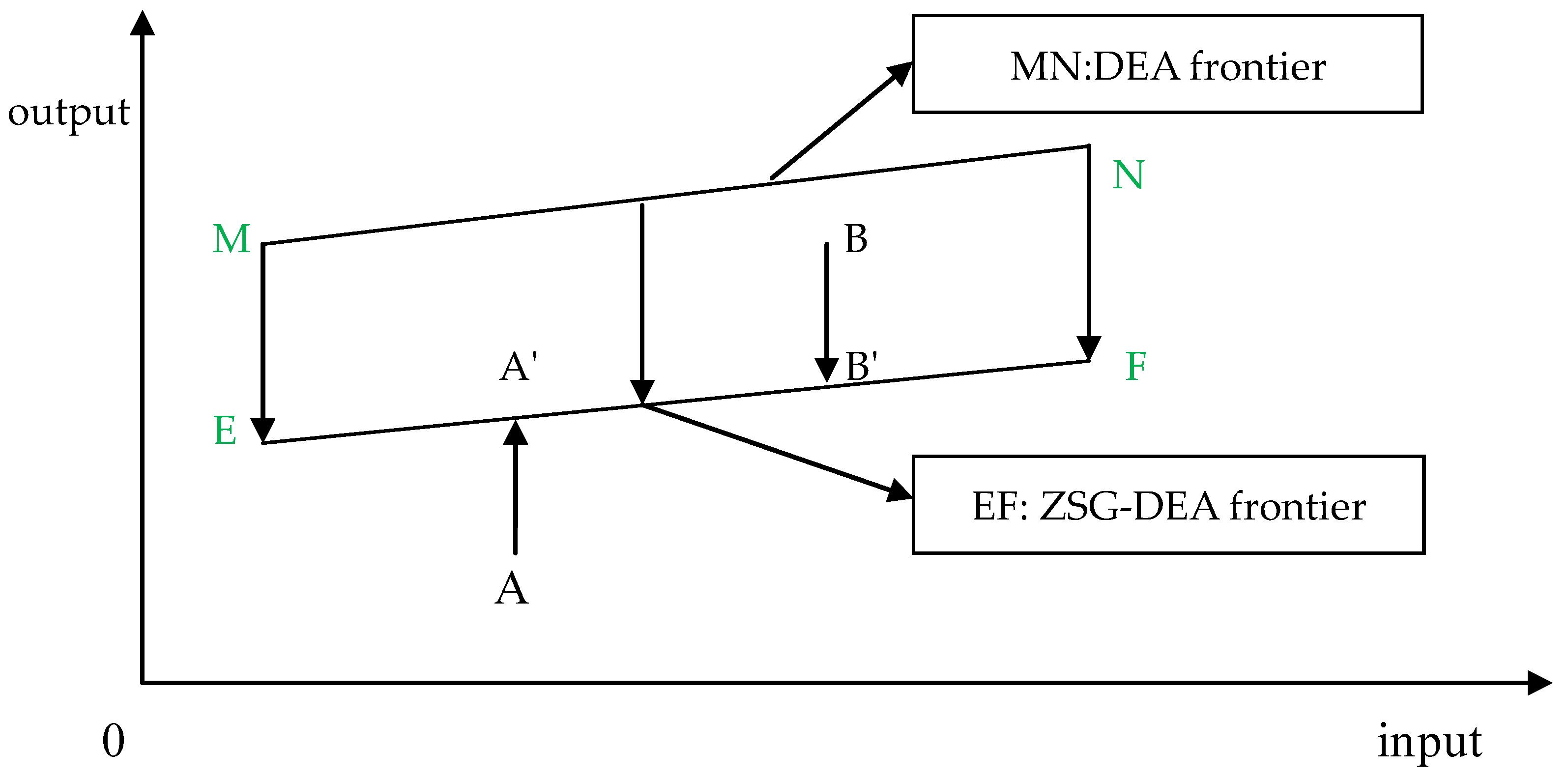
Based on the original DEA model, we may adjust the emission rights of all provinces and cities based on their efficiency values and slack variables so that the lowest carbon emission with respect to the economy and the carbon dioxide emission with the greatest efficiency might be achieved. However, this adjustment does not consider specific allocation situations, which is not feasible. For example, the total amount of carbon dioxide emission is fixed, which means that when one DMU reduces the input of a variable, the input of this variable into another DMU will increase accordingly. The efficiency values of original DEA and slack variables are not consistent with restraining the fixed total amount and are not able to achieve reasonable reallocation of input. Therefore, we must assess the efficiency values of the ZSG-DEA model and make proper adjustments of carbon emission rights based on the efficiency values and slack variables of the ZSG-DEA model.

Fair and effective allocation results in effective allocative efficiencies for all participating provinces, whether in the original DEA model or in the ZSG-DEA model. As discussed above, the status quo of most provinces and cities is currently ineffective, and for that reason we must adjust the ZSG-DEA model. Based on Equation (2), the amount that carbon emission must be reduced in some areas and the amount of increase needed in other provinces and cities can be calculated to reach the efficient frontiers. The multiple iteration method is employed to allow all provinces and cities reach their efficient frontiers.

According to the results of the ZSG-DEA model in the initial allocation, we obtain the voluntary trade matrix for all provinces and cities, and the results of the adjusted allocation are shown in

Table A1. Multiple iterations of data and DEA efficiency values of the first iteration.

Province	CO2 * (10 Thousand t.c. **)	NFF *** (10 Thousand tce ****)	DEA Efficiency Value
Beijing	12,532.24	2119.32	1.000
Tianjin	9854.37	2676.44	0.906
Hebei	30,763.29	9312.45	0.906
Shanxi	21,009.38	8344.09	0.567
Inner Mongolia	21,712.03	9564.39	0.791
Liaoning	27,870.89	7007.52	0.788
Jilin	10,915.47	3866.11	0.982
Heilongjiang	15,077.71	4994.13	0.893
Shanghai	16,807.32	4440.14	0.898
Jiangsu	42,785.85	14,348.55	0.952
Zhejiang	27,337.58	10,088.93	0.923
Anhui	18,907.47	8556.65	0.951
Fujian	16,007.48	6409.96	1.000
Jiangxi	12,199.89	5141.15	1.000
Shandong	50,029.84	15,332.91	0.867
Henan	32,678.81	13,164.68	0.883
Hubei	21,436.20	9654.66	0.927
Hunan	21,128.66	7863.01	0.966
Guangdong	43,772.33	14,682.08	0.989
Guangxi	12,902.90	6579.39	1.000
Hainan	3184.24	1112.04	1.000
Chongqing	10,128.85	3554.47	0.987
Sichuan	24,003.86	10,807.61	0.989
Guizhou	12,769.24	6503.37	0.831
Yunnan	14,244.31	7216.05	0.882
Shaanxi	16,103.73	5712.56	0.814
Gansu	9041.52	4384.72	0.823
Qinghai	1974.81	1870.26	0.867
Ningxia	4101.65	2179.96	0.658
Xinjiang	9853.11	3527.80	0.773

* CO₂ emission; ** t.c., tons of carbon (the standard unit of CO₂ emission); *** non-fossil fuel; **** tce, tons of standard coal (the unified standard unit of heat value).

,

Table A2. Multiple iterations of data and DEA efficiency values of the second iteration.

Province	CO2* (10 Thousand t.c. **)	NFF *** (10 Thousand tce ****)	DEA Efficiency Value
Beijing	13,979.17	2694.60	1.000
Tianjin	10,049.35	2436.27	0.975
Hebei	25,989.19	9345.60	1.000
Shanxi	14,045.30	6381.48	0.950
Inner Mongolia	19,495.64	7425.92	0.952
Liaoning	24,305.74	7373.26	0.976
Jilin	9558.30	4287.97	1.000
Heilongjiang	13,442.03	5848.76	0.963
Shanghai	16,983.06	3990.04	0.975
Jiangsu	45,971.28	12,411.58	0.930
Zhejiang	28,674.44	8704.35	0.908
Anhui	20,322.63	9362.81	0.970
Fujian	18,281.37	5859.27	0.915
Jiangxi	13,608.45	6536.71	1.000
Shandong	48,896.29	15,122.64	0.946
Henan	32,513.92	14,476.35	0.950
Hubei	22,680.89	9002.52	0.904
Hunan	22,880.20	9452.04	0.960
Guangdong	48,825.56	14,925.97	0.948
Guangxi	15,001.14	7445.32	1.000
Hainan	3551.88	1413.90	1.000
Chongqing	11,192.65	4293.23	0.931
Sichuan	26,723.52	12,242.07	0.966
Guizhou	12,394.14	6148.63	0.986
Yunnan	14,625.61	7247.29	0.992
Shaanxi	14,914.46	5984.64	0.890
Gansu	8694.33	4254.82	0.984
Qinghai	1974.75	1169.92	0.987
Ningxia	3162.34	1499.73	0.945
Xinjiang	8397.38	3677.73	0.970

* CO₂ emission; ** t.c., tons of carbon (the standard unit of CO₂ emission); *** non-fossil fuel; **** tce, tons of standard coal (the unified standard unit of heat value).

,

Table A3. Multiple iterations of data and DEA efficiency values of the third iteration.

Province	CO2 * (10 Thousand t.c. **)	NFF *** (10 Thousand tce ****)	DEA Efficiency Value
Beijing	14,494.35	2945.66	1.000
Tianjin	10,327.37	2413.56	0.998
Hebei	26,463.97	10,042.87	1.000
Shanxi	13,957.53	5751.81	0.993
Inner Mongolia	19,856.89	7068.50	0.997
Liaoning	24,769.18	7695.29	0.999
Jilin	9844.67	4096.97	1.000
Heilongjiang	13,625.17	5693.33	0.987
Shanghai	17,458.65	3948.93	0.998
Jiangsu	46,879.16	11,764.98	0.991
Zhejiang	28,819.88	7980.42	0.984
Anhui	20,603.08	9391.06	0.992
Fujian	16,481.85	6150.41	0.994
Jiangxi	14,109.97	7145.75	1.000
Shandong	49,261.04	14,820.63	0.994
Henan	32,460.95	14,499.41	0.992
Hubei	21,039.75	9010.38	0.951
Hunan	24,120.19	9301.94	0.981
Guangdong	44,301.63	16,545.26	1.000
Guangxi	15,610.38	7917.95	1.000
Hainan	3682.78	1545.63	1.000
Chongqing	10,785.09	4398.78	0.962
Sichuan	27,118.66	12,536.59	0.993
Guizhou	12,797.92	5937.17	0.993
Yunnan	15,140.85	7256.39	0.996
Shaanxi	14,314.12	5522.64	0.975
Gansu	8973.79	4093.72	0.992
Qinghai	2065.16	862.15	0.983
Ningxia	3126.23	1308.54	0.991
Xinjiang	8644.70	3368.66	0.984

* CO₂ emission; ** t.c., tons of carbon (the standard unit of CO₂ emission); *** non-fossil fuel; **** tce, tons of standard coal (the unified standard unit of heat value).

,

Table A4. Multiple iterations of data and DEA efficiency values of the fourth iteration.

Province	CO2* (10 Thousand t.c. **)	NFF *** (10 Thousand tce ****)	DEA Efficiency Value
Beijing	14,804.30	2989.40	1.000
Tianjin	10,546.46	2429.06	1.000
Hebei	27,035.10	10,194.00	1.000
Shanxi	14,168.89	5732.73	1.000
Inner Mongolia	20,280.97	7114.08	1.000
Liaoning	25,302.13	7788.75	1.000
Jilin	9920.65	4067.13	1.000
Heilongjiang	13,732.40	5667.71	1.000
Shanghai	17,831.06	3977.07	1.000
Jiangsu	45,195.59	12,000.87	0.996
Zhejiang	27,877.03	8055.46	0.996
Anhui	20,885.81	9433.86	1.000
Fujian	16,754.24	5591.25	0.992
Jiangxi	14,411.70	7251.86	1.000
Shandong	50,107.18	14,911.47	1.000
Henan	32,525.46	14,718.75	1.000
Hubei	20,166.37	8775.93	0.991
Hunan	21,824.64	10,122.70	0.997
Guangdong	45,404.14	15,002.36	0.992
Guangxi	15,944.75	8022.99	1.000
Hainan	3761.54	1568.58	1.000
Chongqing	10,079.15	4486.44	0.991
Sichuan	27,241.40	12,736.98	1.000
Guizhou	12,985.58	5945.07	1.000
Yunnan	15,399.52	7302.29	1.000
Shaanxi	13,896.83	5592.89	0.998
Gansu	9094.69	4088.80	1.000
Qinghai	2078.78	827.31	1.000
Ningxia	3188.30	1299.54	1.000
Xinjiang	8690.36	3320.05	1.000

* CO₂ emission; ** t.c., tons of carbon (the standard unit of CO₂ emission); *** non-fossil fuel; **** tce, tons of standard coal (the unified standard unit of heat value).

and

Table A5. Multiple iterations of data and DEA efficiency values of the fifth iteration.

Province	CO2* (10 Thousand t.c. **)	NFF *** (10 Thousand tce ****)	DEA Efficiency Value
Beijing	14,921.51	2988.12	1.000
Tianjin	10,629.96	2427.85	1.000
Hebei	27,248.99	10,189.57	1.000
Shanxi	14,281.07	5730.28	1.000
Inner Mongolia	20,441.53	7111.03	1.000
Liaoning	25,502.38	7785.88	1.000
Jilin	10,000.10	4066.37	1.000
Heilongjiang	13,843.62	5667.44	1.000
Shanghai	17,972.23	3975.49	1.000
Jiangsu	45,101.71	12,000.64	1.000
Zhejiang	27,138.91	8211.68	1.000
Anhui	21,055.40	9433.53	1.000
Fujian	16,743.07	5501.59	1.000
Jiangxi	14,525.79	7248.75	1.000
Shandong	48,333.68	15,418.65	1.000
Henan	32,782.57	14,693.31	1.000
Hubei	20,136.15	8639.18	1.000
Hunan	21,919.79	10,000.77	1.000
Guangdong	45,344.96	14,847.41	1.000
Guangxi	16,070.98	8019.55	1.000
Hainan	3791.32	1567.91	1.000
Chongqing	10,068.19	4424.33	1.000
Sichuan	27,454.56	12,719.79	1.000
Guizhou	13,089.43	5943.99	1.000
Yunnan	15,522.51	7300.71	1.000
Shaanxi	13,979.34	5569.38	1.000
Gansu	9167.05	4087.65	1.000
Qinghai	2094.95	826.50	1.000
Ningxia	3213.47	1298.73	1.000
Xinjiang	8759.82	3319.33	1.000

* CO₂ emission; ** t.c., tons of carbon (the standard unit of CO₂ emission); *** non-fossil fuel; **** tce, tons of standard coal (the unified standard unit of heat value).

. Using the adjusted emission amount as the input variable and making another estimation of the efficiency values of the original DEA model, we find that the original DEA efficiency values increase significantly.

Given the initially allocated carbon dioxide emissions, consumption of NFFs (Non-fossil fuels) and the results of the ZSG-DEA model, we can obtain the increase and decrease matrix for the carbon allocations of all provinces and cities and can identify how to adjust the values to acquire a new set of adjusted carbon emission and NFF consumption, as shown by the first iteration in Table A1.

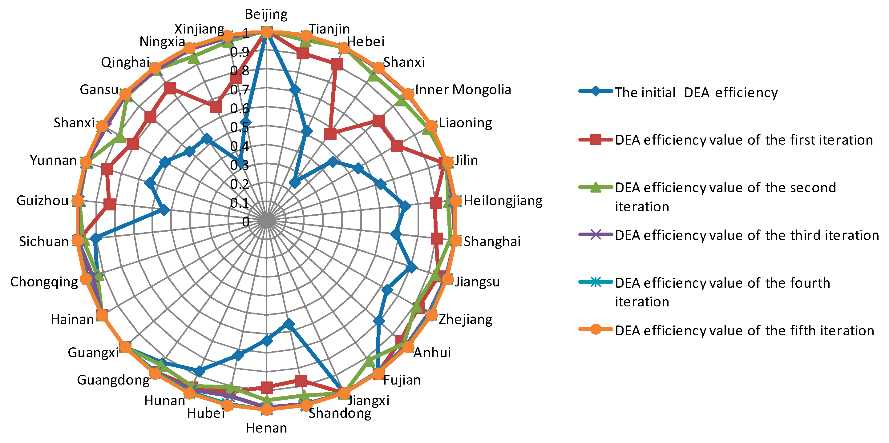
In the next step, the adjusted carbon emission and the consumption of NFFs are used as input variables to calculate the efficiency values of the original DEA model. The average efficiency value of the original DEA model is shown to increase to 0.894, and the efficiency for all provinces and cities has improved significantly from their original state. Compared with the original CO₂ emissions, the CO₂ emissions in Hebei, Shanxi, Inner Mongolia, Liaoning, Jilin, Heilongjiang, Shandong, Henan, Guizhou, Gansu, Qinghai, Ningxia and Xinjiang have all been reduced, in a total amount of 631,691,800 tons of carbon (t.c.). Meanwhile, another 11 provinces and cities, including Beijing, Tianjin, Shanghai, Jiangsu, Zhejiang and Anhui, have accordingly increased their CO₂ emissions by an overall volume of 631,691,800 t.c. The sum of the increased and reduced amounts is zero, guaranteeing the precondition of the fixed total amount. As for another input factor—energy consumption of NFFs—10 provinces and cities, including Tianjin, Hebei, Shanxi and Inner Mongolia, have also reduced their input amount by 158,109,600 t.c.; meanwhile, another 12 provinces and cities, such as Beijing, Liaoning, Jilin and Heilongjiang, have increased their input amount by 158,109,600 t.c., thereby assuring the precondition of fixed total energy consumption. Although the efficiency values of all the provinces and cities have increased following the first iteration, they remain under fair carbon emission allowances. Therefore, another iterative calculation is necessary. After the second iterative adjustment, the average value of the initial DEA efficiency has reached 0.962, with most provinces and cities close to 1. In comparison with the first adjustment, 10 provinces and cities, such as Hebei, Shanxi, Inner Mongolia and Liaoning, continue to reduce their CO₂ emissions, whereas another 12 provinces and cities, including Beijing, Tianjin, Shanghai, and Jiangsu, continue to increase their emissions. In terms of NFF consumption, 10 provinces and cities, such as Tianjin, Shanxi and Inner Mongolia, further reduce their consumption, whereas 14 provinces and cities, such as Beijing, Hebei and Liaoning, must increase their consumption accordingly.

Further adjustments are necessary as a fair and effective carbon emission allocation has not been achieved. After the third iteration, the initial DEA efficiency value reaches 0.991, and almost all the allocative efficiency values nearly reach 0.99. However, further adjustments are undertaken to achieve the most effective efficiency value as expected. The fourth iteration shows that the vast majority of provinces and cities have achieved fair and effective initial efficiency values (reached at 1), apart from a few provinces such as Jiangsu, Fujian, Hubei, Hunan, Guangdong etc. Therefore, a fifth iteration was carried out, as shown in

Table 2. Predicted efficiency values in 2020 using 2010 as a benchmark and taking five iterations.

Region	Initial DEA Efficiency	DEA Efficiency Value of the First Iteration	DEA Efficiency Value of the Second Iteration	DEA Efficiency Value of the Third Iteration	DEA Efficiency Value of the Fourth Iteration	DEA Efficiency Value of the Fifth Iteration
Beijing	1	1	1	1	1	1
Tianjin	0.709	0.906	0.975	0.998	1	1
Hebei	0.519	0.906	1	1	1	1
Shanxi	0.25	0.567	0.95	0.993	1	1
Inner Mongolia	0.467	0.791	0.952	0.997	1	1
Liaoning	0.554	0.788	0.976	0.999	1	1
Jilin	0.628	0.982	1	1	1	1
Heilongjiang	0.73	0.893	0.963	0.987	1	1
Shanghai	0.683	0.898	0.975	0.998	1	1
Jiangsu	0.8	0.952	0.93	0.991	0.996	1
Zhejiang	0.732	0.923	0.908	0.984	0.996	1
Anhui	0.793	0.951	0.97	0.992	1	1
Fujian	1	1	0.915	0.994	0.992	1
Jiangxi	1	1	1	1	1	1
Shandong	0.559	0.867	0.946	0.994	1	1
Henan	0.635	0.883	0.95	0.992	1	1
Hubei	0.728	0.927	0.904	0.951	0.991	1
Hunan	0.872	0.966	0.96	0.981	0.997	1
Guangdong	0.933	0.989	0.948	1	0.992	1
Guangxi	1	1	1	1	1	1
Hainan	1	1	1	1	1	1
Chongqing	0.936	0.987	0.931	0.962	0.991	1
Sichuan	0.904	0.989	0.966	0.993	1	1
Guizhou	0.544	0.831	0.986	0.993	1	1
Yunnan	0.646	0.882	0.992	0.996	1	1
Shanxi	0.618	0.814	0.89	0.975	0.998	1
Gansu	0.547	0.823	0.984	0.992	1	1
Qinghai	0.537	0.867	0.987	0.983	1	1
Ningxia	0.336	0.658	0.945	0.991	1	1
Xinjiang	0.533	0.773	0.97	0.984	1	1

, Table A5 and Figure 1.

After the fifth iteration, the DEA efficiency values of all 30 provinces and cities have become 1. Comparing the initial allocation with the allocation after the fifth iteration, provinces such as Hebei, Shanxi, Inner Mongolia, Liaoning, Jilin, Heilongjiang, Shandong, Henan, Guizhou, Shaanxi, Gansu, Qinghai, Ningxia and Xinjiang all must reduce their carbon emissions, whereas the remaining provinces must increase their carbon emissions; Guangxi, Hainan, etc. demonstrate the most significant increases. Guangxi’s carbon emission increases from 81,762,900 t.c. to 160,709,800 t.c., as shown in Table 1,

Table 3. Predicted CO₂ emission allowance values in 2020 using 2010 as a benchmark.

Region	CO2 *, 0	CO2 *, 1	CO2 *, 2	CO2 *, 3	CO2 *, 4	CO2 *, 5
Beijing	9139.91	12,532.24	13,979.17	14,494.35	14,804.3	14,921.51
Tianjin	9121.63	9854.37	10,049.35	10,327.37	10,546.46	10,629.96
Hebei	44,090.88	30,763.29	25,989.19	26,463.97	27,035.1	27,248.99
Shanxi	39,113.35	21,009.38	14045.3	13,957.53	14,168.89	14,281.07
Inner Mongolia	26,620.04	21,712.03	19,495.64	19,856.89	20,280.97	20,441.53
Liaoning	36,992.38	27,870.89	24,305.74	24,769.18	25,302.13	25,502.38
Jilin	13,487.87	10,915.47	9558.3	9844.67	9920.65	10,000.1
Heilongjiang	18,324.52	15,077.71	13,442.03	13,625.17	13,732.4	13,843.62
Shanghai	16,012.34	16,807.32	16,983.06	17,458.65	17,831.06	17,972.23
Jiangsu	35,754.88	42,785.85	45,971.28	46,879.16	45,195.59	45,101.71
Zhejiang	23,966.21	27,337.58	28,674.44	28,819.88	27,877.03	27,138.91
Anhui	15,409.76	18,907.47	20,322.63	20,603.08	20,885.81	21,055.4
Fujian	10,800.3	16,007.48	18,281.37	16,481.85	16,754.24	16,743.07
Jiangxi	8897.53	12,199.89	13,608.45	14,109.97	14,411.7	14,525.79
Shandong	55,889.96	50,029.84	48,896.29	49,261.04	50,107.18	48,333.68
Henan	33,116.81	32,678.81	32,513.92	32,460.95	32,525.46	32,782.57
Hubei	18,272.22	21,436.2	22,680.89	21,039.75	20,166.37	20,136.15
Hunan	16,870.52	21,128.66	22,880.2	24,120.19	21,824.64	21,919.79
Guangdong	31,925.15	43,772.33	48,825.56	44,301.63	45,404.14	45,344.96
Guangxi	8176.29	12,902.9	15001.14	15610.38	15,944.75	16,070.98
Hainan	2322.3	3184.24	3551.88	3682.78	3761.54	3791.32
Chongqing	7601.55	10,128.85	11192.65	10785.09	10,079.15	10,068.19
Sichuan	17,616.22	24,003.86	26723.52	27118.66	27,241.4	27,454.56
Guizhou	13,197.12	12,769.24	12394.14	12797.92	12,985.58	13,089.43
Yunnan	13,031.79	14,244.31	14625.61	15140.85	15,399.52	15,522.51
Shanxi	15,249.49	16,103.73	14914.46	14314.12	13,896.83	13,979.34
Gansu	9459.62	9041.52	8694.33	8973.79	9094.69	9167.05
Qinghai	2178.34	1974.81	1974.75	2065.16	2078.78	2094.95
Ningxia	5856.23	4101.65	3162.34	3126.23	3188.3	3213.47
Xinjiang	12,639.81	9853.11	8397.38	8644.7	8690.36	8759.82

* CO₂ emission in units of 10 thousand t.c. (tons of carbon, the standard unit of carbon dioxide emissions); 0: The predicted CO₂ emission allowance in 2020 using 2010 as a benchmark and taking no iterations; 1: The predicted CO₂ emission allowance in 2020 using 2010 as a benchmarkand taking the 1st iteration; 2: The predicted CO₂ emission allowance in 2020 using 2010 as a benchmarkand taking the 2nd iteration; 3: The predicted CO₂ emission allowance in 2020 using 2010 as a benchmarkand taking the 3rd iteration; 4: The predicted CO₂ emission allowance in 2020 using 2010 as a benchmarkand taking the 4th iteration; 5: The predicted CO₂ emission allowance in 2020 using 2010 as a benchmarkand taking the 5th iteration.

and Table A5.

For non-fossil energy consumption, Tianjin, Hebei, Shanxi, Inner Mongolia, Shanghai, Jiangsu, Zhejiang, Fujian, Shandong, Hubei, Guizhou, Gansu, Qinghai and Ningxia must reduce their consumption, and the rest of the provinces must increase their consumption; Beijing must increase most. The consumption assigned after five iterations is 1.18 times that of the initial allocation.

Next, we compare our results with past work. Miao et al. [23] researched CO₂ emissions allowances among provinces in 2010 in China but did not research CO₂ emissions allowances among provinces in 2020 in China. References [24,25,26,27,28,29,30,31,32,33,34,35,36] did not use the ZSG-DEA model and/or did not research the CO₂ emissions allowance among provinces in China.

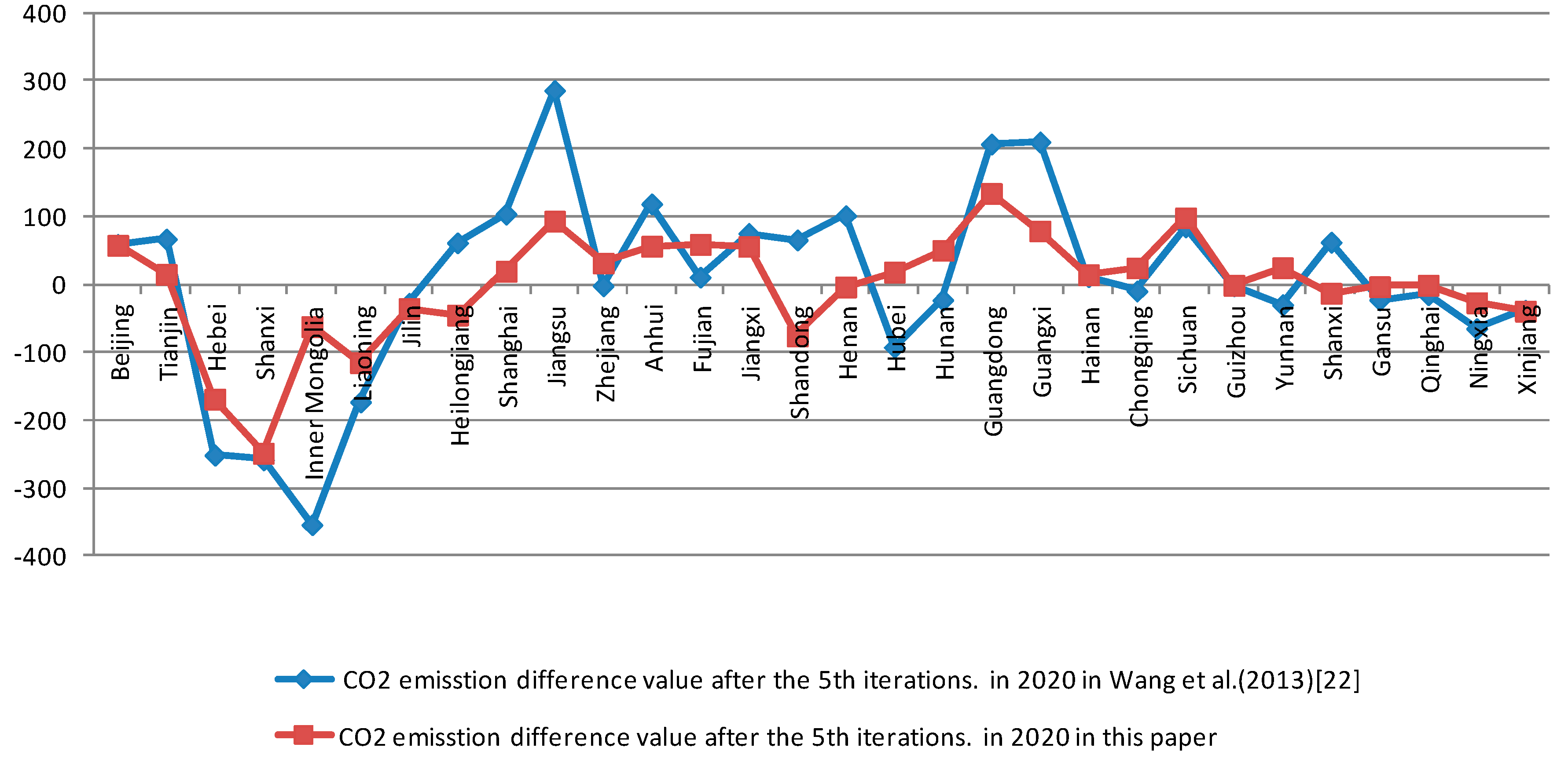
Wang et al. [22] researched CO₂ emission allowances among provinces in 2020 in China using the ZSG-DEA model. Thus, our results are most comparable with Wang et al. [22], and the CO₂ emissions difference values after the 5th iteration in 2020 from both papers are illustrated in Figure 2. Although not all the input and output variables used in Wang et al. [22] are the same as those used in this paper, both papers reveal similar trends in CO₂ emissions difference values for 2020 after the 5th iteration. However, in this paper, the CO₂ emissions difference value in most provinces and cities after the 5th iteration in 2020 is smaller than that in Wang et al. [22]. We investigate the reasons for this difference.

We believe that the main reason for this difference is that the input and output variables in Wang et al. [22] and this paper are not all the same. The input variables used in Wang et al. [22] are total energy consumption, CO₂ emissions and non-fossil energy consumption. All three inputs in Wang et al. [22] have constant total amounts that must be reallocated among China’s regions. The output variables used in Wang et al. [22] are GDP (based on 2005 prices) and POP. Our article uses CO₂ emissions and non-fossil energy consumption as input variables; we do not use total energy consumption because we posit that this variable is changeable. The output variables used in our article are total energy consumption, gross domestic product (based on 2010 prices) and POP.

4. Methodology

4.1. BBC-DEA Model

It is presumed that each assessment system has a number (n) of the same types of DMUs and that each unit has a number (r) input indexes and a number (m) of output indexes. The equation for the BBC-DEA model of the relative efficiency assessment of DMU₀ is set forth as Equation (1), in which θ₀ represents the relative efficiency of DMU₀, while λ_i indicates the ratio of each DMU_i in a restructured and effectively combined decision unit relative to DMU₀:

$$\begin{array}{c}\min {\mathsf{\theta }}_{\mathrm{o}}\\ s.t.{\displaystyle \sum _{i=1}^n{\mathsf{\lambda }}_i{y}_{ij}}\ge y_{oj},j=1,2,3,\mathrm{...},m\\ {\displaystyle \sum _{i=1}^n{\mathsf{\lambda }}_i{x}_{ik}\le {\mathsf{\theta }}_{\mathrm{o}}}{x}_{\mathrm{o}k},k=1,2,3,\mathrm{...}r\\ {\displaystyle \sum _{i=1}^n{\mathsf{\lambda }}_i=1,i=1,2,3,\mathrm{...}n}\\ {\mathsf{\lambda }}_i\ge 0,i=1,2,3,\mathrm{...}n\end{array}$$

(1)

The input and output variables of the classic DEA model (CCR, BBC, etc.) are relatively independent. Given any of the DMUs, its input or output will not affect any other DMU’s input or output variables. A classic DEA model only demonstrates the relative efficiency of the original state. However, under the condition of competition, the amount of input or output for variables should be restricted for the constant total, and the input and output of each DMU are related to one another to ensure this constant. If one of the inefficient DMUs increases its input or output to achieve a greater efficiency frontier, other DMUs must reduce their input or output, which strays from the assumptions of the classic DEA model. This characteristic conforms exactly to the feature of a ZSG, which requires that the loss or earnings of a stakeholder be the earnings or loss of other stakeholders to ensure that the total earning amount is zero.

4.2. Zero Sum Earning DEA Model

The initial ZSG-DEA model was proposed by Gomes and Lins [37] on the basis of an input-oriented CCR-DEA model. To realize an effective DEA model, DMU₀ must reduce the amount of input k as u₀ = x_0k(1 − φ₀) and allocate this amount proportionally to other DMUs. Thus, the input allocation value acquired by the i^th DMU is x_ik/Σx_ik·x_0k(1 − φ₀). As all the DMUs experience a certain increase or decrease of input proportion simultaneously, the reallocation of input k after adjustment is:

$$x_{ik}^{\prime }={\displaystyle \sum }_{o\ne i}\left[\frac{x_{ik}}{{{\displaystyle \sum }}_{i\ne o}{x}_{ik}}\cdot x_{ok}\left(1-{\mathsf{\phi }}_o\right)\right]-x_{ik}\left(1-{\mathsf{\phi }}_i\right),i=1,2,3,\mathrm{...}n$$

(2)

In this study, it is assumed that more inputs have fixed total amounts. When a DMU aims for increased efficiency, different proportions of increase or decrease of a fixed total amount follow. Meanwhile, it is believed that fixed earnings are effective at setting a scope, such that when a DMU operates within an optimum scope, the application of the variable’s earnings become more reasonable. In addition, because each DMU in this study, whether big or small or in different developing phases, can be distinguished from one other, our assumption is that not all the DMUs operate within the optimum scope:

$$\begin{array}{c}{E}_{\text{ZSG}}=\min {\displaystyle \sum _{i=1}^m{w}_i{\mathsf{\theta }}_i}\\ s.t.{\displaystyle \sum _{j=1}^n{\mathsf{\lambda }}_j{y}_{rj}\ge y_{rk}},r=\mathrm{1....}s\\ {\displaystyle \sum _{j=1}^n{\mathsf{\lambda }}_j{x}_{ij}(1+\frac{x_{ik}(1-{\mathsf{\theta }}_i)}{{\displaystyle \sum _{j=1,j\ne k}^n{x}_{ij}}}})\le {\mathsf{\theta }}_i{x}_{ik},i=\mathrm{1....}m\\ {\displaystyle \sum _{i=1}^m{w}_i=1},w_i\ge 0,i=\mathrm{1....}m\\ {\mathsf{\lambda }}_j\ge 0,j=\mathrm{1....}n\end{array}$$

(3)

where θ_i is the measurement of the efficiency of ZSG-DEA related to the number (i) of DMUs in Equation (3), when all i inputs are limited under fixed conditions; w_i is the weight of θ_i; E_ZSG is the efficiency of the average value of the uniform weight of each DMU; x_ij and y_rj are the input and output values, respectively; x_ik and y_rk refer to the input and output values, respectively, of the DMU in their assessment; and λ_i is the contribution rate of effective planning made by each DMU.

4.3. A Zero Sum Gains Data Envelopment Analysis Model for CO₂ Allowance Allocation in China

To reflect the demographic and economic characteristics of each region in the process of allowance allocation, the output variables used in the optimized ZSG-DEA model are GDP, POP and energy consumption in 2010. The input variables are CO₂ emission and consumption of non-fossil fuels (NFFs). These two inputs have a fixed total amount and must be reallocated among provinces. The ZSG-DEA model for China is as follows:

$$\begin{array}{c}{E}_{\text{ZSG}}^{\prime }=\min w^{\text{co2}}{\mathsf{\theta }}^{\text{co2}}+w^{\text{NF}}{\mathsf{\theta }}^{\text{NF}}\\ s.t.{\displaystyle \sum _{j=1}^n{\mathsf{\lambda }}_j{y}_j^{\text{GDP}}}\ge y_k^{\text{GDP}}\\ {\displaystyle \sum _{j=1}^n{\mathsf{\lambda }}_j{y}_j^{\text{POP}}}\ge y_k^{\text{POP}}\\ {\displaystyle \sum _{j=1}^n{\mathsf{\lambda }}_i}{y}_j^{\text{TE}}\ge y_j^{\text{TE}}\\ {\displaystyle \sum _{j=1}^n{\mathsf{\lambda }}_j{x}_j^{\text{co2}}(1+\frac{x_k^{\text{co2}}(1-{\mathsf{\theta }}^{\text{co2}})}{{\displaystyle \sum _{j=1,j\ne k}^n{x}_j^{\text{co}2}}}}\le {\mathsf{\theta }}^{\text{co2}}{x}_k^{\text{co2}}\\ {\displaystyle \sum _{j=1}^n{\mathsf{\lambda }}_j{x}_j^{\text{NF}}(1+\frac{x_k^{\text{NF}}(1-{\mathsf{\theta }}^{\text{NF}})}{{\displaystyle \sum _{j=1,j\ne k}^n{x}_j^{\text{NF}}}}})\le {\mathsf{\theta }}^{\text{NF}}{x}_k^{\text{NF}}\\ w^{\text{co2}}+w^{\text{NF}}=1,w^{\text{co2}}>0;w^{\text{NF}}>0\\ {\mathsf{\lambda }}_i\ge 0,j=\mathrm{1....}n\end{array}$$

(4)

where θ^CO2 and θ^NFF represent the efficiency of the CO₂ emission allocation and that of NFF consumption, respectively. Likewise, w^CO2 and w^NFF are the weights of the two aforementioned efficiencies, respectively. We set the weight to 1/2, as both efficiencies are regarded as equally important. Equation (4) is the specific application of Equation (3) to the allocative efficiency of carbon emission reduction at the provincial level in 2020 in China.

Equation (4) indicates that when various regions have the same level of carbon emission and NFF energy consumption, the region with the smaller POP and GDP has relatively low efficiency; when different regions have the same level of carbon emission and NFF energy consumption, the region with the larger POP and GDP has greater efficiency.

The transmission mechanism is described as follows. At first, all regions are not at the new ZSG-DEA frontier in China due to erroneous CO₂ emission allocations among different regions in China. Then, all the regions draw close to the new ZSG-DEA frontier because of a change in the amounts of CO₂ emissions in different regions in China. Finally, all regions are at the new ZSG-DEA frontier in China due to a change in the amounts of CO₂ emissions allocated to the different regions in China. The transmission mechanism is also depicted in Figure 3, where MN indicates the DEA frontier and EF indicates the ZSG-DEA frontier that is required to achieve an efficiency value of 1 by the fifth iteration.

Region A and region B are not on the EF. By changing the amounts of CO₂ emissions allocated to different regions, they move onto the EF. The input variables used are carbon dioxide emissions and NFF consumption. The output variables used in the optimized ZSG-DEA model are GDP, POP and energy consumption, as shown in Figure 3.

5. Data Sources and Processing

This paper examines the carbon emission allowance allocation mode of all Chinese provinces in terms of efficiency. Therefore, the allocation allowance of all provinces must be first affirmed, and then the efficiency of the allocation mode may be examined. This study assumes that overall carbon emission in 2015 is 17% less than that in 2010, which is consistent with the goal of carbon emission reduction in the “12th Five Year Plan”. At the Copenhagen United Nations Climate Change Conference, the Chinese government pledged that its carbon emission in 2020 would be reduced by 40%–45% from that its 2005 levels.

These results show that China’s carbon emission reduction goal for 2020 will be approximately 31.3% if the 2010 value is taken as the benchmark. After affirming the total amount of the allocation, the carbon emissions allowance for each province can be simulated in terms of the optimum allocation of efficiency.

Using 2010 as the base year, the total amount of carbon emissions in 2020 and its allocation to each province and city can be estimated and predicted with optimal efficiency. The table below presents the carbon emissions, energy consumption, GDP, POP, etc., in all provinces and cities in 2010, which are used as the initial data (see

Table 4. Data from 2010.

Region	GDP *	POP **	TEC ***	CDE ****	NFEC *****	The Initial DEA Efficiency Value
Beijing	13,723	1755	9038.53	1535.05	323.23	1.000
Tianjin	9720	1228	10,263.82	7592.48	683.32	0.537
Hebei	20,255	7034	49,853.14	12,222.90	2455.54	0.726
Shanxi	8529	3427	53,262.19	74321.14	2590.73	0.735
Inner Mongolia	11,981	2422	7908.22	83,730.53	2963.12	0.148
Liaoning	18,263	4319	39,905.99	13,182.51	1519.04	0.939
Jilin	8684	2740	13,802.69	6438.69	768.13	0.656
Heilongjiang	9950	3826	22,457.83	16,860.45	904.54	0.888
Shanghai	17,959	1921	16,687.51	2696.97	1157.72	0.849
Jiangsu	40,516	7725	39,186.97	6253.51	4061.85	0.730
Zhejiang	27,154	5180	24,316.20	3908.13	2834.07	0.701
Anhui	12,120	6131	18,184.14	13,618.62	1752.55	0.625
Fujian	14,369	3627	12,201.62	4670.97	1656.69	0.393
Shanxi	9433	4432	10,315.92	1166.16	784.10	1.000
Shandong	39,787	9470	63,189.12	24,583.15	3765.66	0.600
Henan	22,619	9487	41,340.85	23,572.29	2701.34	0.640
Hubei	15,638	5720	20,135.70	1246.26	2478.89	1.000
Hunan	15,245	6406	15,979.85	7907.36	1356.82	0.837
Guangdong	45,963	9638	33,264.81	9290.76	3436.28	0.559
Guangxi	8910	4856	10,620.27	2321.48	1269.56	0.677
Hanan	2105	859	2857.06	1364.91	169.60	0.909
Chongqing	8562	2859	8595.60	5065.61	605.90	0.843
Sichuan	16,745	8185	21,082.59	11,349.42	2095.45	0.694
Guzhou	4421	3798	13,270.06	15,446.41	1618.59	0.422
Yunan	7336	4571	13,435.03	9687.58	1670.21	0.488
Shaanxi	10,285	3772	16,946.43	42,016.28	1177.38	0.585
Gansu	3810	2635	9488.83	5217.85	1049.57	0.452
Qinghai	1250	557	2751.52	2850.40	580.09	0.176
Ningxia	1610	625	8673.02	7039.19	695.61	0.446
Xinjiang	4983	2159	15,049.29	17,993.44	768.13	0.701
Total	431,925	131,364	624,064.79	435,150.50	49,893.71

* Unit: 100 million Chinese Yuan; ** Population (unit: 10 thousand Chinese Yuan); *** Total energy consumption (unit: 10 thousand tce, where tce is tons of standard coal, the unified standard unit of heat value); **** CO₂ emissions (Unit: 10 thousand t.c., where t.c. is tons of carbon, the standard unit of CO₂ emissions); ***** Non-fossil energy consumption (Unit: 10 thousand tce).

).

The calculation of actual carbon emission in each province and city is derived from the amount of energy consumption in the energy balance sheets for all provinces and cities in the China Energy Statistical Yearbook 2011 [38,39,40,41,42,43,44]. The detailed calculation methods for carbon emission are described in the Guidelines for the Provincial Greenhouse Gas List [45], which is also called IPCC Method 1. According to this method, actual carbon emission is derived from the consumption of various fossil fuels, the heat per unit and carbon content per unit of various types of fuels plus the average oxidation rate of the main equipment used to burn various fuels, after deducting fixed carbon content and other parameters of fossil fuels used for non-energy purposes. However, it has been proven that it is difficult to acquire certain data in the calculation process, such as the number of products with fixed carbon content, etc. Therefore, an alternative method is employed in this study and is demonstrated below.

First, the energy consumption of different types of fossil fuels is converted into that of standard coal, and then the carbon emission factor, fixed carbon rate, oxidation rate of carbon and other parameters are used to calculate the emission amount of carbon and carbon dioxide in different types of fuels. The specific equation for the calculation is as follows:

X_i = Σproduction + import − export ± increase or decrease of stock ± others (mainly adding fuels overseas)

The emission amount of carbon (PC) is as follows:

$$PC={\displaystyle \sum _{i=1}^n\left[k_i\times ({\mathsf{\lambda }}_i{\mathsf{\phi }}_i-{\mathsf{\theta }}_i)\times X_i\right]}$$

(5)

where k is the carbon oxidation rate; λ is the conversion coefficient of standard coal; φ is the potential carbon emission factors; and θ is the solid carbon rate.

X_i represents the total energy consumption in the i^th province or city. The parameters of other models also can be found in

Table 5. Model parameters.

Fuels	CCSC (λ) *	PCEF (φ) **	SCR (θ) ***	COR (k) ****
Raw coal	0.7143	27.3	0.3	0.98
Washed coal	0.9	25.8	0.3	0.98
Other washed coal	0.5253	25.8	0.3	0.98
Coking coal	0.9714	29.5	0.3	0.98
Crude oil	1.4286	29.5	0.8	0.99
Gasoline	1.4714	18.9	0.8	0.99
Kerosene	1.4714	19.6	0.75	0.99
Diesel	1.4571	20.2	0.8	0.99
Heavy oil	1.4286	21.1	0.5	0.99
Natural gas	1.33	15.3	0.33	0.995
Coke oven gas	6.1417	29.5	0.3	0.995
Other gas	2.8758	29.5	0.3	0.995
Refinery dry gas	1.5714	20	0.5	0.995
Liquefied petroleum gas (LPG)	1.7143	17.2	0.8	0.99
Type coal	0.6068	25.8	0.3	0.98
Other petroleum products	1.3107	20	0.8	0.99
Other coking products	1.154	25.8	0.3	0.98

* The conversion coefficient of standard coal (λ); ** Potential carbon emission factors (φ); *** Solid carbon rate (θ); **** Carbon oxidation rate (k).

[46]. Because the molecular weight of CO₂ is 44 and the molecular weight of carbon is 12, the total carbon emission of each province calculated above can be converted into CO₂ emission, based on this ratio. For the energy conversion, the conversion coefficient used in this study is 29,307.6 MJ of heat of standard coal per ton (see Table 5).

The data regarding NFFs are calculated on the basis of the Annual Development Report of China’s Power Sector 2011 [47], issued by the China Electricity Council. NFFs refer to energy resources that are not coal, petroleum, natural gas or others; thus, NFFs consist of those resources that are not formed through long-term geological transformation that can only be consumed once and instead include current new energies and renewable energies such as nuclear energy, wind energy, solar energy, water energy, etc. According to the actual praxis and the available data, the hydroelectric and thermal energy data of NFFs are calculated for the consumption of non-fossil energy and converted into standard coal, derived from the conversion standard of 0.1229 standard coal/KW that is based on the national standard found in GB-2008 [48].

The data for GDP and the populations of provinces in 2010 are obtained from the China Statistical Yearbook 2011. According to the Energy Information Administration (EIA), the United States energy information administration website and the International Energy Outlook [49], the predicted average annual growth rate of GDP for China is 6.6% from 2010 to 2030, which is used in this study for projecting GDP in 2020. Moreover, China’s population will reach 1.43 billion by 2020 in accordance with World Population Prospects [50], published by the United Nations Department of Economic and Social Affairs (UNDESA). The prediction of total energy consumption in 2020 is calculated using the energy/GDP elasticity coefficient. As for the energy consumption goal of NFFs, based on the medium- and long-term plans of national renewable energy development, non-fossil energies should account for 15% of primary energy consumption by 2020. The consumption ratio of NFFs over primary energy equals the energy consumption of NFFs/the total consumption of primary energy (fossil fuels + consumption of NFFs). This calculation is used to predict the energy consumption of NFFs in 2020.

The total amount of national carbon dioxide emission in 2020 is predicted to be 5,711,350,300 t.c. Taking the carbon emission of all provinces and cities from 2010–2014 and the overall allowance into consideration, the predicted values of initial allowance allocation results and other variables are shown in Table 1.

6. Conclusions

From the perspective of allocative efficiency, carbon emission allowances for China’s 30 provinces and cities are allocated in this study by employing a ZSG-DEA model. The carbon dioxide emissions index and non-fossil energy consumption index for 2020 are calculated by taking the emission reduction target in the “12th Five Year Plan” as the baseline. Then, the optimal allocation scheme for all provinces and cities in 2020 is achieved under fixed total volumes of carbon emissions and non-fossil energy consumption. As the largest country in the world in terms of overall carbon emission, China must reduce its carbon emissions to improve environmental quality. Therefore, it is important for China to set up carbon emission targets among provinces and cities during the next five years (the “13th Five Year Plan”, which covers from 2016 to 2020), which would be more efficient and fair. We therefore suggest that provinces such as Hebei, Shanxi, Inner Mongolia, Liaoning, Jilin, Heilongjiang, Shandong, Henan, Guizhou, Shaanxi, Gansu, Qinghai, Ningxia and Xinjiang must reduce their carbon emissions. The rest of the provinces remain unchanged or reduce their carbon emissions although the rest of the provinces will increase their carbon emissions when applying zero sum gains analysis, with Guangxi and Hainan having the most significant increases, as reflected in Table 3. For non-fossil energy consumption, Tianjin, Hebei, Shanxi, Inner Mongolia, Shanghai, Jiangsu, Zhejiang, Fujian, Shandong, Hubei, Guizhou, Gansu, Qinghai and Ningxia must reduce consumption, and the remaining provinces must increase consumption, with Beijing needing to increase consumption the most.

References

1. Ding, D.; Feng, J. The choices of the carbon allowances allocation methods in our country. Int. Bus. 2013, 4, 83–92. [Google Scholar]
2. Sun, D.; Ma, X. The research of the methods of initial allocation of carbon allowances. Ecol. Econ. 2013, 2, 81–85. [Google Scholar]
3. Yin, Y.; Cui, M. The research of “China plan” in the international carbon financial system construction. Int. Financ. Res. 2010, 12, 59–66. [Google Scholar]
4. Wang, Y. The Way of Carbon Emissions Trading System of China: International Practice and Application in China; Economics and Management Press: Beijing, China, 2011. [Google Scholar]
5. Jiang, J. On carbon quota distribution on a limited rationality repeat gam e. China Open. J. 2013, 3, 18–35. (In Chinese) [Google Scholar]
6. Cong, R. The design of carbon allowance auction mechanism: Based on the research on multi-agents model. Rev. Econ. Prod. 2013, 1, 113–124. [Google Scholar]
7. Wang, K.; Li, M. The DEA model and application of carbon emission allocation. J. Beijing Inst. Technol. 2013, 4, 7–13. [Google Scholar]
8. Rogge, K.S.; Hoffmann, V.H. The impact of the EU ETS on the sectoral innovation system for power generation technologies—Findings for germany. Energy Policy 2010, 38, 7639–7652. [Google Scholar] [CrossRef]
9. Sandoff, A.; Schaad, G. Does EU ETS lead to emission reductions through trade? The case of the Swedish emissions trading sector participants. Energy Policy 2009, 37, 3967–3977. [Google Scholar] [CrossRef]
10. Zhang, Y.-J.; Wei, Y.-M. An overview of current research on EU ETS: Evidence from its operating mechanism and economic effect. Appl. Energy 2010, 87, 1804–1814. [Google Scholar] [CrossRef]
11. Oestreich, A.M.; Tsiakas, I. Carbon emissions and stock returns: Evidence from the EU emissions trading scheme. J. Bank. Financ. 2015, 58, 294–308. [Google Scholar] [CrossRef]
12. Jong, T.; Couwenberg, O.; Woerdman, E. Does EU emissions trading bite? An event study. Energy Policy 2014, 69, 510–519. [Google Scholar] [CrossRef]
13. Bushnell, J.B.; Chong, H.; Mansur, E.T. Profiting from regulation: Evidence from the European carbon market. Am. Econ. J. Econ. Policy 2013, 5, 78–106. [Google Scholar] [CrossRef]
14. Zeng, S.; Hu, M.; Su, B. Research on investment efficiency and policy recommendations for the culture industry of China based on a three-stage DEA. Sustainability 2016, 8, 324. [Google Scholar] [CrossRef]
15. Zofı́o, J.L.; Prieto, A.M. Environmental efficiency and regulatory standards: The case of CO2 emissions from OECD industries. Resour. Energy Econ. 2001, 23, 63–83. [Google Scholar] [CrossRef]
16. Lozano, S.; Gutiérrez, E. Non-parametric frontier approach to modelling the relationships among population, GDP, energy consumption and CO2 emissions. Ecol. Econ. 2008, 66, 687–699. [Google Scholar] [CrossRef]
17. Lins, M.P.E.; Gomes, E.G.; De Mello, J.C.C.B.S.; De Mello, A.J.R.S. Olympic ranking based on a zero sum gains DEA model. Eur. J. Oper. Res. 2003, 148, 312–322. [Google Scholar] [CrossRef] [Green Version]
18. Lin, T.; Ning, J. The research on the carbon emission permit allocative efficiency in EU countries based on zero and DEA model. J. Quant. Tech. Econ. 2011, 3, 36–50. [Google Scholar]
19. Sun, Z.; Zhou, D.; Zhou, P.; Miao, Z. The allocation of the energy-saving index based on the environment ZSG-DEA. Syst. Eng. 2012, 1, 84–90. [Google Scholar]
20. Wu, X.; Tan, L.; Guo, J.; Wang, Y.; Liu, H.; Zhu, W. A study of allocative efficiency of PM2.5 emission rights based on a zero sum gains data envelopment model. J. Clean. Prod. 2016, 113, 1024–1031. [Google Scholar] [CrossRef]
21. Pang, R.-Z.; Deng, Z.-Q.; Chiu, Y.-H. Pareto improvement through a reallocation of carbon emission quotas. Renew. Sustain. Energy Rev. 2015, 50, 419–430. [Google Scholar] [CrossRef]
22. Wang, K.; Zhang, X.; Wei, Y.-M.; Yu, S. Regional allocation of CO2 emissions allowance over provinces in China by 2020. Energy Policy 2013, 54, 214–229. [Google Scholar] [CrossRef]
23. Miao, Z.; Geng, Y.; Sheng, J. Efficient allocation of CO2 emissions in China: A zero sum gains data envelopment model. J. Clean. Prod. 2016, 112, 4144–4150. [Google Scholar] [CrossRef]
24. Tietenberg, T. The tradable-permits approach to protecting the commons: Lessons for climate change. Oxf. Rev. Econ. Policy 2003, 19, 400–419. [Google Scholar] [CrossRef]
25. Fischer, C. Combining rate-based and cap-and-trade emissions policies. Clim. Policy 2003, 3, S89–S103. [Google Scholar] [CrossRef]
26. Quirion, P. Historic versus output-based allocation of GHG tradable allowances: A comparison. Clim. Policy 2009, 9, 575–592. [Google Scholar] [CrossRef]
27. Fischer, C.; Fox, A.K. Output-based allocation of emissions permits for mitigating tax and trade interactions. Land Econ. 2007, 83, 575–599. [Google Scholar] [CrossRef]
28. Yuan, Y.-N.; Shi, M.-J.; Li, N.; Zhou, S.-L. Intensity allocation criteria of carbon emissions permits and regional economic development in China—Based on a 30-province/autonomous region computable general equilibrium model. Adv. Clim. Chang. Res. 2012, 3, 154–162. [Google Scholar]
29. Xu, J.; Yang, X.; Tao, Z. A tripartite equilibrium for carbon emission allowance allocation in the power-supply industry. Energy Policy 2015, 82, 62–80. [Google Scholar] [CrossRef]
30. Paloheimo, E.; Salmi, O. Evaluating the carbon emissions of the low carbon city: A novel approach for consumer based allocation. Cities 2013, 30, 233–239. [Google Scholar] [CrossRef]
31. Zhang, Y.-J.; Wang, A.-D.; Da, Y.-B. Regional allocation of carbon emission quotas in China: Evidence from the shapley value method. Energy Policy 2014, 74, 454–464. [Google Scholar] [CrossRef]
32. Yu, S.; Wei, Y.-M.; Wang, K. Provincial allocation of carbon emission reduction targets in China: An approach based on improved fuzzy cluster and shapley value decomposition. Energy Policy 2014, 66, 630–644. [Google Scholar] [CrossRef]
33. Pan, X.; Teng, F.; Ha, Y.; Wang, G. Equitable access to sustainable development: Based on the comparative study of carbon emission rights allocation schemes. Appl. Energy 2014, 130, 632–640. [Google Scholar] [CrossRef]
34. Gao, G.; Chen, S.; Yang, J. Carbon emission allocation standards in China: A case study of Shanghai city. Energy Strategy Rev. 2015, 7, 55–62. [Google Scholar] [CrossRef]
35. Feng, C.; Chu, F.; Ding, J.; Bi, G.; Liang, L. Carbon emissions abatement (CEA) allocation and compensation schemes based on DEA. Omega 2015, 53, 78–89. [Google Scholar] [CrossRef]
36. Ren, J.; Bian, Y.; Xu, X.; He, P. Allocation of product-related carbon emission abatement target in a make-to-order supply Chain. Comput. Ind. Eng. 2015, 80, 181–194. [Google Scholar] [CrossRef]
37. Gomes, E.G.; Lins, M.P.E. Modelling undesirable outputs with zero sum gains data envelopment analysis models. J. Oper. Res. Soc. 2008, 59, 616–623. [Google Scholar] [CrossRef]
38. The National Bureau of Statistics. China Energy Statistical Yearbook; China Statistics Press: Beijing, China, 2011.
39. The National Bureau of Statistics. China Energy Statistical Yearbook 2013; China Statistics Press: Beijing, China, 2013.
40. The National Bureau of Statistics. China Statistical Yearbook 2011; China Statistics Press: Beijing, China, 2011.
41. The National Bureau of Statistics. China Statistical Yearbook 2012; China Statistics Press: Beijing, China, 2012.
42. The National Bureau of Statistics. China Statistical Yearbook 2013; China Statistics Press: Beijing, China, 2013.
43. The National Bureau of Statistics. China Statistical Yearbook 2014; China Statistics Press: Beijing, China, 2014.
44. The National Bureau of Statistics. China Statistical Yearbook 2015; China Statistics Press: Beijing, China, 2015.
45. The Department of Dealing with Climate Changes in National Development and Reform Commission. Greenhouse Gases at the Provincial Level Listing Compilation Guidelines. 2011. Available online: http://www.cbcsd.org.cn/sjk/nengyuan/standard/home/20140113/download/shengjiwenshiqiti.pdf (accessed on 28 April 2016).
46. Sun, T.; Zhao, T. The research on measurement of carbon emission and its trend. Audit. Econ. Res. 2014, 2, 104–111. [Google Scholar]
47. Chinese Electricity Business Council. The Annual Report of the Development of Chinese Electricity Industry in 2011; China Market Press: Beijing, China, 2011. [Google Scholar]
48. China’s National Standard Management Committee. The General Principles of the Comprehensive Energy Consumption Calculation(GB/T 2589-2008); China Standard Publishing House: Beijing, China, 2008.
49. Energy Information Administration (EIA). International Energy Outlook 2009; Energy Information Administration: Washington, DC, USA, 2009.
50. World Population Prospects: The 2008 Revision. Un Department of Economic and Social Affairs; United Nations Department of Economic and Social Affairs (UNDESA): New York, NY, USA, 2009.
Figure 1. Predicted efficiency values in 2020 using 2010 as a benchmark and taking five iterations.
Energies 09 00329 g001
Figure 2. The trend of CO2 emission difference values after the 5th iteration in 2020 between this paper and Wang et al. [22].
Energies 09 00329 g002
Figure 3. The transmission mechanism from the DEA frontier to the zero sum gains data envelopment analysis (ZSG-DEA) frontier.
Energies 09 00329 g003