Diagnostic Measurements for Power Transformers

Abstract

With the increasing age of the primary equipment of the electrical grids there exists also an increasing need to know its internal condition. For this purpose, off- and online diagnostic methods and systems for power transformers have been developed in recent years. Online monitoring is used continuously during operation and offers possibilities to record the relevant stresses which can affect the lifetime. The evaluation of these data offers the possibility of detecting oncoming faults early. In comparison to this, offline methods require disconnecting the transformer from the electrical grid and are used during planned inspections or when the transformer is already failure suspicious. This contribution presents the status and current trends of different diagnostic techniques of power transformers. It provides significant tutorial elements, backed up by case studies, results and some analysis. The broadness and improvements of the presented diagnostic techniques show that the power transformer is not anymore a black box that does not allow a view into its internal condition. Reliable and accurate condition assessment is possible leading to more efficient maintenance strategies.

1. Introduction

The reliability of the electrical power system depends on the performance and availability of its components such as power transformers. Due to the increasing age of the transformer population condition assessment and thus onsite diagnostics are important issues to secure a reliable operation of the electrical power system. During the last decades, major works are being carried out for development of reliable and accurate condition assessment techniques [1]. Offline methods require disconnecting the transformer from the power network and are mainly used during scheduled inspections or when the transformer is already failure suspicious. In comparison to this, online methods are used during the operation and offer a possibility to record the condition under realistic operating conditions (e.g., electric field, load, and temperature). Monitoring is the continuous application of online measurement techniques which allows trending and the early detection of an oncoming fault by automatic evaluation of these data. The applicability of the different condition assessment techniques are depicted in

Table 1. Status of different condition assessment techniques. DGA: dissolved gas analysis; PD: partial discharge, IEC: International Electrotechnical Commission, UHF: ultra-high frequency, FRA: frequency response analysis, PDC: polarization and depolarization currents, FDS: frequency domain spectroscopy.

Method	Offline	Online	Monitoring	Offsite
Ageing of oil (e.g., color, moisture, and tan δ)	xxx	xXx	x 1	xxx
Furan in oil analysis	xX	XX	-	XX
Gas-in-oil analysis (DGA)	xxx	xXx	xXx	xxx
PD (IEC 60270)	xxx	XX	X	XXX
Unconventional PD-measurement (e.g., UHF PD measurement)	xx	XX	X	XX
Transfer function (FRA)	xxX	X	-	XXX
Dielectric diagnostic (PDC and FDS)	xx	-	-	XX
Thermal monitoring	-	-	XX	-
Degree of polymerization (DP-value)	-	-	-	XXX

XXX: generally accepted or standardized; XX: accepted by different users; X: under investigation or consideration; ¹ moisture measurement; and -: not applicable.

.

Localized internal insulation failures can lead to catastrophic breakdown. To reduce such risk, power transformers have to pass a range of factory tests including one for partial discharge (PD) activity before acceptance and commissioning. Onsite PD measurements are often restricted by high site interference. Hence the electrical PD-measurement set-up according to International Electrotechnical Commission (IEC) 60270 [2] usually has sensitivity limitations for onsite/online measurements. In contrast, the sensitivity of unconventional ultra-high frequency (UHF) PD measurements is sufficient and normally not affected by external disturbances. Especially in noisy surroundings, it is a helpful method to support other PD diagnostic techniques for example acoustic localization of PD.

Frequency response analysis (FRA) compares measured transfer functions of power transformers. Deviations between frequency response curves indicate electrical or mechanical damages of windings. Interpretation of the deviations between transfer functions is not a standardized process and promises to be more reliable and meaningful if skilled knowledge about the transformer design is incorporated.

Especially, the established dissolved gas analysis (DGA) can provide relevant information about internal transformer faults. Natural aging, thermal and electrical failures generate typical fault gases, which dissolve in the insulating oil. By analyzing these fault gas profiles, evaluation of kind and severity of the fault can be estimated. Online monitoring of the content of dissolved gases is a powerful tool, enabling the control of fault gas development continuously and thus guaranteeing an optimal energy transmission.

Another factor is the assessment of the transformer’s ageing condition. Ageing depends directly on operating temperature and time. The limiting factor of lifetime is the degradation of paper insulation. This goes hand in hand with moisture production from the ageing process. Thus, by knowing the moisture content in the solid insulation, it is possible to get an idea of the ageing condition and decide further actions. Moisture assessment can be done in various ways. For onsite offline measurements, dielectric spectroscopy is a viable tool. Moisture has an effect on the dielectric response of the insulating system. Among different methods frequency domain spectroscopy (FDS) will be presented in detail.

The lifetime performance of a power transformer strongly depends on the temperatures its materials have been exposed to. Because of their significant effect, a profound knowledge about these temperatures is of great interest. Due to transient load conditions, changing ambient conditions, adjustable cooling systems and their design and operation principles, transformers represent a rather complex thermal system. In addition, the particular design of a certain transformer, with its applied materials and installed components, complicates precise simulations tremendously. However, knowledge about the exact temperature distribution inside a transformer may not be necessary within the scope of every desired application. For instance, the determination of a constant, non-critical level of overload might already be achieved by means of a simplified thermal model which additionally can offer the possibility of monitoring of the operational state of the cooling unit.

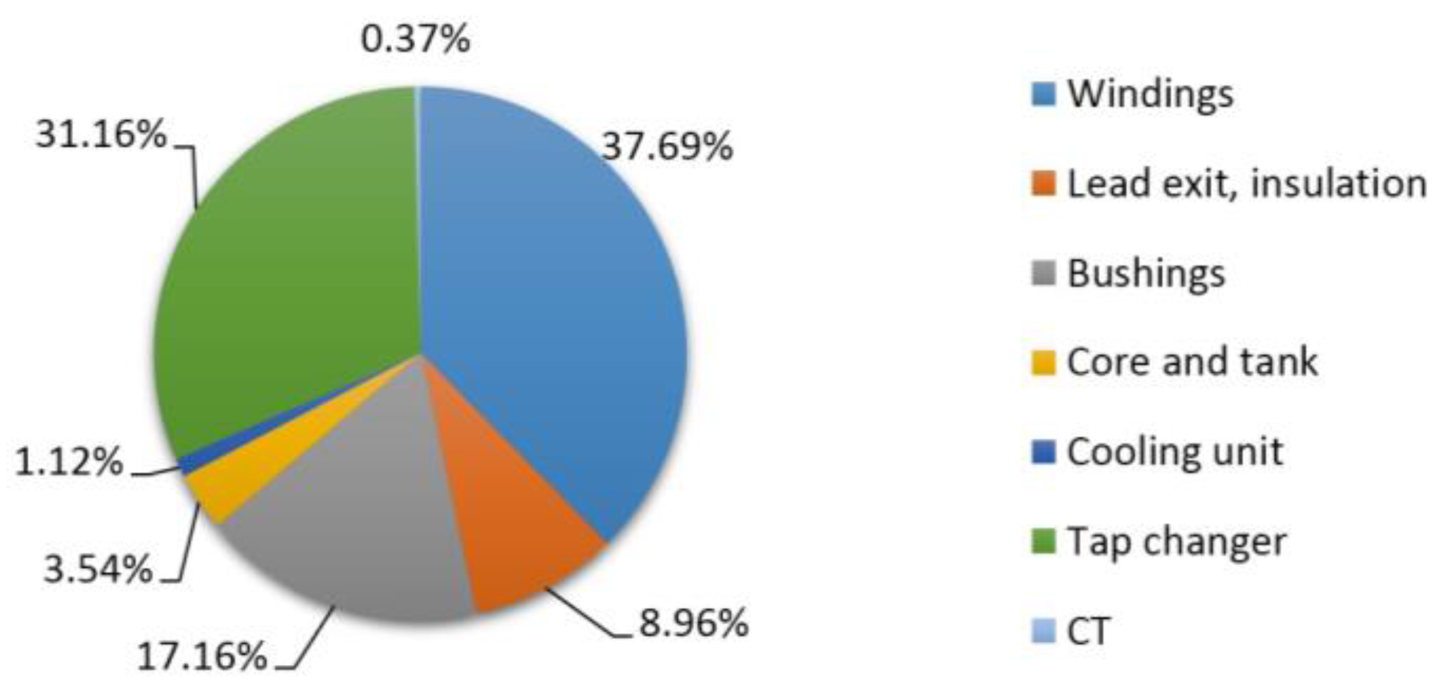
2. Failure Statistic of Power Transformers

Accurate information about service experience of high voltage (HV) equipment is of great importance for both manufacturers and utilities of such equipment. It helps the manufacturers to improve their products, and provides important inputs for the utilities when buying equipment, organizing maintenance and benchmarking their performance. Statistical analysis of past failure data can show useful features with respect to future failure behavior. Equipment reliability data are also required when assessing the overall reliability of an electric power system. Furthermore, international standards applicable to HV equipment are being improved based on service experience and reliability data.

International council of large electric systems (CIGRE) working group A2.37 therefore developed a questionnaire to collect utility failure statistics for power transformers in a standardized way [3]. Besides information about the population under investigation, failure data were collected for various groups of transformers in terms of the failure locations, failure causes, failure modes, actions, external effects and others parameters.

A major failure was defined as any situation that required the transformer to be removed from service for a period longer than seven days for investigation, remedial work or replacement. The necessary repairs should have involved major remedial work, usually requiring the transformer to be removed from its installation site and returned to the factory. A major failure would require at least the opening of the transformer or the tap changer tank, or an exchange of the bushings. A reliable indication that the transformer condition prevents its safe operation is considered a major failure, if remedial work (longer than seven days) was required for restoring it to the initial service capability. In some cases, failures were also assigned as major, if remedial work was shorter than seven days and extensive work with oil processing had to be done (e.g., exchange of bushings).

The working group collected 964 major failures which occurred in the period 1996–2010, within a total population of 167,459 transformer-years, contributed by 58 utilities from 21 countries [3]. The year of manufacture of the units span from the 1950s up to 2009 and the reference periods range from 3 years to 11 years. Because the number of operational transformers was only provided for one year, the total number of transformer-years (population per utility) was calculated under the assumption that the number of transformers in operation was constant during the reference period. The number of transformers was multiplied with the length of the reference period in years to obtain an estimate of the total number of transformer-years. Failure rate was calculated according to Equation (1):

$$\mathsf{\lambda }=\frac{n_1+n_2+\dots +n_i}{(N_1+N_2+\dots +N_i)\times T}\times 100\%$$

(1)

where n_i = number of failures in i-th year; N_i = number of transformers operating in the i-th year; and T = reference period (normally one year)

The overall failure rate of substation and generator step-up units were all within 1% (

Table 2. Investigated population and failure rates of substation transformers [4].

Population information	Highest system voltage (kV)
	69 ≤ kV < 100	100 ≤ kV < 200	200 ≤ kV < 300	300 ≤ kV < 500	500 ≤ kV < 700	kV ≥ 700	All
Number of transformers	2962	10,932	4272	3233	434	348	22,181
Transformer years	15,267	64,718	37,017	25,305	4774	2991	150,072
Major failures	144	280	186	152	27	10	799
Failure rate	0.94%	0.43%	0.50%	0.60%	0.57%	0.33%	0.53%

). The failure data of the full population were analyzed as a function of the primary location (component) in the transformer where the failure was initiated. Figure 1 shows the failure location analysis for substation transformers with voltages 100 kV and above, respectively.

Winding related failures were the largest contributor in both transformer applications. GSU transformers had a higher contribution of winding (48%) and lead exit failures (13%) than substation transformers (38% and 6%, respectively). Substation transformers, on the other hand, had a higher contribution of tap changer related failures (31%) than GSU transformers (12%). The contributions of bushing related failures were similar in both transformer applications.

The high percentage of failures related to windings and lead exits indicates the need of condition assessment especially for these components. Thus, the current state of the art of the most important techniques to monitor these parts will be described in the next sections.

3. Partial Discharge Diagnostics

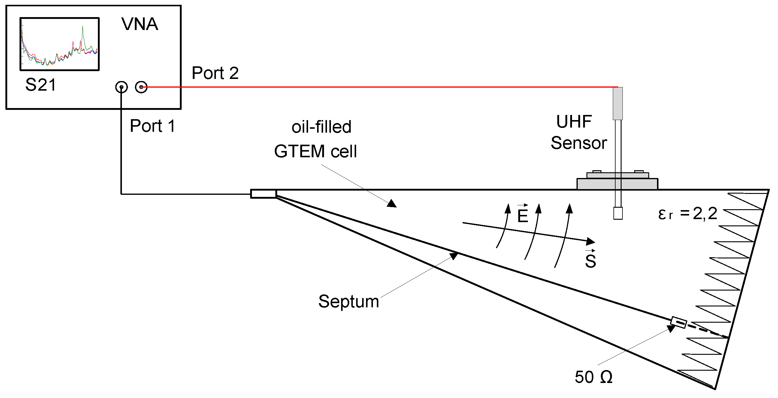
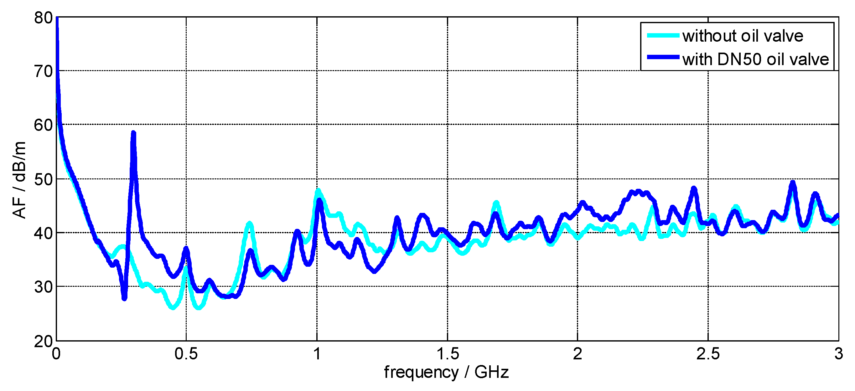
3.1. Measuring Technique

Electrical PD-measurement according to IEC 60270 [2] usually has sensitivity limitations for onsite/online measurements because of high noise levels in field. The “UHF PD measuring method” is based on the fact, that PD under oil are very fast electrical processes which radiate electromagnetic waves with frequencies in the ultrahigh range (UHF: 300–3000 MHz). Due to the moderately attenuated propagation of UHF signals inside the transformer, the sensitivity to electromagnetic wave detection is good [5,6,7,8]. UHF sensors, as shown in Figure 2, can be installed at the transformer during full operation through the oil filling valve. As a result of electromagnetical shielding characteristics of the grounded transformer tank against external disturbances, a clear decision can normally be made about the internal PD activity of the transformer under test.

When electrical or UHF PD measurements record PD activity, a three dimensional localization of PD is the next step for risk evaluation. This can be performed based on arrival time measurement of acoustical PD signals [9] using piezo-electric sensors mounted on transformer tank walls [10]. However, acoustic PD signals are affected by distortion within the tank from the windings, core and supporting structures in the transit path. The solution is to use a combination of the two methods: Sensitive UHF PD signals to provide triggering for the averaging of acoustic PD signals for de-noising. By using averaged signals, the acoustic PD pulses remain constructively overlapped, whereas the background noise is averaged to nearly zero [9].

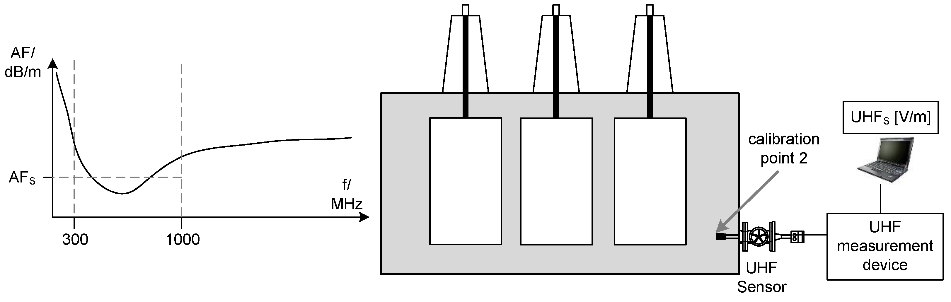
3.2. Calibration of Partial Discharge Measurements

The fundamental difference between the electrical PD measurement according to IEC 60270 [2] and the unconventional UHF PD measurement is their physical values. The apparent charge level in terms of picocoulomb (pC) of the electrical measurement is determined by integration of the recharging current. The electromagnetic radiation of the PD is measured in terms of millivolt (mV) using UHF sensors [11]. There is always a partly unknown propagation path because both methods cannot measure directly at the defect. Thus, the actual level of PD (pC or mV) remains unknown within a power transformer. Nevertheless, a common acceptance level for the apparent charge in terms of pC has become widely accepted, especially in factory acceptance tests (FAT). Due to disturbances by ambient noise and existing corona discharge activities, there are certain drawbacks for the use in the field or for online monitoring purposes. In theory, both measured variables contain the same information. A linear physical relation between measured UHF antenna voltage (in mV) and apparent charge (in pC) of the electrical measurement can be demonstrated in a constant laboratory setup with simple geometry [8]. However, it is not given for complex structures like power transformers. UHF antennas measure electromagnetic emissions of PD directly in oil inside a transformer tank, which acts as a “Faraday cage”. It becomes apparent that usually UHF measurement is advantageous regarding suppression of external disturbances. This makes it suitable for both, offsite measurement at routine tests under laboratory conditions with low ambient noise and especially onsite with usually high noise levels, e.g., after transportation and installation of transformers as a site acceptance test (SAT). These considerations make the UHF method interesting as supplement for transformer routine tests, when its sensitivity can be defined and demonstrated case by case. Both, the measureable electric and the electromagnetic PD levels, are influenced by the:

• type and actual level of the PD source;
• signal attenuation in the coupling path;
• sensor sensitivity (the UHF antenna or the coupling capacitor and the quadrupole);
• attenuation of the measurement cable and the sensitivity of the measurement device.

The influence of the electric setup (coupling capacitor and quadrupole) and the measurement device can be corrected using calibration for the electric measurement according to [2]. In order to determine the sensor sensitivity of the UHF sensor, its antenna factor (AF) must be known, which can be determined by means of an oil-filled gigahertz-transversal-electro-magnetic setup (GTEM) cell [12].

The sensitivity of an antenna depends on its design in relation to the electromagnetic wavelength. Antennas are usually described by different characteristic values, e.g., by the antenna gain or the antenna aperture. For antennas which are not defined by a physical area, such as monopoles or dipoles, the effective length l_eff or the AF can be used which is the following:

$$AF\left(f\right)=\frac{E(f)}{U(f)}$$

(2)

where U(f) is the voltage at the antenna terminals and E(f) is the electric field strength at the antenna.

An appropriate special designed oil-filled GTEM cell [12] is used for the evaluation of the antenna sensitivity. A GTEM cell is an expanded coaxial conductor where a defined electromagnetic field can be applied to the equipment under test (EUT) without interference from the ambient electromagnetic environment. In the cell, a test volume is defined in which the EUT is situated. In the test volume, the cell provides a homogeneous electric field distribution E_hom and an orthogonal magnetic field of the TEM wave, ideally. In addition, the electric field strength E_hom in the test volume has to be known for AF calculation of the EUT.

The AF of a UHF PD sensor can be measured using the transmission factor (S₂₁) (Figure 3). The measurement setup consists of the oil-filled GTEM cell with installed UHF sensor and the vector network analyzer (VNA). The sensor insertion depth should be the same like in the later field measurements; here an insertion depth of 50 mm from tank wall is used.

In this setup, the input port of the GTEM cell is excited with a sinusoidal frequency sweep from 300 kHz to 3 GHz generated by the VNA. The second port of the VNA simultaneously measures the resulting voltage at the output of the UHF sensor. The resulting transmission factor S₂₁ can be converted into the AF of the UHF sensor if the electric field strength in the test volume is taken into account. Two different AF of a UHF drain valve sensor are presented in Figure 4. Compared to a real transformer, the GTEM cell characterization measurement only considers the influence of the sensor and can therefore be regarded as first step reaching a calibration procedure.

To achieve a comparable method, UHF measurement systems require calibration including a validation of the UHF antenna sensitivity installed at the transformer. In a first step, a known UHF calibration impulse is injected into the measurement setup without antenna in order to calibrate the cable and the measurement device itself (Figure 5) [13].

From this calibration measurement, the calibration factor K₁ can be calculated:

$$K_1=\frac{U_0}{U_{\mathrm{m}}}$$

(3)

In a second step, the sensor’s characteristic is included into the calibrated path using its AF(f). The known transfer function provided by the AF allows the shifting of the calibration point from the injection point of the calibrator to the UHF antenna inside the transformer. In order to simplify the calibration procedure, the frequency dependent AF(f) can be reduced to a scalar correction factor AF_s which represents most common occurring UHF PD frequencies with sufficient accuracy. It is proposed to use the mean AF(f) from 300 MHz to 1 GHz as scalar.

$$A{F}_{\mathrm{s}}=\underset{300\text{MHz}\le \mathrm{f}\le 1\text{GHz}}{\text{mean}}AF(f)$$

(4)

The resulting AF_s can be used in its delogarithmized form K₂ to correct time domain signals.

$$K_2={10}^{\frac{A{F}_{\mathrm{S}}}{20}}$$

(5)

Figure 6 shows an example of simplifying the AF(f) to a mean AF_S and the new calibration point, which is shifted inside the transformer to the UHF antenna.

The idea of using a mean value of the frequency dependent AF(f) is only valid for broadband UHF measurement systems. When using a narrowband measurement system, the actual AF at the used center frequency should be used for K₂.

The complete UHF calibration factor K_UHF is calculated:

$$K_{\text{UHF}}=K_1\times K_2$$

(6)

An impulse U_m measured with the UHF measurement system can now be corrected and a value correlated to the electrical field emitted of a PD is displayed. This value can be called “apparent UHF signal” (UHF_S) similar to “apparent charge (q_S)” of the electrical PD measurement. It is called apparent as it is not directly related to the actual PD value itself but allows comparison of different measurement systems (including UHF sensors, cables and measuring devices) due to its calibration.

$$UH{F}_{\mathrm{S}}=K_{\text{UHF}}\times U_{\mathrm{m}}$$

(7)

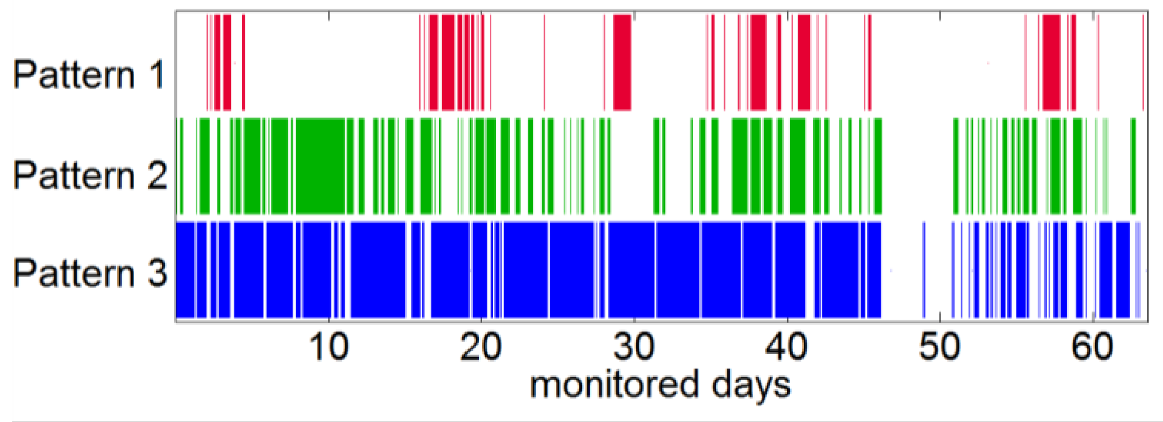
3.3. Online Monitoring of Partial Discharges

Online monitoring of power transformers, which supports established diagnosis methods, is steadily gaining importance. Continuous measurement and trend analysis allows to detect and trace undesirable changes at an early state. For PD, UHF monitoring represents an advantageous technique, because the measurement is done inside the tank and is thus much less sensitive to external noise. Additionally, it is applicable to transformers in service. The considerable amount of data generated requires appropriate evaluation; partially automated analysis is inevitable. A 50-year-old unit generator transformer with a rated voltage of 110/10 kV and a rated power of 120 MVA was monitored [14]. An online UHF PD measurement system recorded the UHF PD signals with 35 dB amplification and 9 MHz bandwidth at 505 MHz center frequency. Phase L1 was used for phase correlation. Due to the fact the generating unit is only in operation on demand, the transformer is not continuously in service. Measurements are available for approximately 65 days from 2009 to 2012. This case study presents an approach using phase-resolved PD pattern analysis. Typical patterns from known PD sources are reduced to an abstracted shape which uniquely characterizes the form of the PD source. This template is compared to measured phase resolved partial discharge pattern (PRPD) patterns gained from the monitoring data. Comparison between pattern and template is calculated by two-dimensional normalized cross-correlation algorithm. Source tracking over time is evaluated using continuous correlation. By introducing a set of templates for correlation, the progress of individual PD sources is determined.

Cross-correlation is an algorithm for recognition of patterns within images. The higher the similarity between two images, the higher is their correlation factor. In this contribution, the normalized cross-correlation is used providing values of correlation coefficients between −1 and +1 for each matrix element. Thus, cross-correlations of different images become comparable. A correlation coefficient of 1 indicates an exact match of the template (never occurs in practical pattern analysis), while −1 represents an area where image intersection and template are opposed (negative image, never occurs in practical pattern analysis). Figure 7 shows three typical PD patterns of this transformer.

Patterns should be traceable over time. Therefore, the constant PD data stream is divided into segments with constant duration. For each segment, a PRPD pattern is generated and then cross-correlated with the templates. Determining an adequate duration period depends on the behavior of the source over time. Pattern 1 from Figure 7 shows high volatility. Therefore, duration is set to one minute. The maximum value of the correlation matrix represents the correlation coefficient for the time segment. An example is plotted in Figure 8. The correlation coefficient is calculated by using a template which resembles a pattern as shown in Figure 7 (Pattern 1). The correlation coefficient is shown in red, aligned to the left axis. For comparison, the number of PD/min is plotted (black, right axis).

Figure 9 shows a bar graph for each pattern. Pattern 1 is only present 15% of the time showing intermitted behavior. Pattern 2 has a higher rate of appearance and can be detected 40% of the measurement time. Pattern 3 is the dominating source which can be detected 60% of the time over the entire period.

The essential benefit of the presented method is its application on very large PD datasets (e.g. from monitoring systems). In the case presented, 65 days of monitoring data were evaluated. Therefore, three PRPD patterns being typical for this specific transformer are evaluated. Using cross-correlation, it is possible to track patterns over the monitoring period in terms of their appearance and their phase positions.

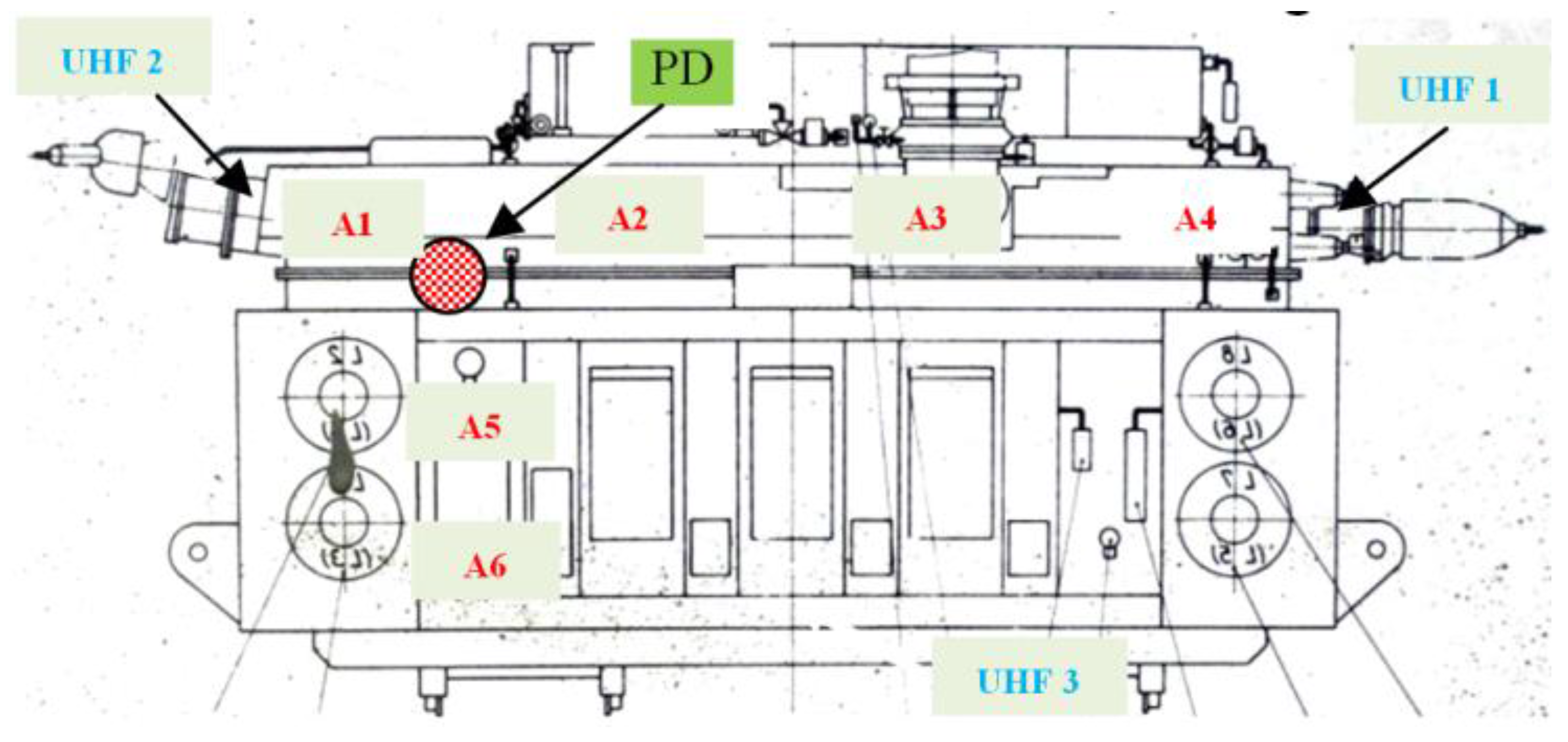
3.4. Localization of Partial Discharges

Because of increasing DGA values, a 333 MVA, 400/220kV single-phase autotransformer was tested onsite and online for PD. The high noise level in field strongly disturbed the electrical PD measurements made according to [2] at frequencies lower than 1 MHz. Source of noise was in that case the 400 kV bus bar above the transformer producing audible corona discharge [15].

Consequently, UHF PD measurements for PD detection were performed in combination with acoustic PD measurements for localization of the PD source in order to get reliable results. In this case, the transformer was equipped with three oil valves and therefore three identical UHF Sensors were installed. Figure 10 shows the positions of the UHF PD sensors (UHF 1–UHF 3) and the acoustic PD sensors (A1–A6).

At nominal voltage, UHF signals from internal PD sources were detectable with all three UHF sensors. The travelling speed of the electromagnetic waves is approximately 2/3 of speed of light inside the transformer. Thus, for localization, UHF signals are detectable almost the same time PDs occur. Conversely, the speed of acoustic waves is 1400 m/s, producing transit times within the range of milliseconds. With at least three acoustic sensors and corresponding time of flights, it is possible to calculate the intersection of the spheres and thus the PD location. It must be assumed that the acoustic waves travel directly in the line of sight from the PD source to the sensor without any reflections. Furthermore, the acoustical PD localization process also has to deal with acoustic waves travelling faster through the steel tank wall than through transformer oil. The time of flights of the acoustic signals can be computed accurately with the help of the Hinkley criterion [9], which is based on the signal energy of the measured signal [15].

As illustrated in Figure 10, the position of the located PD source is in the vicinity of the tap changer. Inaccuracy is thereby within the range of approx. 40 cm on all space axes. The time of flight differences were measured with six sensors, which are the three UHF sensors (UHF 1–UHF 3) and the three acoustic sensors (A2, A5, A6) placed near to the PD source [15].

After transportation of the transformer to the manufacturer the PD localization result was confirmed by an IEC triggered acoustic PD localization in a shielded test area and the transformer was detanked for repair. The visual inspection of the active parts at the tap changer confirmed the localization results. After repair procedure, the transformer passed the acceptance test without any indication of PD activity and was put back into service [15].

4. Frequency Response Analysis

Frequency response measurements are a widely applied technique for power transformer winding failure detection after lightning strike, short circuit or transport and are considered to be usually more sensitive than the conventional short-circuit voltage measurements [16]. Deviations between frequency responses indicate mechanical and/or electrical changes of the active part [17]. The basic principle of FRA is the investigation of differences between frequency responses. The electrical transfer behavior in the frequency range up to 2 MHz, in other words the frequency response, is identified by numerous characteristic resonances, which depend on the stray capacitances and inductances that are determined by the geometry and arrangement of active part and transformer tank [18]. The transfer function TF(f) as a state variable displays the geometric structural condition like a finger print. Known damage types, e.g., deformations, have an effect on the transfer functions like shifting, creating or disappearing of resonances [19]. However, interpretation of particular differences between two transfer function curves is the missing link between failure identification, measurement and assessment of the transformer. Figure 11 shows the frequency ranges with their corresponding winding parts being sensitive towards mechanical changes as identified by CIGRE WG A2.26 [20]. For smaller power transformers, the frequency ranges of interest tend to be shifted towards higher frequency.

4.1. Measuring Technique

The two most commonly used test types for transfer function measurement of power transformers are the so-called end-to-end transfer function measurement TF_EE(f) and the capacitive inter-winding (CI) measurement TF_CI(f) [20]. Figure 12 shows the associated connection diagrams. The obtained transfer function of a measured phase then is:

$${\underset{\_}{TF}}_{\text{EE}}\left(f\right)=\frac{{\underset{\_}{U}}_{2,\text{EE}}}{{\underset{\_}{U}}_1}$$

(8)

For the second measurement type, the transfer function is:

$${\underset{\_}{TF}}_{\text{CI}}\left(f\right)=\frac{{\underset{\_}{U}}_{2,\text{CI}}}{{\underset{\_}{U}}_1}$$

(9)

Each connection can be used for measuring the frequency response. However, some studies [21,22] showed that the inter-winding connections are more sensitive to common mechanical changes.

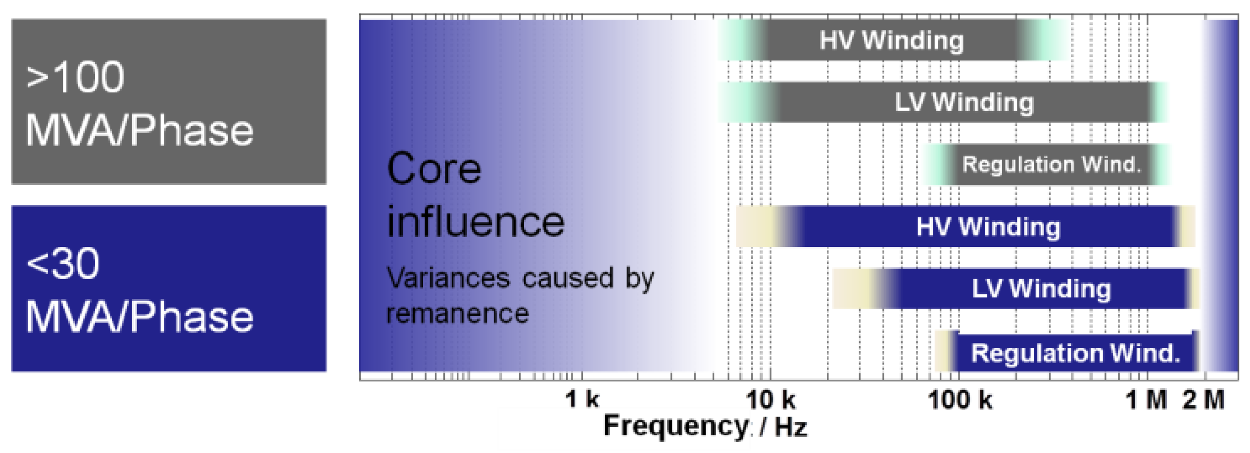
4.2. Influencing Factors

In addition to mechanical changes of the windings, other factors may also affect the frequency response of a transformer [23]. This may result in a false interpretation, i.e., an external factor influences the frequency response, but it is conceived to be a mechanical change. These factors are mainly the temperature, grounding practices, moisture contents, and shunt resistors [23,24]. The best situation occurs when two measurements are carried out in similar conditions, which requires that all of these factors be mentioned in the test sheet.

In order to explain misinterpretation, a case study is presented here. Figure 13 shows two traces of the middle phase of a 30 kVA/10 kV transformer measured at two different temperatures. The measurements were carried out on the same day and in a healthy condition. As can be seen, there are differences between these two traces. The amount of the difference extracted from these traces by numerical indices is approximately equal to that for 3 mm of axial displacement. As a result, this situation may be interpreted as a mechanical fault which is not the case. Other factors mentioned above may also change the frequency response and, therefore, special attentions should be paid to them during the measurement and the interpretation.

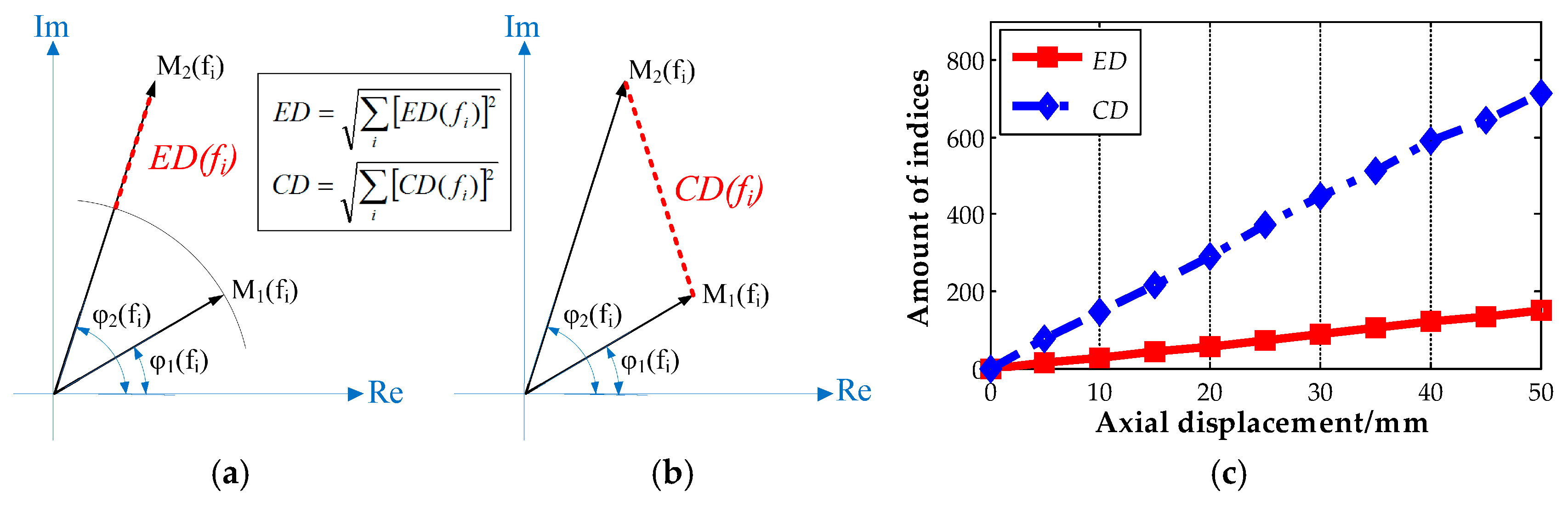
4.3. Interpretation of Frequency Response Measurement

The interpretation algorithms in the literature can be categorized into two main groups. In the first group, the transformer is modeled using circuit elements, and mechanical deformations are simulated by changing the values of these circuit elements [25,26,27,28]. After simulating different types and extents of mechanical deformations, comparison between the FRA traces extracted from the model with the one recorded from a real transformer can reveal the existence of a mechanical deformation in the transformer. In the second group, a numerical index is extracted from the FRA trace measured newly and the fingerprint. The interpretation, then, is carried out based on the values of indices [29,30,31,32,33,34].

Different amendments can be carried out regarding the interpretation; a case is mentioned here as an instance. Most of the numerical indices are based on only the magnitude response of the transfer function. However, the transfer function has a magnitude and a phase value in each frequency sample, i.e. a vector in the complex plane for each frequency sample, Figure 14. The index, Euclidean distance (ED) [24], calculates the magnitude differences of each frequency and, then, computes the root sum squared of them over the frequency range, Figure 14a. A new index, complex distance (CD), can be defined to include the phase information; it calculates the distance between two samples in the complex plane, Figure 14b,c shows the amounts of both indices for different steps of axial displacements in a winding. As can be seen, including the phase response does not impair the linearity of the index, but increases the sensitivity of the index to the mechanical change significantly, i.e., it makes the detection of the mismatches between two FRA traces simpler. Plenty of such works still need to be carried out to provide a reliable assessment algorithm for the FRA interpretation.

Figure 15 shows a representative case of transfer functions of all phases measured at a 200 MVA 110 kV/65 kV three phase power transformer. There are characteristic frequency bands that reflect different electrical properties of the transformer [33]. The lower frequency bands FB1 and FB2 are dominated by the core magnetizing inductance and winding series capacitance, while FB3 and FB4 are related to the leakage inductances of the windings and the capacitances of adjacent windings [36,37]. The high frequency part of FB4 up to 2 MHz represents smaller details of the active part geometry together with the winding leads. Additionally, the bushing capacitances influence the high frequency part of the transfer functions [38].

Differences between transfer functions of different phases are greater in FB1, FB2 and in the upper part of FB4. For FB1 and FB2, the differences can be explained by the unbalance of the core (magnetic circuit) and remanence of the core. Mismatching between phases in the upper part of FB4 can be explained by unbalances of the ground capacitances and the practical realization of the winding lead outs [39].

FB3 and the lower part of FB4 reflect the most important part of the frequency response. Deviations occurring in this frequency range indicate mechanical changes such as bulk winding movement or buckling of windings [33].

5. Dissolved Gas Analysis

The established DGA provides relevant information about internal transformer faults. Natural aging, thermal and electrical failures generate typical fault gases, which dissolve in the insulating oil. By analyzing these fault gas profiles evaluation of kind and severity of the fault can be estimated [40,41]. Usually, DGA assesses the severity of emerging faults using annually taken oil samples and evaluates both, ratios of different gases and long term gas generation rates [42]. The applicability of generation rates is enforced by the raising number of installed DGA monitoring systems, which provide continuous trend analysis [43]. The existing DGA standards are based on relatively complicated procedures, which can be well controlled under laboratory conditions. The field application with online monitoring systems, however, requires robustness and high long time precision for reliable trend development, which is the main focus of online monitoring.

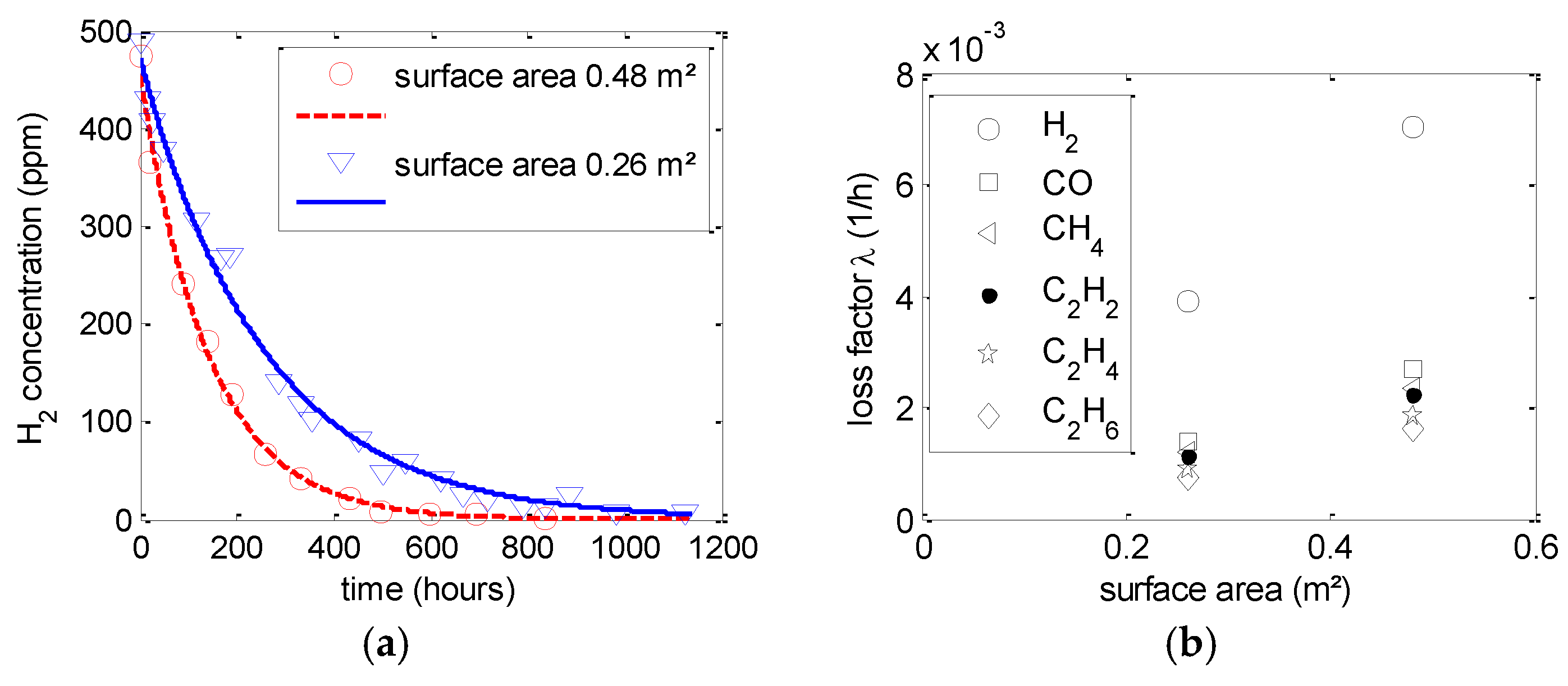
5.1. Dynamics between Oil and Gas Phase

A feasible gas based diagnosis requires the consideration of both, gas generation and gas losses. Gases escaping through the conservator tank may lead to misleading concentration levels and underrated gas generation rates especially for free breathing transformers [44]. In addition, the other way round is possible: gases from the ambient air, mainly nitrogen and oxygen, are slowly dissolving in the conservator tank oil and are afterwards mixed with the main tank oil, too [45]. An adequate model can help to assume the actual fault gas generation rate of a transformer. Thus, the severity of an upcoming fault could be determined more accurately for free breathing transformers. The loss of dissolved fault gases mainly depends on the conservator tank design. The oil is in direct contact to ambient air at free breathing conservator tanks. Fault gases can evaporate into the atmosphere and air gases can dissolve in the transformer oil. Free breathing conservator tanks for power transformers are common in several European and other countries [46]. Gas exchange does not occur at hermetically sealed transformers, transformers with a gas blanket or transformers with a membrane installed in the conservator tank.

The oil transports dissolved fault gases from the main into the conservator tank. There, the different fault gas concentrations between oil and air are equalized by diffusion, which results in a loss of fault gases and an increase of ambient air gases. Breathing depends on the exchange rate between main tank and conservator. The exchange rate depends on several factors: the entire oil volume of the transformer, the loading behavior of the transformer, the ambient temperature, the design of the conservator tank and its connection to the main tank. The oil flow is driven by two effects. The temperature dependent oil density forces a volume change of the oil and hence a flow from the main tank into the conservator tank at rising temperatures because oil expands with app. 0.076%/K. Additionally, a convection effect occurs (natural circulation), which is caused by the temperature gradient between main tank top oil temperature and the oil temperature in the conservator tank which approximately equals ambient temperature.

The flow rate for 26 different power transformers is calculated from thermal monitoring data in order to evaluate the effects of breathing [47]. The calculation only considers the oil flow due to volume change. The transformers’ nominal power varies between 31.5 MVA and 850 MVA including generator step-up units, grid couplers and wind park transformers. Therefore, the loading and the cooling types are diverse. The resulting flow rates cover a wide range from 4 L/day to 36 L/day per 1000 L oil volume for grid coupling and wind park transformers, both with volatile load factors. Generation step-up units provide a flow rate of 1.8–6.2 L/day per 1000 L oil volume, with stable load factors. Oil directed water forced (ODWF) units provide even lower flow rates because of a temperature controlled cooling system.

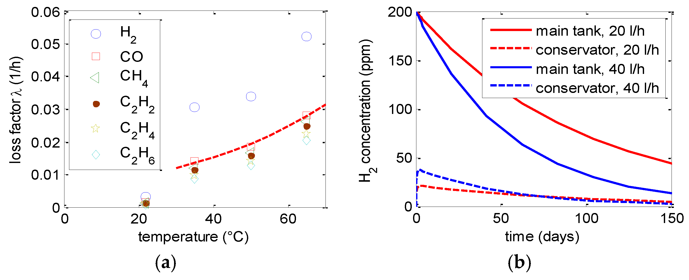
5.2. Gas Evaporation via Conservator

The exchange of gases at the boundary surface between oil and ambient air in the conservator tank is simulated in a laboratory setup. Barrels are used as substitutes for a conservator tank. These barrels have a total volume of about 217 L. To vary the surface area between oil and ambient air inside, one experiment is carried out with an upright standing barrel with a boundary surface of about 0.26 m² and one with a horizontal barrel and a boundary surface of about 0.48 m². The oil volume is kept constant at 100 (±5) L. Thus, there is a gas volume with about 117 L over the oil, which is open to the atmosphere. All experiments use mineral oil. Before each experiment, the oil is degassed, dried, and filtered at 60 °C with a vacuum oil treatment system. After degassing a fault gas mix is dissolved in the oil using a porous Polytetrafluoroethylene (PTFE) plastic.

The influence of the boundary surface between oil and ambient air on the loss of fault gases is examined by the two surface areas 0.26 m² and 0.48 m². The experiments are performed at room temperature. Throughout the experiment the oil is not moved. Figure 16a shows the concentration profile of hydrogen for the two different boundary surfaces. The curves are exponential partial regressions to the corresponding measured values, with C(t) = C₀ exp(−λt). The gas loss factor λ has the unit 1/h and depends on the boundary surface area.

The decrease of hydrogen concentration is faster for the larger surface area. Besides hydrogen, also other fault gases are analyzed with the same experimental setup. Figure 16b shows the gas loss factors λ of all gases for both surface areas. With a linear increasing surface area the gas loss factor also increases linearly. Thus, more gases evaporate. Hydrogen evaporates at the fastest rate, followed by CO and CH₄. C₂H₆ evaporates the slowest.

As the evaporation is also dependent on the influence of temperature, four different temperatures are investigated: room temperature (about 22 °C), 35 °C, 50 °C and 65 °C. All tests are performed using the same oil volume (100 L) and with a constant surface area between oil and ambient air (0.26 m²). Figure 17a shows the fitted gas loss factors λ for all gases at different temperatures. The gas loss factors over temperature show an exponential increase. An exemplary exponential gradient over temperature is plotted for CO. Again, H₂ has a higher gas loss factor and is more volatile than the other presented gases.

The large deviation between the gas loss factor at 22 °C and 35 °C may be explained by the experimental procedure. No heating of the test barrel is necessary at room temperature (22 °C). At higher temperatures (35–65 °C), a ring-shaped barrel heater is used. Due to the radial heat input a convection effect occurs in the oil. This leads to an increased mixing of the oil and thus to a higher gas loss factor.

5.3. Calculation of Fault Gas Losses

The conducted experiments show the possibility to calculate the gas losses of a free breathing conservator tank by taking the oil temperature and the boundary surface area into account. Changes of the gas concentration in the main tank influence the concentration in the conservator tank and vice versa. Therefore, the derivative of each concentration is affected by the concentrations of both, main and conservator tank.

A system of two differential equations is used for modeling the gas transport (Equations (10) and (11)).

$$\frac{\partial K\left(t\right)}{\partial t}=\mathrm{m}\times K(t)+\mathrm{n}\times A(t)$$

(10)

$$\frac{\partial A(t)}{\partial t}=\mathrm{p}\times A(t)+\mathrm{q}\times K(t)$$

(11)

where K(t) and A(t) are the time-dependent gas concentrations of the main tank oil K and of the conservator tank oil A, respectively; and m, n, p and q are constants that depend on the volume, the gas loss factor and the oil exchange rate.

The exemplary transformer has an oil volume of 42,000 L for the simulation. The free breathing conservator tank of this transformer has an oil filled volume of 1700 L. The main tank contains a concentration of 200 ppm dissolved hydrogen as starting condition. At the beginning, there is no dissolved hydrogen in the conservator tank. The exchange between the main and conservator tank is assumed constant at 20 L/h (40 L/h) corresponding to the results shown in Section 5.2. Every hour, 20 L oil flow into the conservator and back into the main tank. Temperatures are also considered constant. The gas loss factor in the conservator tank is set to λ_H2 = 0.1, which corresponds to a surface area of 1.5 m² and an average temperature of 15 °C. The λ_H2 value is extrapolated from the values measured in the experiment presented above.

Figure 17b shows the concentration trend for hydrogen with the previously made assumptions. The oil concentration of hydrogen in the main tank decreases exponentially. The concentration in the conservator first increases and then decreases exponentially. At a starting concentration for H₂ of 200 ppm the loss corresponds to 0.086 ppm/h or 2.06 ppm/d for an oil exchange of 20 L/h. At higher oil exchange rates, the losses also rise. The comparison between the calculations for 20 L/h and 40 L/h shows, that the fault gas loss is strongly influenced by the exchange of oil between main and conservator tank. For an improved model further laboratory tests as well as the evaluation of existing measurements from real transformers have to be performed.

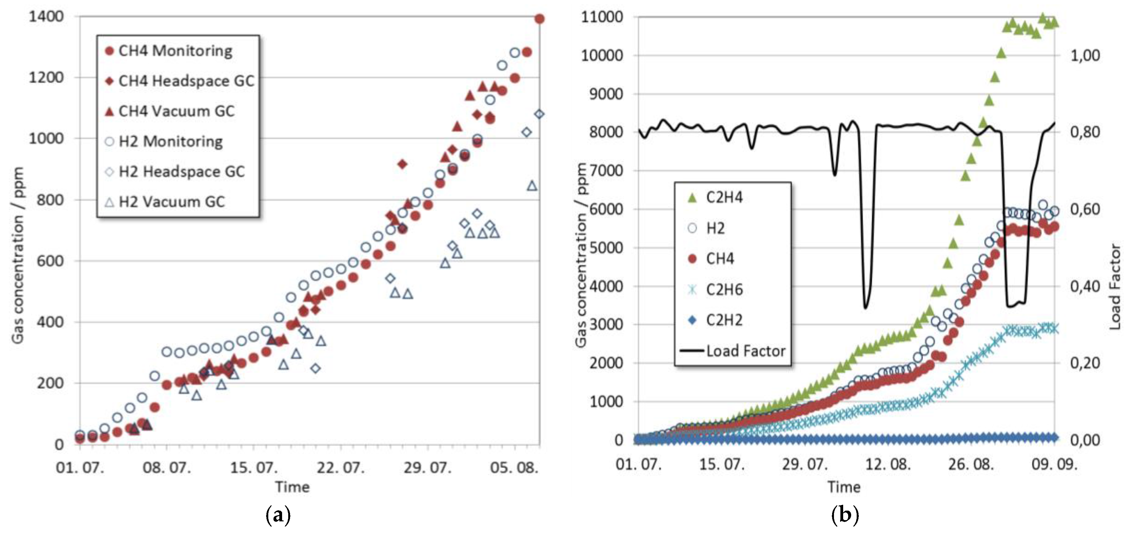
5.4. Online Monitoring of Fault Gases

A 600 MVA/380 kV generator step-up unit monitored by an IR-based multi gas analyzer showed in the beginning of July a strong and continuous increase of dissolved combustible gases (Figure 18). Because of the high TDCG rate (total dissolved combustible gases) of more than 100 ppm/day, in parallel to the DGA monitoring system oil samples were analyzed in the laboratory daily. This offered the possibility to check the deviation between monitoring and laboratory results. The dissolved gas was extracted by headspace and vacuum technology. Hydrocarbons showed very good agreement between monitoring and laboratory values (Figure 18a). The highest deviations occurred with hydrogen, which could be attributed to its high diffusivity. However, even though the oil samples analyzed in the laboratory revealed slightly different absolute gas values, the failure cause and trend corresponded fairly well with the monitoring results.

Most notably hydrogen, methane, ethane and ethylene were generated in high amounts. The Duval triangle indicated a thermal fault with temperatures above 700 °C. The concentration of CO and CO₂ stayed almost constant, which indicated no involvement of paper in the fault. Because the amount of acetylene increased during the first 50 days quiet slowly just by approximately 15 ppm melting of the core laminations was also excluded as failure cause.

In the beginning of August, the total amount of dissolved combustible gases (approximately 5000 ppm) and respective generation rate exceeded the values given as “Condition 4” according to IEEE Std C57.104 [42], which suggests to remove the transformer from service under these circumstances. Despite of the high dissolved combustible gas amounts (Figure 18b) no undissolved gases could be detected in the Buchholz relay. Additionally, the very low level of acetylene led to the decision to keep the transformer in service until a spare transformer would be in place. If the rise of acetylene had exceeded 5 ppm/day in an interval of two days or an abrupt rise of 5 ppm/h occurred, the transformer would have been switched off immediately. Due to the continuous monitoring of the different fault gases, this strategy of supervised extension of operation was possible in order to prevent switching off the power station with its high financial impact.

The reduction of load factor showed a stagnation of the gas generation. Based on the DGA results as potential failure causes problems with current leads (e.g., increased resistance of selector contacts or crimped connections) or circulating currents were taken into account. Unfortunately the repetitive changing of tap positions did not change the gassing behavior. After a further increase of the gassing rate the loading of the transformer was reduced by 50%. Due to this load reduction, the gas production stopped immediately, which at least could be interpreted as a temporary intermission of the failure. The following load increase also showed no resumption of the failure.

On 10 September 2012, the transformer was switched off as scheduled and exchanged by a spare unit provided at the time. A visual inspection of the tank revealed that due to mechanical problems the tank got in contact with the magnetic core sheets, which resulted in circulating currents via the normal core grounding system. This circulating current is induced by the load dependent stray flux and can reach levels of some hundred amperes. At the contact point of tank and core a hot spot with oil carbon was visible indicating the decomposition of the oil. Additionally, the copper cable for the normal grounding of the core outside on top of the tank was melted, which led to the intermission of the failure.

With this example of a large generator step-up transformer it is shown how the careful attention of the dynamic fault gas development offers the possibility to keep a faulty transformer longer in service. This enables the utility to keep the power station longer in operation in order to provide a spare transformer.

6. Moisture Measurement

6.1. Motivation

Moisture is a critical parameter of the insulating system for several reasons. One is that the dielectric strength of insulating liquid is strongly affected by moisture. The risk of PDs and the bubble effect (evaporation of water vapor under high load conditions) is higher. Water is also hazardous to the cellulose based insulation as it accelerates further ageing. Thus, by knowing the water content of a transformer's solid insulation it is possible to get an idea of its ageing condition and thus plan further actions.

The first source of water in the lifetime of a transformer can be from improper drying in the factory. Another can be moisture ingress from the atmosphere. This can happen for free-breathing transformers if the air-drying system is poorly maintained. Another source is during repair in the field where there are no possibilities of dry storage. The last, if not the most important one is moisture originating from ageing of paper and pressboard. This means that even a perfectly serviced transformer will become wet with increasing age. There are studies which show that the ageing accelerates with higher moisture content and at the same time water is produced due to ageing (Figure 19) [48]. One can conclude that lifetime estimations of cellulosic insulating systems do not only depend on operating temperature but also on moisture content of solid insulation. This is the reason why water assessment in combination with other diagnostic techniques can help finding the health condition of a transformer.

6.2. Methods of Moisture Assessment

The aim is to know the water content of the critical solid insulation which is the thin paper. It is nearly impossible to measure this directly as the paper cannot be sampled for measurement without destroying it. Here only indirect methods can help. Basically there are two groups of techniques: first are the moisture equilibrium charts and second are the dielectric response measurements. The equilibrium diagrams use the fact that the moisture in the paper-oil system reaches an equilibrium and will be distributed between oil and paper. Thus, by knowing the temperature and water content of the oil, one can estimate the water content in the solid. If the thermal and kinetic equilibrium cannot be guaranteed, these charts can give erroneous estimations additionally to sources of error during oil sampling and measurement in the laboratory [49].

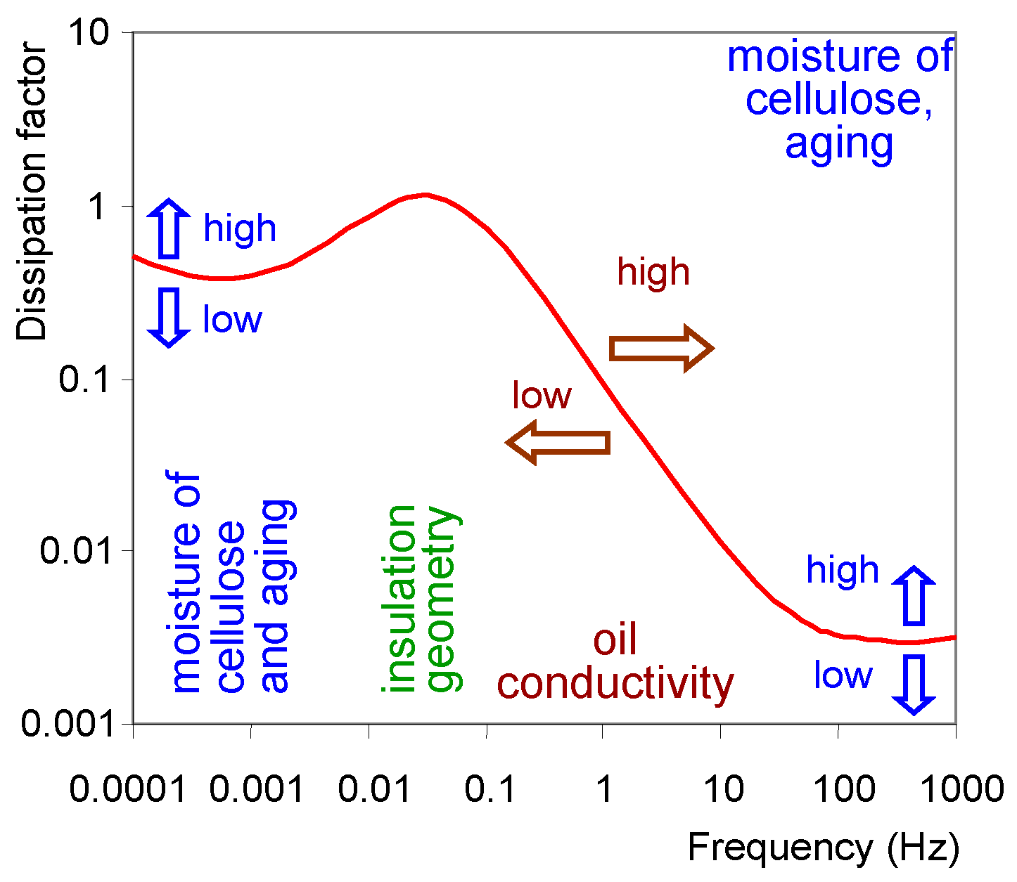
6.3. Dielectric Response Methods

Dielectric diagnostic methods assess moisture in paper or pressboard from dielectric properties like return voltage, polarization and depolarization currents (PDC) and dissipation factor. A time domain current measurement records the charging and discharging currents of the insulation. They are usually called PDC. FDS are derived from dissipation factor measurements, yet with a frequency range particularly enhanced for low frequencies. Figure 20 shows the typical s-shaped curve of the dissipation factor via frequency and the scientifically agreed interpretation scheme for a power transformer.

The transformer under investigation has to be offline. The dielectric response of the oil-paper system should be measured between HV and low voltage (LV) winding. On one side a variable frequency voltage source is connected and on the other winding the resulting current is recorded. With this information the loss factor can be calculated. These currents are very low and can easily be disturbed in the field. One protective means onsite is guarding, which avoids surface currents over the bushings from LV to HV. These fault currents would impede the measurement of the correct dielectric response and thus make the water assessment difficult.

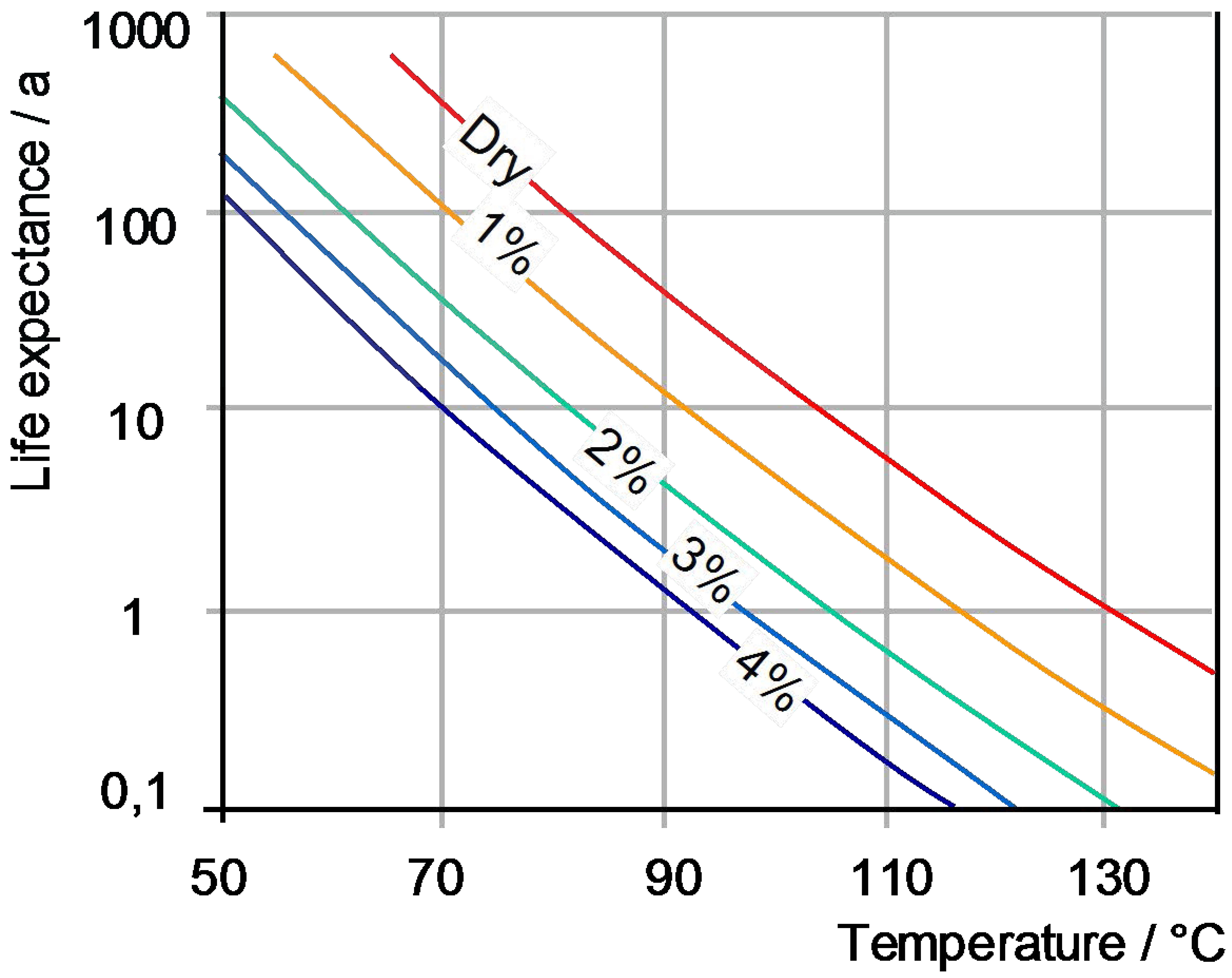
7. Thermal Monitoring for Life Estimation and Dynamic Rating

7.1. Advanced Thermal Model

As dynamic thermal models are used in most online monitoring system applications, their empirical verification, statistical evaluation and fundamental development are of key importance [51,52]. Thermal models are based on the modeling of heat transfer phenomena from top of the tank to the ambient with simple equations. However, their accuracy is limited in some cases because they consider the thermal resistance of a transformer as a constant value. Therefore, there is a need to improve the accuracy of these models with a more accurate determination of the thermal resistance.

An advanced thermal model is used to calculate the top-oil temperature which is based on IEC 60076-7 model [53]. The thermal-electrical analogy of the model is shown in Figure 21. The thermal resistances of this model are temperature dependent values and affected by the bottom-oil temperature and the temperature of the oil in the cooler [54].

In order to use a physical thermal model in an online monitoring system, the performance and accuracy of the model should be firstly validated. The model is applied on an oil directed air forced (ODAF) transformer whose main characteristics are listed in

Table 3. Characteristics of the transformer under study. ODAF: oil directed air forced.

Characteristic	Value	Characteristic	Value	Characteristic	Value
Power (MVA)	333	Mass of active parts and tank (to)	200	Number of Fans	8
Short circuit losses (kW)	510	Mass of oil (to)	50	Number of pumps	4
No load losses (kW)	47	Thermal capacitance (W·s/K)	199,050	Cooling system	ODAF

. For this transformer, the model has been parameterized using a dataset measured in June 2001, from beginning to the end of the month, during normal operation of the transformer. However, for validation of the model, the dataset measured in July 2001, from beginning to the end of the month, is used. The measured and calculated top-oil temperature using the advanced thermal model, load factor, ambient temperature, and number of running pumps and fans in July, from beginning to the end of the month, is illustrated in Figure 22a.

In order to compare the performance of the advanced thermal model with the model proposed in IEC 60076-7 [53], the error duration curve of each model is used which is shown in Figure 22b. The error duration curve shows the sorted absolute error dependent on the per cent time duration inside the observation time-window. As can be seen, the advanced thermal model represents better performance compared with IEC 60076-7 model for the calculation of the top-oil temperature. Due to the accuracy and simplicity of the advanced model, it can be used in an online monitoring system for monitoring of the cooling system and calculation of the overload capability of transformers.

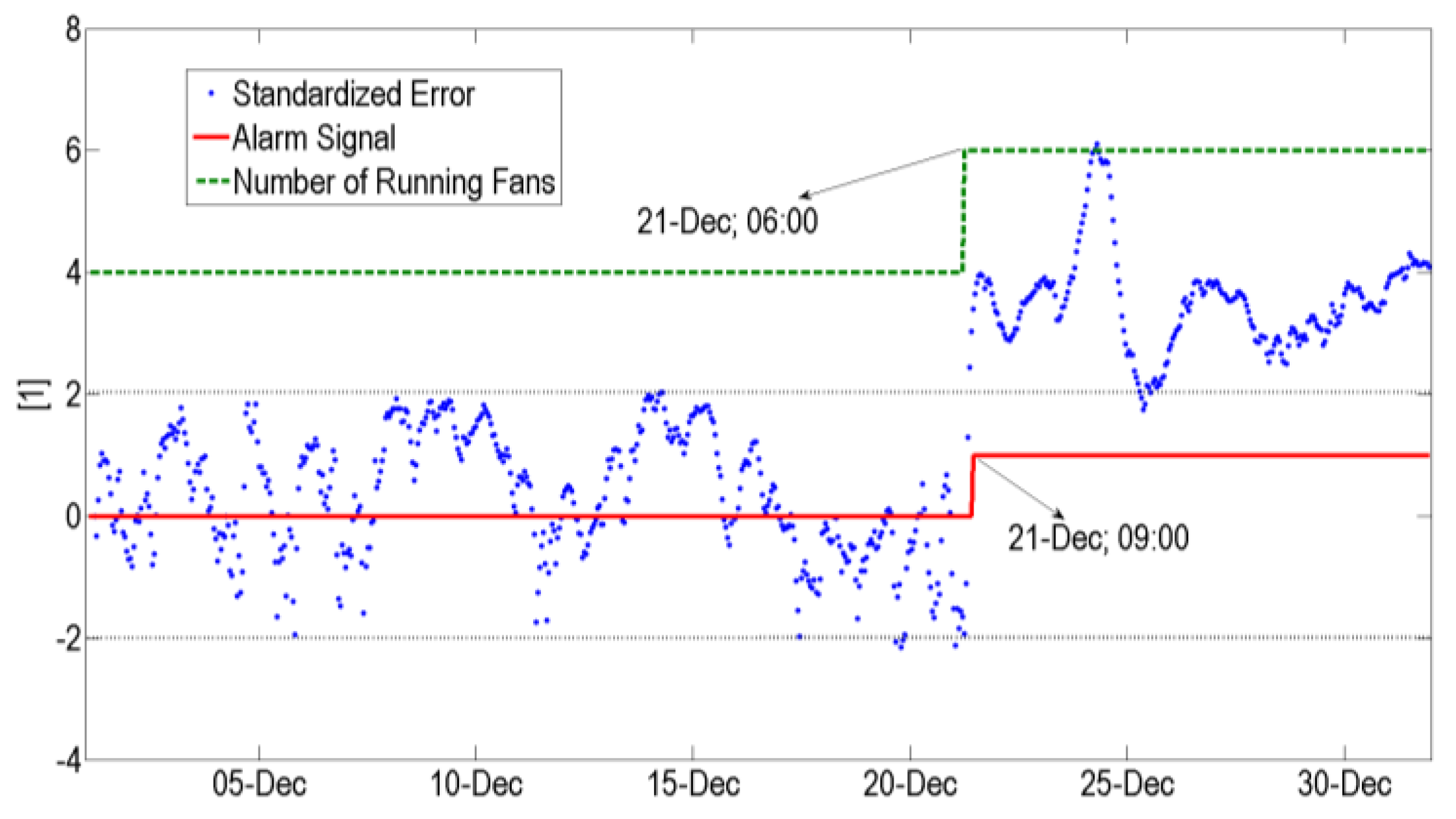
7.2. Monitoring of Cooling Unit

The transformer as described in Table 3 experienced a malfunction in a part of its cooling system due to a failure of the power supply which was not in accordance with the information supplied by the control system. The failure occurred on 21 December 2001 at 6:00 a.m. when the control system aimed to switch on two additional fans in order to reduce the oil temperature. However, due to the failure in the power supply of the fans, they did not start to run. The site check revealed later that two out of eight fans failed to operate while the pump related to the failed fans kept in operation.

The faulty operation of the cooling system can be detected based on a proper online algorithm for analysis of the deviation of the calculated top-oil temperature from the measured top-oil temperature [53,55]. Figure 23 shows the alarm signal of the monitoring system, the number of running fans provided by the control system, and the standardized error between the calculated and the measured top-oil temperature for the described malfunction of the fans. As can be seen, after failure of the two fans, the calculated temperature starts to deviate from the measured temperature indicating that a failure occurred in the cooling system. The standardized error exceeds the maximum allowable value leading to an alarm on 21 December 2001 at 9:00 a.m. In other words, the failure in the cooling system is detected 3 h (three steps) after the occurrence. Therefore, online thermal monitoring provides the ability to detect a malfunction of the cooling system with a short response time.

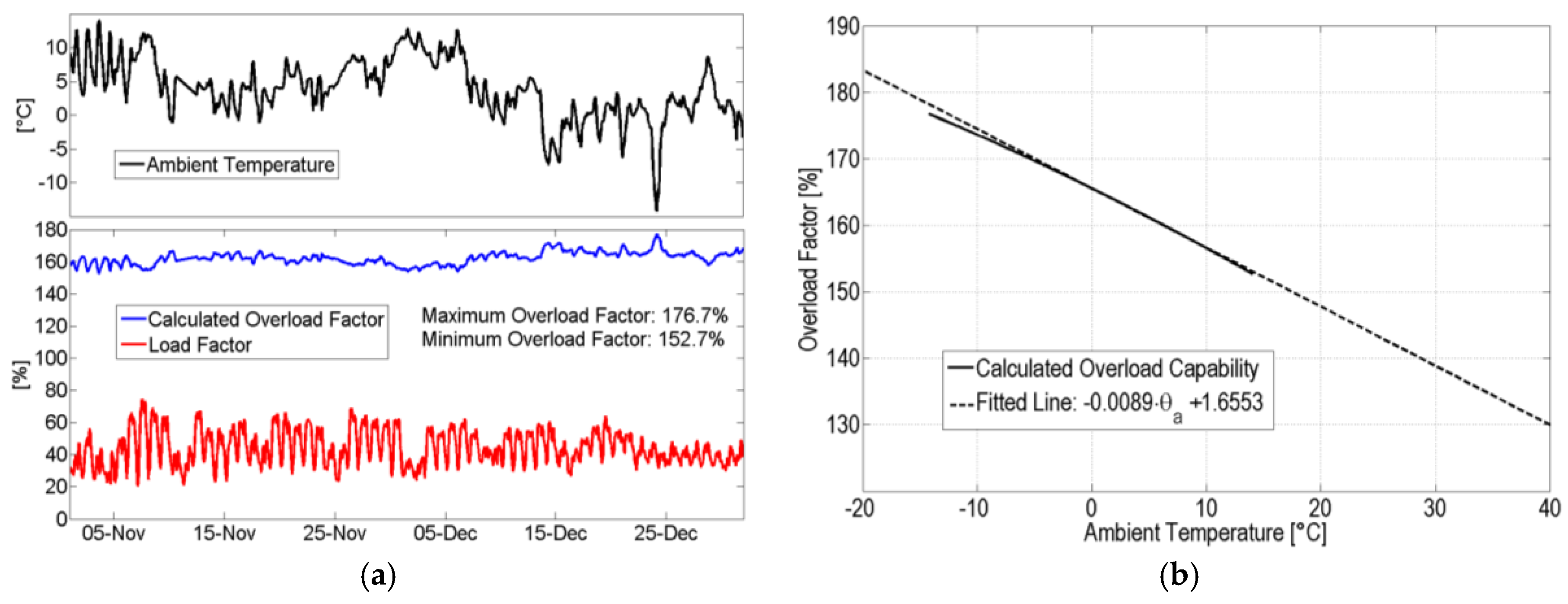
7.3. Assessment of Overload Capability

According to [53], a higher-than-rated load may be applied, but regarding the relative thermal ageing rate this loading should be equivalent to the rated load at normal ambient temperature (40 °C). This is achieved by taking advantage of low ambient temperatures during the rest of the load cycle. In other words, long-term overloading can be achieved as long as the hot spot temperature of the transformer does not exceed the allowed hot spot temperature corresponding to unity relative aging rate whose value for non-thermally upgraded paper is 98 °C.

Thus the hot spot temperature is the key word for the calculation of the overload capability of the transformer. The hot spot temperature Θ_hs is calculated using the top-oil temperature Θ_to as follows [53]:

$${\Theta }_{\text{hs}}={\Theta }_{\text{to}}+H\times g_{\mathrm{r}}\times k^y$$

(12)

where H is the hot spot factor. For medium and large power transformer, the value of H = 1.3 can be considered [53]. By solving this equation for the load factor k the long term overload capability of transformer is calculated considering that the hot spot temperature should not exceed 98 °C. It is assumed that the full cooling power of the transformer is in operation. Therefore, the overload capability OV depends only upon the ambient temperature Θ_a. This dependency can be written as a linear equation [56]:

$$OV=a\times {\Theta }_{\mathrm{a}}+b$$

(13)

Figure 24a illustrates the load factor, ambient temperature as well as the overload capability of the transformer according to Table 3. Of course, the loading capability of the transformer is increased at low ambient temperature. The dependency of the overload capability on the ambient temperature is depicted in Figure 24b. It should be noted that the cooling unit is an over-dimensioned by 33%, because two out of eight fans of this transformer are spare fans, which cause a very high overload capability at low ambient temperature and even at the nominal ambient temperature of 40 °C. However, limitations concerning other parts of a transformer, e.g., bushings and On-load tap changer (OLTC) during overloading periods, should also be kept in mind.

8. Conclusions

PD-measurement set-up according to [2] often has sensitivity limitations in case of onsite/online measurements because of the high noise level in field. UHF PD measurements can easily support PD measurements even online and are mostly sensitive enough against PD. As a result of shielding characteristics of the transformer tank against external electromagnetic waves, a clear decision can normally be made concerning the PD activity of the test object. A calibration procedure for the UHF method is proposed as it is necessary to ensure reproducibility and comparability of UHF measurements. Acoustic PD measurements for localization purposes should not be used exclusively and benefit from a sensitive trigger method as, e.g., UHF for double checking and noise suppression.

FRA is a helpful diagnostic tool when clearing up transformer failures after short circuit events or drop out after lightning strokes. Time-based comparison of frequency responses of a certain transformer unit promises most reliable assessments, as design-based or type-based comparisons are always critical due to natural unbalances between phases in design and inaccuracies of the production process.

The established DGA provides relevant information about internal transformer faults. A feasible gas based diagnosis for free breathing transformers requires the consideration of both gas generation and gas losses. An adequate model can help to assume the actual fault gas generation rate of a transformer. Thus, the severity of an upcoming fault could be determined more accurately for free breathing transformers.

Dielectric response methods deliver reliable results about the moisture condition of a transformer. They can be applied onsite even under conditions where the equilibrium state cannot be guaranteed. Disturbances can be reduced by proper connections and guarding.

An improved thermal model which takes the temperature dependency of thermal resistances into account allows thermal monitoring with a high accuracy. Thus, overloading capabilities dependent on ambient temperatures can be determined. During overloading periods, the cooling system of a power transformer plays a decisive role in transferring the heat generated in the windings to the surrounding ambient. Faulty operation of the cooling system can be detected by the proposed algorithm with a short response time.

The broadness and improvements of the presented diagnostic techniques show that the power transformer is no longer a black box that does not allow a view into its internal condition. Reliable and accurate condition assessment is possible leading to more efficient maintenance strategies.

References

1. Chakravorti, S.; Dey, D.; Chatterjee, B. Recent Trends in the Condition Monitoring of Transformers; Power Systems Springer-Verlag: London, UK, 2013. [Google Scholar]
2. IEC 60270. High-Voltage Test Techniques–Partial Discharge Measurements; International Electrotechnical Commission: Geneva, Switzerland, 2000. [Google Scholar]
3. Tenbohlen, S.; Jagers, J.; Vahidi, F.; Bastos, G.; Desai, B.; Diggin, B.; Fuhr, J.; Gebauer, J.; Krüger, M.; Lapworth, J.; et al. Transformer Reliability Survey; Technical Brochure 642 CIGRE: Paris, France, 2015. [Google Scholar]
4. Tenbohlen, S.; Jagers, J.; Bastos, G.; Desai, B.; Diggin, B.; Fuhr, J.; Gebauer, J.; Krüger, M.; Lapworth, J.; Manski, P.; et al. Development and Results of a Worldwide Transformer Reliability Survey. In Proceedings of the CIGRE SC A2 Colloquium, Shanghai, China, 20–25 September 2015.
5. Gulski, E.; Strehl, T.; Muhr, M.; Tenbohlen, S.; Meijer, S.; Judd, M.D.; Bodega, R.; Lemke, E.; Jongen, R.A.; Coenen, S.; et al. Guidelines for Unconventional Partial Discharge Measurements; Technical Brochure 444; CIGRE: Paris, France, 2010. [Google Scholar]
6. Judd, M.D. Experience with UHF Partial Discharge Detection and Location in Power Transformers. In Proceedings of the Electrical Insulation Conference, Annapolis, MD, USA, 5–8 June 2011.
7. Fuhr, J. Benefits and Limits of Advanced Methods Used for Transformer Diagnostics. In Proceedings of the IEEE Electrical Insulation Conference, Montreal, QC, Canada, 31 May–3 June 2009.
8. Coenen, S.; Tenbohlen, S.; Markalous, S.M.; Strehl, T. Sensitivity of UHF PD measurements in power transformers. IEEE Trans. Dielectr. Electr. Insul. 2008, 15, 1553–1558. [Google Scholar] [CrossRef]
9. Markalous, S.M.; Tenbohlen, S.; Feser, K. Detection and location of partial discharges in power transformers using acoustic and electromagnetic signals. IEEE Trans. Dielectr. Electr. Insul. 2008, 15, 1576–1583. [Google Scholar] [CrossRef]
10. Sikorski, W.; Siodla, K.; Moranda, H. Location of partial discharges sources in power transformers based on advanced auscultatory technique. IEEE Trans. Dielectr. Electr. Insul. 2012, 19, 1948–1956. [Google Scholar] [CrossRef]
11. Venkatesan, S.; Stewart, B.G.; Judd, M.D.; Reid, A.J.; Fouracre, R.A. Analysis of PD in Voids Using Correlation Plots of RF Radiated Energy and Apparent Charge. In Proceedings of the International Conference on Solid Dielectrics, Winchester, UK, 8–13 July 2007.
12. Siegel, S.; Tenbohlen, S. Design of an Oil-filled GTEM Cell for the Characterization of UHF PD Sensors. In Proceedings of the International Conference on Condition Monitoring and Diagnosis (CMD), Jeju, Korea, 21–25 September 2014.
13. Coenen, S.; Siegel, M.; Luna, G.; Tenbohlen, S. Parameters influencing Partial Discharge Measurements and their Impact on Diagnosis. In Proceedings of the Monitoring and Acceptance Tests of Power Transformers CIGRE Session, Paris, France, 22–26 August 2016.
14. Müller, A.; Beltle, M.; Siegel, M.; Tenbohlen, S. Assessment of UHF PD Monitoring Data by Means of Pattern Recognition. In Proceedings of the 18th International Symposium on High Voltage Engineering, Seoul, Korea, 25–30 August 2013.
15. Coenen, S.; Tenbohlen, S. Location of PD sources in power transformers by UHF and acoustic measurements. IEEE Trans. Dielectr. Electr. Insul. 2012, 19, 1934–1940. [Google Scholar] [CrossRef]
16. Gomez-Luna, E.; Aponte Mayor, G.; Gonzalez-Garcia, C.; Pleite Guerra, J. Current status and future trends in frequency-response analysis with a transformer in service. IEEE Trans. Power Deliv. 2013, 28, 1024–1031. [Google Scholar] [CrossRef]
17. Tang, W.H.; Wu, Q. Condition Monitoring and Assessment of Power Transformers Using Computational Intelligence; Power Systems Springer-Verlag: London, UK, 2011. [Google Scholar]
18. Wang, Z.D.; Li, J.; Sofian, D.M. Interpretation of transformer FRA responses; Part I: Influence of winding structure. IEEE Trans. Power Deliv. 2009, 24, 703–710. [Google Scholar] [CrossRef]
19. Rahimpour, E.; Christian, J.; Feser, K.; Mohseni, H. Transfer function method to diagnose axial displacement and radial deformation of transformer windings. IEEE Trans. Power Deliv. 2003, 18, 493–505. [Google Scholar] [CrossRef]
20. Cigre, W.G. Mechanical Condition Assessment of Transformer Windings using Frequency Response Analysis (FRA); Brochure 342; CIGRE: Paris, France, 2008. [Google Scholar]
21. Jayasinghe, J.A.S.B.; Wang, Z.D.; Jarman, P.N.; Darwin, A.W. Winding movement in power transformers: A comparison of FRA measurement connection methods. IEEE Trans. Dielectr. Insul. 2006, 13, 1342–1349. [Google Scholar] [CrossRef]
22. Samimi, M.H.; Tenbohlen, S.; Shayegani Akmal, A.A.; Mohseni, H. Effect of different connection schemes, terminating resistors and measurement impedances on the sensitivity of the FRA method. IEEE Trans. Dielectr. Insul. 2016, unpublished work. [Google Scholar]
23. Reykherdt, A.A.; Davydov, V. Case studies of factors influencing frequency response analysis measurements and power transformer diagnostics. IEEE Electr. Insul. Mag. 2011, 27, 22–30. [Google Scholar] [CrossRef]
24. Samimi, M.H.; Tenbohlen, S.; Shayegani Akmal, A.A.; Mohseni, H. Effect of Terminating and Shunt Resistors on the FRA Method Sensitivity. In Proceedings of the International Power System Conference, Tehran, Iran, 23–25 November 2015.
25. Bagheri, M.; Phung, B.T.; Blackburn, T. Influence of Temperature and Moisture Content on Frequency Response Analysis of Transformer Winding. IEEE Trans. Dielectr. Electr. Insul. 2014, 21, 1393–1404. [Google Scholar] [CrossRef]
26. Mitchell, S.D.; Welsh, J.S. Modeling power transformers to support the interpretation of frequency-response analysis. IEEE Trans. Power Del. 2011, 26, 2705–2717. [Google Scholar] [CrossRef]
27. Darwin, A.W.; Sofian, D.; Wang, Z.D.; Jarman, P.N. Interpretation of Frequency Response Analysis (FRA) Results for Diagnosing Transformer Winding Deformation. In Proceedings of the CIGRE 2009 6th Southern Africa Regional Conference, Cape Town, South Africa, August 2009.
28. Rahimpour, E.; Tenbohlen, S. Experimental and theoretical investigation of disc space variation in real high-voltage windings using transfer function method. IET Electric Power Appl. 2010, 4, 451–461. [Google Scholar] [CrossRef]
29. Ghanizade, A.J.; Gharehpetian, G.B. ANN and cross-correlation based features for discrimination between electrical and mechanical defects and their localization in transformer winding. IEEE Trans. Dielectr. Electr. Insul. 2014, 21, 2374–2382. [Google Scholar] [CrossRef]
30. Karimifard, P.; Gharehpetian, G.B.; Tenbohlen, S. Determination of axial displacement extent based on transformer winding transfer function estimation using vector-fitting method. Eur. Trans. Electr. Power 2008, 18, 423–436. [Google Scholar] [CrossRef]
31. Heindl, M.; Tenbohlen, S.; Kraetge, A.; Krüger, M.; Velásquez, J.L. Algorithmic Determination of Pole-Zero Representations of Power Transformers’ Transfer Function for Interpretation of FRA Data. In Proceedings of the 16th International Symposium of High Voltage Engineering, Cape Town, South Africa, 24–28 August 2009.
32. Rahimpour, E.; Jabbari, M.; Tenbohlen, S. Mathematical comparison methods to assess transfer functions of transformers to detect different types of mechanical faults. IEEE Trans. Power Del. 2010, 25, 2544–2555. [Google Scholar] [CrossRef]
33. Heindl, M.; Tenbohlen, S.; Velásquez, J.; Kraetge, A.; Wimmer, R. Transformer Modeling Based on Frequency Response Measurements for Winding Failure Detection. In Proceedings of the 2010 International Conference on Condition Monitoring and Diagnosis, Tokyo, Japan, 6–11 September 2010; pp. 201–204.
34. Nirgude, P.; Ashokraju, D.; Rajkumar, A.; Singh, B. Application of numerical evaluation techniques for interpreting frequency response measurements in power transformers. IET Sci. Meas. Technol. 2008, 2, 275–285. [Google Scholar] [CrossRef]
35. Samimi, M.H.; Tenbohlen, S.; Shayegani Akmal, A.A.; Mohseni, H. Using the Complex Values of the Frequency Response to Improve Power Transformer Diagnostics. In Proceedings of the 24th Iranian Conference on Electrical Engineering (ICEE), Shiraz, Iran, 10–12 May 2016.
36. Abeywickrama, N.; Serdyuk, Y.V.; Gubanski, S.M. Effect of core magnetization on frequency response analysis (FRA) of power transformers. IEEE Trans. Power Deliv. 2008, 23, 1432–1438. [Google Scholar] [CrossRef]
37. Abu-Siada, A.; Hashemnia, N.; Islam, S.; Masoum, M.A.S. Understanding power transformer frequency response analysis signatures. IEEE Electr. Insul. Mag. 2013, 29, 48–56. [Google Scholar] [CrossRef]
38. Wang, M.; Vandermaar, A.J.; Srivastava, K.D. Transformer winding movement monitoring in service—Key factors affecting FRA measurements. IEEE Electr. Insul. Mag. 2004, 20, 5–12. [Google Scholar] [CrossRef]
39. Shintemirov, A.; Tang, W.; Wu, Q. Transformer winding condition assessment using frequency response analysis and evidential reasoning. IET Electr. Power Appl. 2010, 4, 198–212. [Google Scholar] [CrossRef]
40. Bakar, N.A.; Abu-Siada, A.; Islam, S. A review of dissolved gas analysis measurement and interpretation techniques. IEEE Electr. Insul. Mag. 2014, 30, 39–49. [Google Scholar] [CrossRef]
41. Möllmann, A.; Pahlavanpour, B. New guidelines for the interpretation of dissolved gas analysis in oil-filled transformers. Electra 1999, 186, 31–51. [Google Scholar]
42. IEEE Guide for the Interpretation of Gases Generated in Oil Immersed Transformers; IEEE Std. C57.104; IEEE Power & Energy Society: New York, NY, USA, 2008.
43. Report on Gas Monitors for Oil-filled Electrical Equipment; Cigré Technical Brochure 409; Cigre: Paris, France, 2010.
44. Anderson, R.; Roderick, U.R.; Jaakkola, V.; Östman, N. The Transfer of Fault Gases in Transformers and Its Effect upon the Interpretation of Gas Analysis Data; Cigré Report 12-02; Cigre: Paris, France, 1976. [Google Scholar]
45. Bräsel, E.; Bräsel, O.; Sasum, U. Gashaushalt bei Transformatoren der offenen Bauart—Neue Erkenntnisse; EW-Medien und Kongresse: Frankfurt, Germany, ew, Jg. 109, Heft 14–15; pp. 56–59. 2010. (In German) [Google Scholar]
46. Recent Developments in DGA Interpretation; Cigré Technical Brochure 296; Cigre: Paris, France, 2006.
47. Müller, A.; Tenbohlen, S. Analysis of Fault Gas Losses through the Conservator Tank of Free-Breathing Power Transformers. In Proceedings of the 18th International Symposium on High Voltage Engineering, Seoul, Korea, 25–30 August 2013.
48. Lundgaard, L.E.; Hansen, W.; Linhjell, D.; Painter, T.J. Aging of oil-impregnated paper in power transformers. IEEE Trans. Power Deliv. 2004, 19, 230–239. [Google Scholar] [CrossRef]
49. Koch, M.; Tenbohlen, S.; Stirl, T. Diagnostic application of moisture equilibrium for power transformers. IEEE Trans. Power Deliv. 2010, 25, 2574–2581. [Google Scholar] [CrossRef]
50. Koch, M.; Krüger, M.; Tenbohlen, S. Comparing Various Moisture Determination Methods for Power Transformers. In Proceedings of the CIGRE South Africa Regional Conference, Cape Town, South Africa, 17–21 August 2009.
51. Susa, D.; Lehtonen, M.; Nordman, H. Dynamic thermal modelling of power transformers. IEEE Trans. Power Deliv. 2005, 20, 197–204. [Google Scholar] [CrossRef]
52. Lesieutre, B.C.; Hagman, W.H.; Kirtley, J.L., Jr. An improved transformer top oil temperature model for use in an online monitoring and diagnostic system. IEEE Trans. Power Deliv. 1997, 12, 249–256. [Google Scholar] [CrossRef]
53. IEC 60076-7. Power Transformers—Part 7: Loading Guide for Oil Immersed Power Transformers; International Electrotechnical Commission: Geneva, Switzerland, 2005. [Google Scholar]
54. Djamali, M.; Tenbohlen, S. A Dynamic Top Oil Temperature Model for Power Transformers with Consideration of the Tap Changer Position. In Proceedings of the 19th International Symposium on High Voltage Engineering, Pilsen, Czech Republic, 23–28 August 2015.
55. Djamali, M.; Tenbohlen, S. Malfunction detection of the cooling system in air-forced power transformers using online thermal monitoring. IEEE Trans. Power Deliv. 2016, unpublished work. [Google Scholar]
56. Tenbohlen, S.; Djamali, M. A Dynamic Top-Oil Temperature Model for Online Assessment of Overload Capability of Power Transformers. In Proceedings of the CIGRE SC A2 Colloquium, Shanghai, China, 20–25 September 2015.
Figure 1. Failure locations of substation transformers (>100 kV) (based on 536 major failures) [4].
Energies 09 00347 g001
Figure 2. UHF PD probe for standard oil filling valve.
Energies 09 00347 g002
Figure 3. Transmission measurement (S21) for antenna factor (AF) determination [13].
Energies 09 00347 g003
Figure 4. AF of UHF sensor measured in gigahertz-transversal-electro-magnetic (GTEM) cell [13].
Energies 09 00347 g004
Figure 5. Calibration of measurement device and cables [13].
Energies 09 00347 g005
Figure 6. Calibration of the UHF sensor.
Energies 09 00347 g006
Figure 7. UHF phase resolved partial discharge patterns (PRPDs): (a) Pattern 1; (b) Pattern 2; and (c) Pattern 3 [14].
Energies 09 00347 g007
Figure 8. Number of PD per minute and correlation coefficient [14].
Energies 09 00347 g008
Figure 9. Results of recognition algorithm of determined Patterns 1–3 [14].
Energies 09 00347 g009
Figure 10. Positions of UHF and acoustic PD sensors and the localized PD source in a 333 MVA/400 kV single phase autotransformer [15].
Energies 09 00347 g010
Figure 11. Frequency ranges with known sensitivity towards changes of the winding geometry [20].
Energies 09 00347 g011
Figure 12. Connection schemes for measurements of end-to-end (EE) and capacitive inter-winding (CI) frequency response.
Energies 09 00347 g012
Figure 13. The middle phase frequency response of a three-phase oil transformer for two different temperatures. The traces correspond to the CI connection.
Energies 09 00347 g013
Figure 14. (a,b) The ith samples of the new and the fingerprint frequency response in the complex plane. M and ϕ corresponds to the magnitude and phase values of a sample; and (c) comparison of the two indices for different amounts of axial displacements [35].
Energies 09 00347 g014
Figure 15. Characteristic frequency bands of measured end-to-end frequency responses of a three phase power transformer [33].
Energies 09 00347 g015
Figure 16. (a) Concentration trend of hydrogen for different boundary surface areas; and (b) gas loss factor over surface area for different fault gases.
Energies 09 00347 g016
Figure 17. (a) Gas loss factors of different fault gases over temperature. Dashed line: exemplary exponential gradient for CO; and (b) concentration trend for H2 in main tank (straight line) and conservator (dashed line) at different oil exchange rates.
Energies 09 00347 g017
Figure 18. Development of gas concentration of a 600 MVA/380 kV GSU transformer: (a) first 5 weeks; and (b) 10 weeks.
Energies 09 00347 g018
Figure 19. Life expectance of oil impregnated paper depending on temperature and water content [48].
Energies 09 00347 g019
Figure 20. Interpretation of the dissipation factor vs. frequency of an oil-paper-insulation system [50].
Energies 09 00347 g020
Figure 21. Thermal-electrical analogy of the advanced thermal model [54].
Energies 09 00347 g021
Figure 22. (a) The calculated and the measured top-oil temperature during the normal operation of the transformer in July; and (b) the error duration curves of IEC 60076-7 and the advanced thermal model.
Energies 09 00347 g022
Figure 23. Standardized error between measured and calculated oil temperature for faulty operation of fans.
Energies 09 00347 g023
Figure 24. (a) Ambient temperature, long-term overload factor and load factor; and (b) dependency of overload capability on ambient temperature [56].
Energies 09 00347 g024