Three-Dimensional Finite-Element Analysis of the Short-Time and Peak Withstand Current Tests in Substation Connectors

Abstract

Power devices intended for high-voltage systems must be tested according to international standards, which includes the short-time withstand current test and peak withstand current test. However, these tests require very special facilities which consume huge amounts of electrical power. Therefore, mathematical tools to simulate such tests are highly appealing since they allow reproducing the electromagnetic and thermal behavior of the test object in a fast and economical manner. In this paper, a three-dimensional finite element method (3D-FEM) approach to simulate the transient thermal behavior of substation connectors is presented and validated against experimental data. To this end, a multiphysics 3D-FEM method is proposed, which considers both the connector and the reference power conductors. The transient and steady-state temperature profiles of both the conductors and connector provided by the 3D-FEM method prove its suitability and accuracy as compared to experimental data provided by short-circuit tests conducted in two high-current laboratories. The proposed simulation tool, which was proven to be accurate and realistic, may be particularly useful during the design and optimization phases of substation connectors since it allows anticipating the results of mandatory laboratory tests.

1. Introduction

It is a recognized fact that the world today is more electrical than a few decades ago. According to data compiled by the International Energy Agency [1], world electricity generation has almost quadrupled during the last four decades, and is continuing to grow. Due to the fast expansion of transmission systems worldwide, power networks are becoming more complex and dense. Short-circuit currents are increasing, thus increasing the risk of damage because they can exceed the breaking capacity of the electrical protections in the networks [2]. Since short-circuits in power systems can lead to severe faults [3], it is crucial to ensure that the fault currents are below the safety limits of the equipment involved. The occurrence of short-circuit faults leads to unusual temperatures of the components involved, since the electrical protections need some time to clear such fault currents [4].

Standard short-time withstand current tests and peak withstand current tests, commonly referred to as short-circuit tests, are applied to several electrical devices, including power transformers, switchgear, control gear and substation connectors, among others. Therefore, these standard tests are a subject of increasing interest, both in constructing improved facilities to perform such demanding tests, which include modern digital measuring systems [5], as well as in developing software tools to realistically simulate the performance of different power devices when subjected to short-circuit tests.

It is well-known that short-circuits generate thermal and electromechanical stresses [6,7], so power systems are designed and tested to ensure that the electrical and mechanical devices involved can withstand short-circuit conditions. To this end, such devices are tested and certified according to the short-time withstand current and peak withstand current tests, which are defined by different international standards [8,9,10].

Substation connectors are required to endure a short-time withstand current of some tens of kilo-amps, usually within 1 s [9], to ensure adequate behavior under short-circuit conditions. However, the thermal stress generated may increase the contact resistance, thus affecting contact stability [11] and therefore the expected service life, due to an increase of the power losses. Therefore, to ensure reliable operation, connectors should not suffer from excessive overheating during short-circuit conditions [12], thus their suitable thermal behavior must be ensured. Due to the huge current requirements in terms of instantaneous power [13], short-circuit tests must be carried out in very specific and expensive laboratory facilities, in which customers often have to face long waiting times. Therefore, short-time withstand current tests are expensive, due to the laboratory facilities required, time-consuming due to the laborious installation of the experimental setup, and destructive since the test object is usually rejected once tested.

An attractive and cost-effective solution is to use an advanced modelling tool to perform realistic simulations to determine the thermal stresses to which substation connectors are subjected during short-time withstand current and peak withstand current tests, from which the risk of increasing the contact resistance can be estimated. By using this modelling tool to assist the connectors’ design process, an optimized design can be achieved, thus satisfying the electromagnetic and thermal requirements imposed by international standards [14] and ensuring compulsory laboratory tests are passed once optimized. It is noted that there are some variables that are not considered in the FEM model, such as poor workmanship or use of low quality material.

Modelling the short-time withstand current test and peak withstand current test in substation connectors gives rise to a challenging multiphysics problem because electric, magnetic and thermal equations must be formulated and solved altogether. In this problem, the heat source is primarily due to the Joule’s losses caused by the main current and the induced eddy currents, and therefore, both skin and proximity effects must be taken into account. In addition, conductive, convective and radiative phenomena must be considered to accurately model the thermal behavior of the connector. Several authors have attempted to develop electromagnetic and thermal coupled mathematical formulations to model the temperature rise or the temperature distribution in different power devices such as power conductors and cables, bus bars, surge arresters or transformers [15,16,17,18,19,20,21,22,23] by means of two-dimensional (2D-) and three-dimensional finite element method (3D-FEM) approaches. Nevertheless, the abovementioned references do not analyze the problem under study, that is, the thermal analysis of the short-circuit test, although in [24] a transient 3D-FEM model to simulate the short-time withstand current capability of an air circuit breaker is presented. To the authors’ knowledge, no attempts have been made to model the electromagnetic and thermal behavior of substation connectors during the standard short-time and peak withstand current tests, which can be a fast and valuable tool to optimally design the thermal behavior of such power devices, especially useful during the design and optimization stages [14]. This paper proposes a multiphysics 3D FEM-based model to accurately determine the thermal behavior of complex-shaped electrical connectors during the short-time withstand and peak withstand current test, which has not yet been reported in the technical literature. The proposed model deals with heat transfer coefficients whose values are automatically adapted to the geometry of the connector and conductors, fluid properties such as density, viscosity or thermal conductivity and surface temperatures. It also calculates the transient temperature distribution in both the connector and the power conductors or bus bars to which the connector is linked. Finally, the results provided by the simulation tool are validated by means of experimental data. It is worth noting that, although the tool presented here is intended to simulate the performance of power connectors, the approach carried out can also be applied to many other types of power devices.

2. The Short-Time Withstand Current and Peak Withstand Current

According to IEC 62271-1:2007 Standard [9], the rated short-time withstand current, often denoted as I_k, is the root-mean-square (RMS) value of the current that the analyzed electrical device can withstand under specified conditions during a prescribed period of time. These standards also specify the rated duration t_k of the short-circuit as 1 s, although 0.5 s, 2 s and 3 s are also permitted for switchgear.

IEC and IEEE [9,25] also defined the rated peak withstand current, denoted as I_p, as the peak value of the first major loop (Figure 1) of the rated short-time withstand current which the electrical device under analysis can withstand under specified conditions. It must be selected according to the dc time constant (τ = L/R) of the loop under test.

It is worth noting that substation connectors and other electrical devices must be designed to safely withstand their associated rated short-time and peak withstand currents, that is, without causing any mechanical damage to their components. Although IEC 62271-1 Standard [9] does not specify any temperature limit for the short-time current withstand test, it states that the temperature rise of the test object must not be enough to produce significant damage, thus proving its thermal capability [25,26].

Therefore, the study of the short-time withstand current and peak withstand current tests is of great interest in low and high voltage applications, including vacuum and air circuit breakers [11,24,27] or transformers [5] among others, whose results are very valuable in order to optimize the design and behavior of such electrical devices [24]. The differential equation governing the creation of an R-L inductive loop is given by:

$$V_{\mathrm{o}}\sin (\mathsf{\omega }t+{\mathsf{\theta }}_{\mathrm{v}})=Ri(t)+L\frac{\mathrm{d}i(t)}{\mathrm{d}t}$$

(1)

The transient short-circuit current flowing through an inductive shorted loop can be written as [24]:

$$i(t)=\underset{\text{DC\hspace{0.17em}\hspace{0.17em}component\hspace{0.17em}\hspace{0.17em}term}}{\underbrace{I_0\sin ({\mathsf{\theta }}_{\mathrm{v}}-\mathsf{\varphi }){\mathrm{e}}^{-\frac{R}{L}t}}}-I_0\sin (\mathsf{\omega }t+{\mathsf{\theta }}_{\mathrm{v}}-\mathsf{\varphi })$$

(2)

where $I_0=V_{\mathrm{o}}/\sqrt{R^2+{(\mathsf{\omega }L)}^2}$ and ϕ = tg⁻¹(ωL/R). From Equation (2), it is deduced that by a tight control of the voltage phase angle θ_v during the making instant, the peak value of the transient short-circuit current can be changed from I₀ to 2I₀. For example, when θ_v = ϕ the DC component term in Equation (2) is null and thus the peak value of the current results in I₀. Conversely, when θ_v = ϕ + 90°, the dc term is maximum, and the peak value of the current is 2I₀. Figure 1 shows the short-circuit current as described by Equation (2).

3. The Analyzed Connectors

This paper analyzes by means of simulations and experimental laboratory tests the thermal behavior of a J33SPK two-cap coupler substation connector (Model A, SBI Connectors, Sant Esteve Sesrovires, Spain) made of A356.0 cast aluminum alloy from the catalogue of SBI-connectors, which is shown in Figure 2a. This coupler connects two 32 mm diameter Hawthorn all aluminum conductors (AAC, HAASE Gesellschaft m.b.H, Graz-Puntigam, Austria).

To further validate the coupled electromagnetic-thermal FEM model proposed in this paper, simulations are also conducted on a bimetallic terminal Class A for low- and medium-voltage applications, reference YAT450AM20C (Model B) from the catalogue of SBI-connectors, which is shown in Figure 2b. The connector is composed of Al 99.5% (barrel), and Cu 99.9% (palm). It connects two 450 mm² AA-8030 AL conductors.

The main characteristics of the analyzed connectors are summarized in

Table 1. Analyzed connectors. AAC: all aluminum conductors.

Model	Connector	Conductor	Parts	Material
A	Coupler substation connector (J33SPK)	Hawthorn AAC 604.2 mm2	AAC conductor	Aluminum
			Coupler connector	A356.0 alloy
			Bolts	Steel
B	Bimetallic terminal Class A (YAT450AM20C)	AA-8030 AL 450 mm2	AA-8030 AL Conductor	Aluminum
			Terminal’s barrel	Aluminum 99.5%
			Terminal’s palm	Copper 99.9%

.

4. The Three-Dimensional Finite Element Method Model

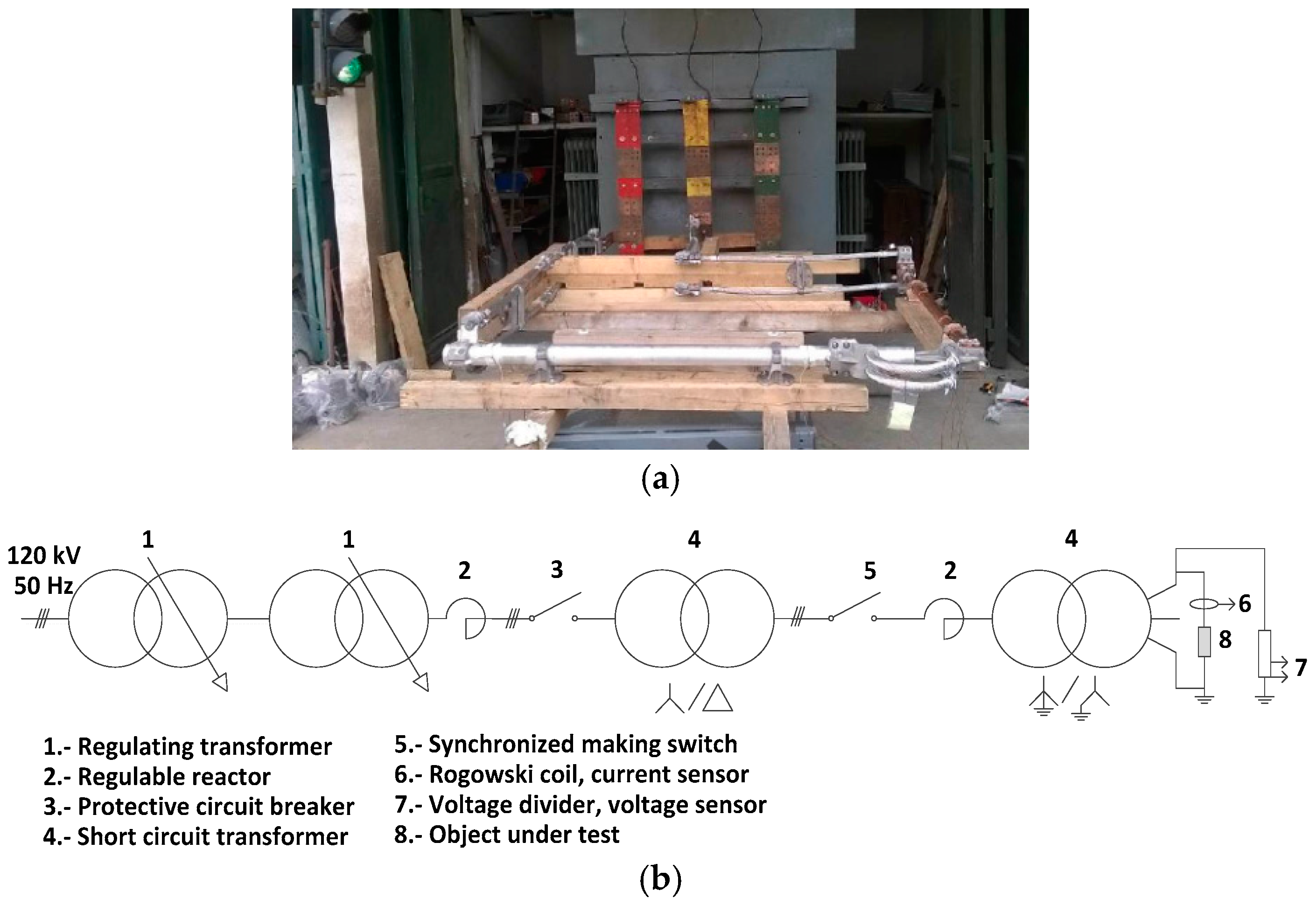
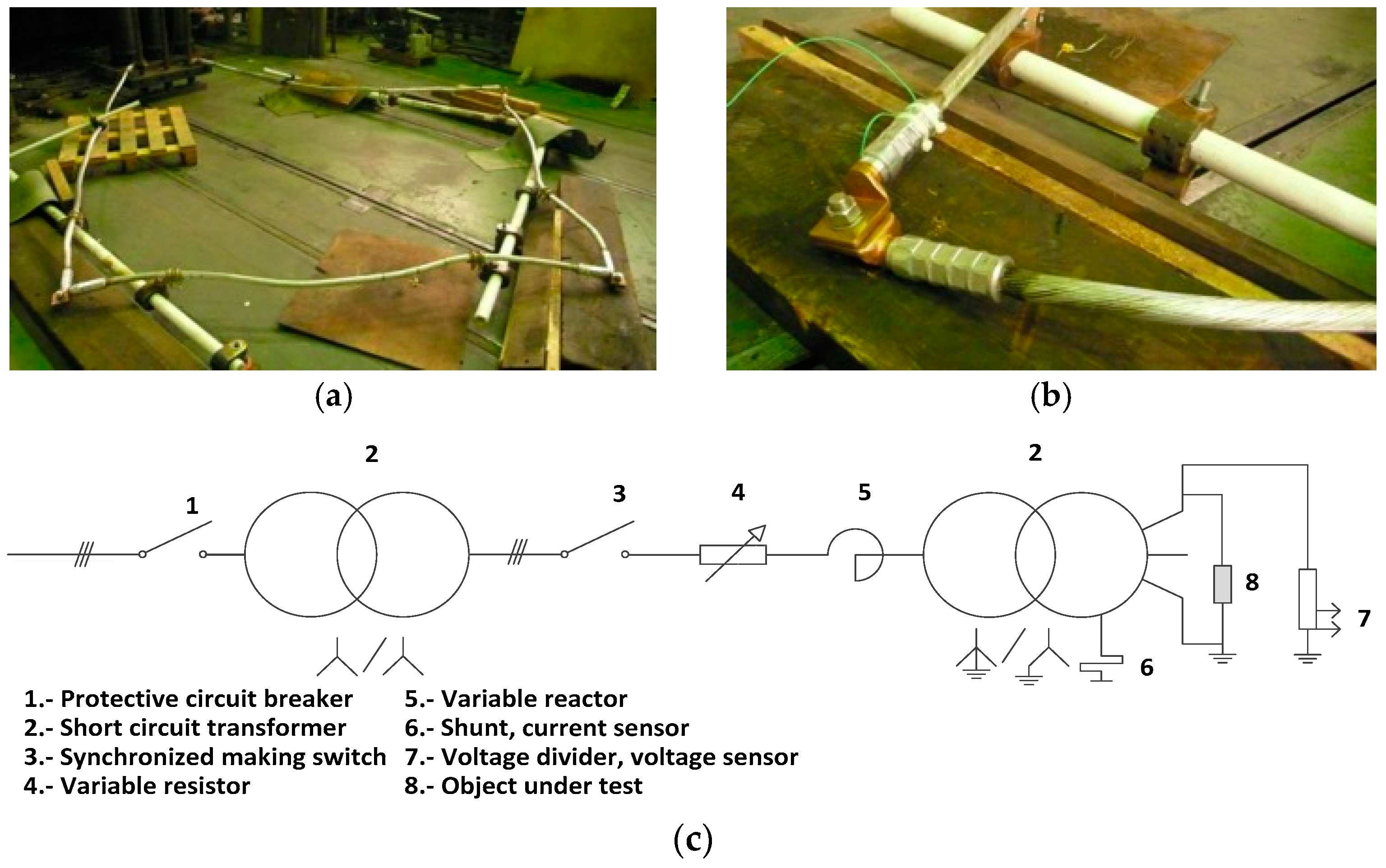
The model proposed in this paper is based on a 3D-FEM model because it is a recognized means to simulate the electromagnetic and thermal behavior of three-dimensional objects with complex shapes [28,29]. The problem under study has to be analyzed by applying a multiphysics approach, since it involves coupled electro-magnetic-thermal physics. To this end, the COMSOL^® Multiphysics package [30] has been used. Joule power losses calculated in the electromagnetic analysis are the heat source used as input data of the thermal analysis, which allows predicting the temperature evolution and distribution in the considered domain.

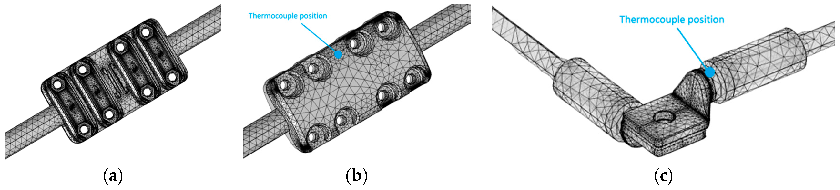
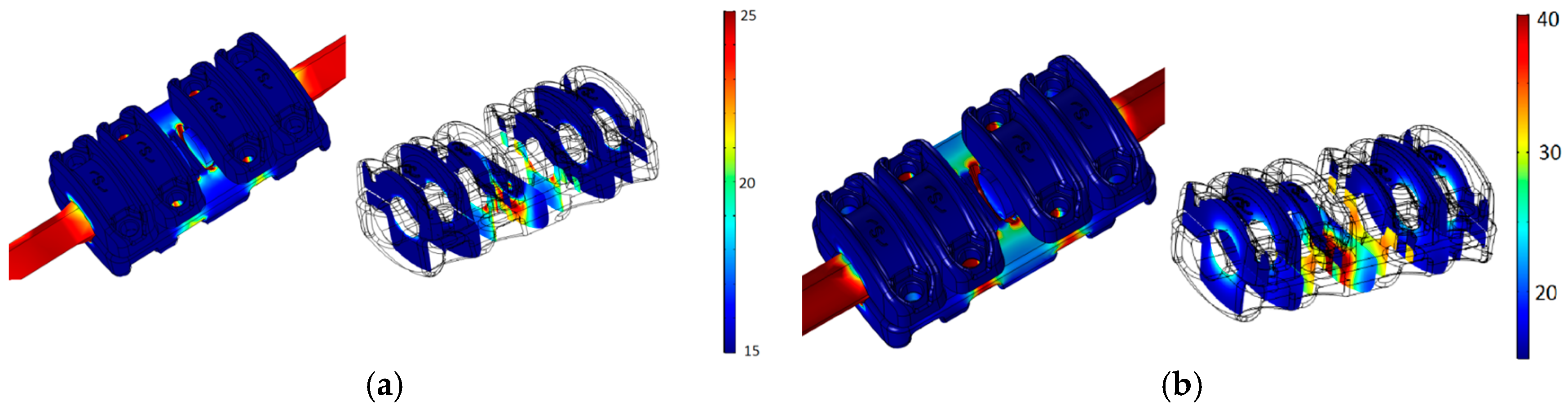
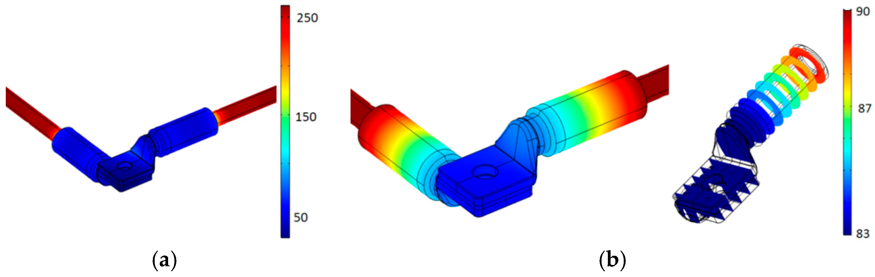
The 3-D mesh applied to the analyzed geometries is composed by 3-D tetrahedra. The mesh of Model A consists of 149,959 domain elements, 34,622 boundary elements, and 8850 edge elements whereas the mesh of Model B consists of 43,016 domain elements, 13,510 boundary elements, and 3426 edge elements.

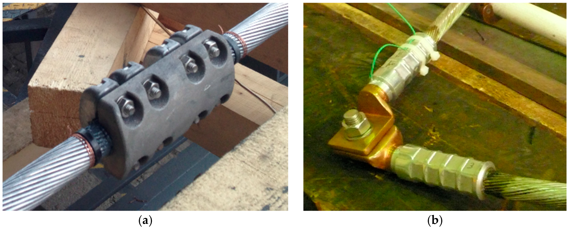
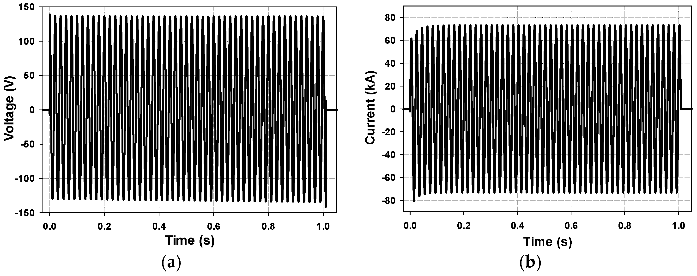
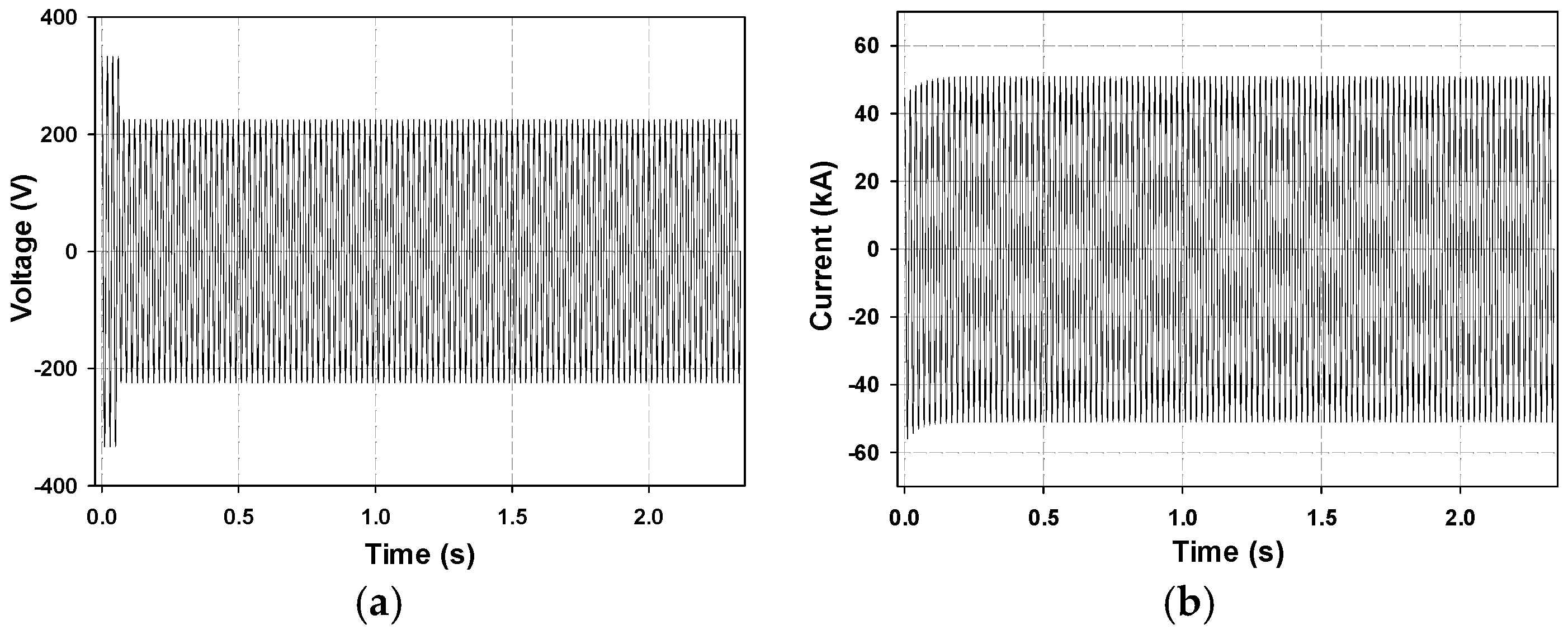
To minimize the thermal influence due to the proximity of the connector, a conductor length of 1.5 m has been modeled in the simulation for both Models A and B.

Figure 3 shows the 3D mesh generated for the two analyzed connectors.

4.1. Electromagnetic Analysis

Since the supply frequency is 50 Hz, the displacement current can be neglected [31] because the quasi-static approximation applies [32], so Maxwell’s equations become:

$$\overrightarrow{\nabla }·\overrightarrow{E}={\mathsf{\rho }}_{\mathrm{e}}/({\mathsf{\epsilon }}_{\mathrm{o}}{\mathsf{\epsilon }}_{\mathrm{r}})$$

(3)

$$\overrightarrow{\nabla }·\overrightarrow{B}=0$$

(4)

$$\overrightarrow{\nabla }\wedge \overrightarrow{E}=-\partial \overrightarrow{B}/\partial t$$

(5)

$$\overrightarrow{\nabla }\wedge \overrightarrow{B}={\mathsf{\mu }}_{\mathrm{o}}{\mathsf{\mu }}_{\mathrm{r}}\overrightarrow{J}$$

(6)

$\overrightarrow{\nabla }·$ and $\overrightarrow{\nabla }\wedge$ are the divergence and rotational operators, respectively; E (V/m) ia the electric field strength; B (T) is the magnetic flux density; J (A/m²) is the electric current density, and ρ_e (C/m³) is the free electric charge density. The charge continuity equation is also considered:

$$\overrightarrow{\nabla }·\overrightarrow{J}=0$$

(7)

The Ohm’s law establishes the relationship between the current density and the electric field as:

$$\overrightarrow{J}={\mathsf{\sigma }}_{\mathrm{e}}\overrightarrow{E}$$

(8)

where σ_e (S/m) is the electrical conductivity.

From Equation (8), the resistive or Joule power losses per unit volume (W/m³) can be calculated as,

$$P_J=\overrightarrow{J}·\overrightarrow{E}$$

(9)

Since the electrical conductivity σ_e is the inverse of the resistivity ρ_e, which depends on temperature [33,34], it can be written as:

$${\mathsf{\sigma }}_{\mathrm{e}}=\frac{1}{{\mathsf{\rho }}_{\mathrm{e},0}[1+{\mathsf{\alpha }}_{\mathrm{e}}(T-T_0)]}$$

(10)

T is the actual temperature; ρ_e,0 is the electrical resistivity measured at T₀ = 293.15 K; and α_e is the temperature coefficient. Therefore, from Equations (8) and (10), Equation (9) results in:

$$P_J=\overrightarrow{J}·\overrightarrow{J}·{\mathsf{\rho }}_{\mathrm{e},0}[1+{\mathsf{\alpha }}_{\mathrm{e}}(T-T_0)]$$

(11)

Resistive losses P_j are the heat source applied in the heat conduction equation detailed below, this being the linkage between the electromagnetic and thermal equations.

Table 2. Electrical and magnetic parameters considered in the model.

Quantity	Symbol	Unit	Value
Free-space permeability	µ0	N/A2	4π × 10−7
Aluminum relative permeability	µr,Al	-	1
A356 alloy relative permeability	µr,A356	-	1
Copper relative permeability	µr,Cu	-	1
Air relative permeability	µr,air	-	1
Free-space permittivity	ε0	F/m	8.85 × 10−12
Aluminum relative permittivity	εr,Al	-	1
A356 alloy relative permittivity	εr,A356	-	1
Copper relative permittivity	εr,Cu	-	1
Air relative permittivity	εr,air	-	1
Aluminum reference resistivity	ρAl	Ω·m	2.77 × 10−8
A356 alloy reference resistivity	ρA356	Ω·m	4.44 × 10−8
Copper reference resistivity	ρCu	Ω·m	1.68 × 10−8
Aluminum temp. coefficient	αAl	1/K	0.0041
A356 alloy temp. coefficient	αA356	1/K	0.0028
Copper temp. coefficient	αCu	1/K	0.0039

summarizes the magnetic and electrical parameters applied in the 3D-FEM model.

Experimental tests carried out with different substation connectors suggest that the contact resistance is approximately twice the resistance of the connector. This value has been considered in this work.

4.2. Thermal Analysis

The well-known three-dimensional heat conduction equation can be expressed as [35]:

$$\mathsf{\rho }{C}_{\mathrm{p}}\frac{\partial T}{\partial t}=-\overrightarrow{\nabla }·\overrightarrow{q}+\overrightarrow{J}·\overrightarrow{E}$$

(12)

ρ (kg/m³) is the volumetric mass density; C_p (J/(kg·K)) is the specific heat capacity; and $\overrightarrow{q}$ (W/m²) is the heat flux density. The term $\overrightarrow{J}·\overrightarrow{E}$ (W/m³) represents the specific power loss due to the Joule effect, that is, the heat source which is expressed as in Equation (11).

The link between the temperature gradient and the heat flux density is provided by the Fourier’s law of heat conduction:

$$\overrightarrow{q}=-k\overrightarrow{\nabla }T$$

(13)

k (W/(m·K)) is the thermal conductivity of the considered material. By combining Equations (11)–(13), the heat conduction equation results in [36]:

$$\mathsf{\rho }{C}_{\mathrm{p}}\frac{\partial T}{\partial t}=k{\nabla }^{2}T+\overrightarrow{J}·\overrightarrow{J}{\mathsf{\rho }}_{\mathrm{e},0}[1+{\mathsf{\alpha }}_{\mathrm{e}}(T-T_0)]$$

(14)

The initial temperature condition for Equation (14) is expressed as:

T(x,y,z,0) = f(x,y,z)

(15)

where f (x,y,z) is the initial (t = 0) temperature distribution in the considered domain.

The natural convection and radiation boundary conditions for Equation (14), can be expressed as [37]:

$$-\overrightarrow{n}(-k\nabla T)=h(T_{\infty }-T)+\mathsf{\epsilon }\mathsf{\sigma }(T_{\infty }^4-T^4)$$

(16)

$\overrightarrow{n}$ is the unit vector normal to the boundary of the analyzed domain; h (W/(m²·K)) is the convection coefficient; T_∞ (K) is the air temperature; T (K) is the surface temperature; ε is the dimensionless emissivity coefficient; and σ (W/(m²·K⁴)) is the Stefan–Boltzmann constant. To calculate the surface-to-ambient radiation, it is assumed that the ambient behaves as a black body at the temperature T_∞.

Table 3. Thermal parameters considered in the model.

Quantity	Symbol	Units	Value
Aluminum mass density	ρAl	kg/m3	2700
A356.0 alloy mass density	ρA356	kg/m3	2685
Copper mass density	ρCu	kg/m3	8700
Aluminum specific heat capacity	Cp,Al	J/(kg·K)	900
A356.0 alloy specific heat capacity	Cp,A356	J/(kg·K)	900
Copper specific heat capacity	Cp,Cu	J/(kg·K)	385
Aluminum thermal conductivity	kAl	W/(m·K)	160
A356 alloy thermal conductivity	kA356	W/(m·K)	151
Copper thermal conductivity	kCu	W/(m·K)	400
Stefan–Boltzmann constant	σ	W/(m2·K4)	5.6704 × 10−8

summarizes the thermal parameters applied in the 3D-FEM model.

4.3. Heat Transfer Coefficients

This paper assumes that the cooling effect contribution is due to the thermal radiation and natural convection, although forced convection is also possible but not applied during the experimental tests. The heat transfer due to convection is often based on coefficients obtained empirically since it is a complex phenomenon and depends upon several variables such as surface dimensions and shape, flow regime, fluid temperature and properties like density, specific heat, thermal conductivity or kinematic viscosity, among others [38,39]. Diverse heat transfer correlations for isothermal surfaces of the most common geometries are found in [40,41]. Since the surfaces of the conductor and connector are not isothermal during the short-circuit evolution, this paper deals with heat transfer coefficients that change with temperature, so during simulations they are reevaluated at each time step.

The Nusselt number of Kuehn and Goldstein [42] has been used for the horizontal cylindrical surfaces of the connectors and the conductors:

$$N{u}_{L\mathrm{c}}=2/\ln (A)$$

(17)

A being calculated as:

$$A=1+\frac{2}{{\left[{\left\{0.518R{a}_{L\mathrm{c}}^{1/4}{\left[1+{(0.559/Pr)}^{3/5}\right]}^{-5/12}\right\}}^{1/15}+{(0.1R{a}_{L\mathrm{c}}^{1/8})}^{1/15}\right]}^{15}}$$

(18)

where Ra_Lc is the dimensionless Rayleigh number, which depends on the characteristic length L_c (m); and Pr is the dimensionless Prandtl number defined below. Note that for the surface of the conductors and the barrels of the connector, L_c is the diameter of the cylinder and, for the surface of the connector, L_c corresponds to the ratio between the surface area and the perimeter.

The Nusselt numbers of McAdams [43] have been applied for the remaining surfaces, since they have been modelled as flat surfaces with downward and upward cooling. According to McAdams, the Nusselt number for downward cooling must be calculated as:

$$N{u}_{L\mathrm{c}}=0.27R{a}_{L\mathrm{c}}^{1/4}{10}^5<R{a}_{L\mathrm{c}}<{10}^{10}$$

(19)

Note that Equation (19) has been used in the connectors’ bottom parts (Model A: the body of the connector; Model B: palm’s surfaces).

The McAdams’ Nusselt number for upward cooling is expressed as:

$$N{u}_{L\mathrm{c}}=0.54R{a}_{L\mathrm{c}}^{1/4}{10}^4<R{a}_{L\mathrm{c}}<{10}^7$$

(20)

which has been applied to the upper parts of the connectors (Model A: caps; Model B: palms’ upper surfaces).

From the dimensionless Nusselt number, the characteristic length L_c (m) and the thermal conductivity k (W/(m·K)), the convective coefficient h can be calculated as [44]:

$$h=\frac{N{u}_{L\mathrm{c}}k}{L_{\mathrm{c}}}$$

(21)

From the dimensionless Prandtl and Grashof numbers, one can calculate the Rayleigh number as:

$$R{a}_{L\mathrm{c}}=G{r}_{L\mathrm{c}}Pr$$

(22)

whereas the dimensionless Prandtl number is obtained as:

$$Pr=C_{\mathrm{p}}\mathsf{\mu }/k$$

(23)

and the Grashof number is:

$$G{r}_{L\mathrm{c}}=\frac{\mathrm{g}\mathsf{\beta }{\mathsf{\rho }}^2{L}_{\mathrm{c}}^3(T_{\mathrm{w}}-T_{\infty })}{{\mathsf{\mu }}^2}$$

(24)

C_p (J/(kg·K)) is the specific heat of air; k (W/(m·K)) is its thermal conductivity, µ (Pa·s) is the dynamic viscosity of air; g (m/s²) is the gravity of earth; β (1/K) is the thermal expansion coefficient, ρ (kg/m³) is the air volumetric mass density, T_w (K) is the surface temperature; and T_∞ (K) is the fluid temperature far from the object’s surface.

Air properties such as µ, ρ and k change with the temperature T_film of the air film, so they are taken from values tabulated in [45] and updated at each time step. T_film is defined as [46]:

$$T_{\text{film}}=\frac{T_{\mathrm{w}}+T_{\infty }}{2}$$

(25)

Emissivity ε in Equation (16) plays a key role in calculating the radiative heat exchange. It is known that emissivity highly depends upon the condition and aging of the radiating surface, although its exact value is often difficult to determine. It is known that, for aluminum conductors, emissivity lies in the range of 0.2–0.9 [47]. Emissivity values considered in this paper are summarized in

Table 4. Emissivity values considered in the model.

Part	Reference	Emissivity
AA-8030 AL conductor	[45]	0.50
AAC conductor	[45]	0.50
Connectors’ surfaces	[48]	0.46

.

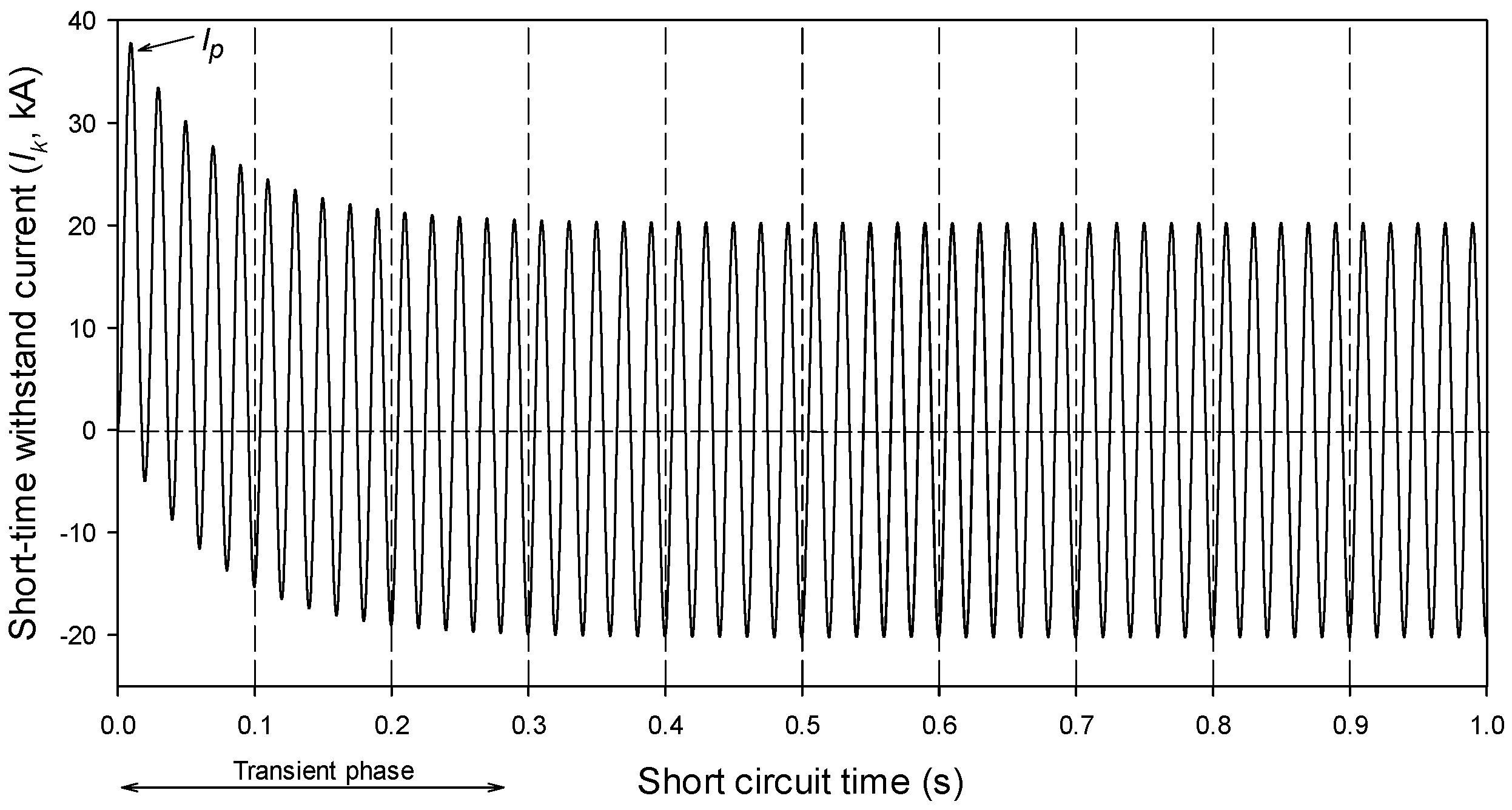
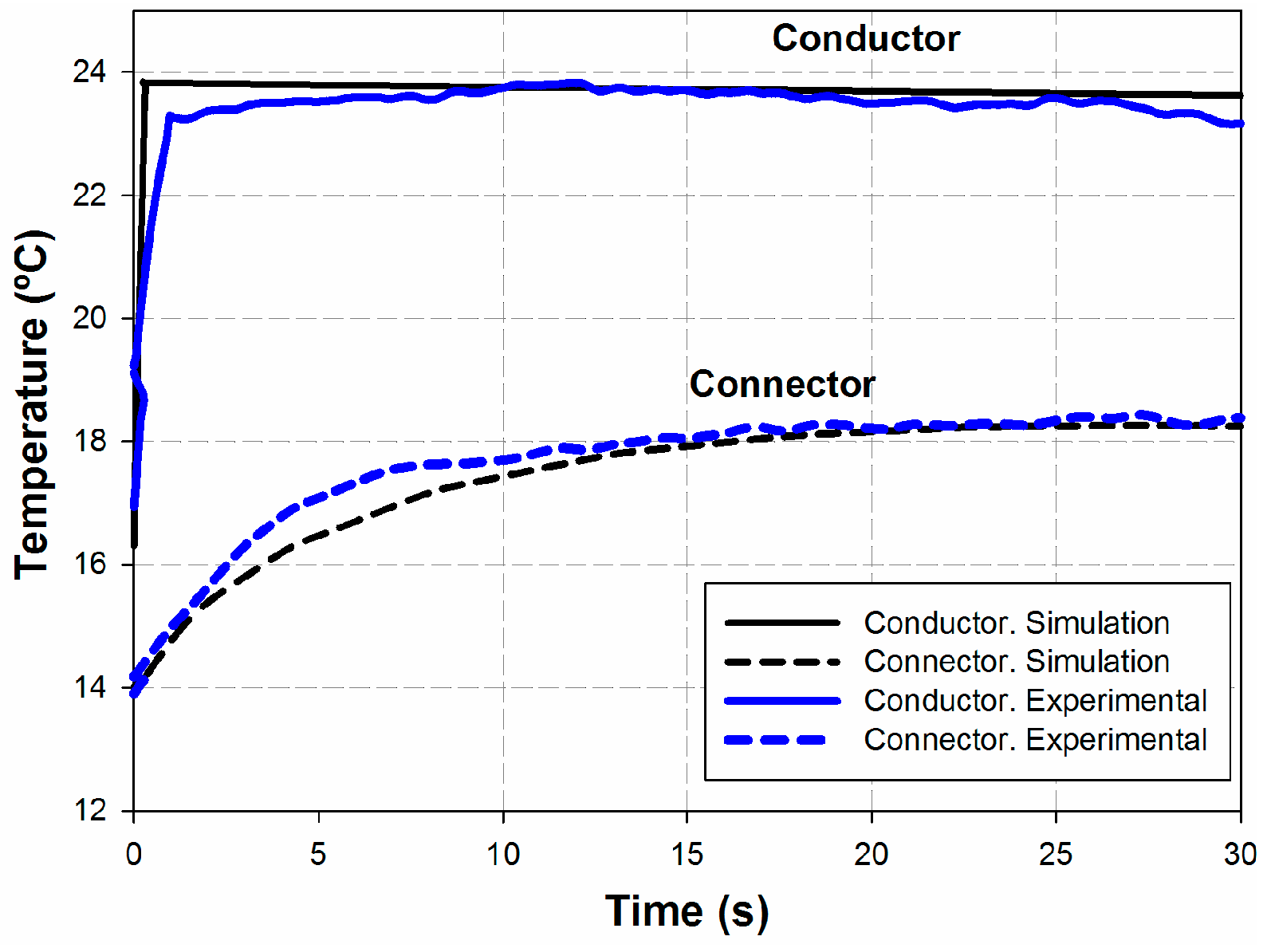
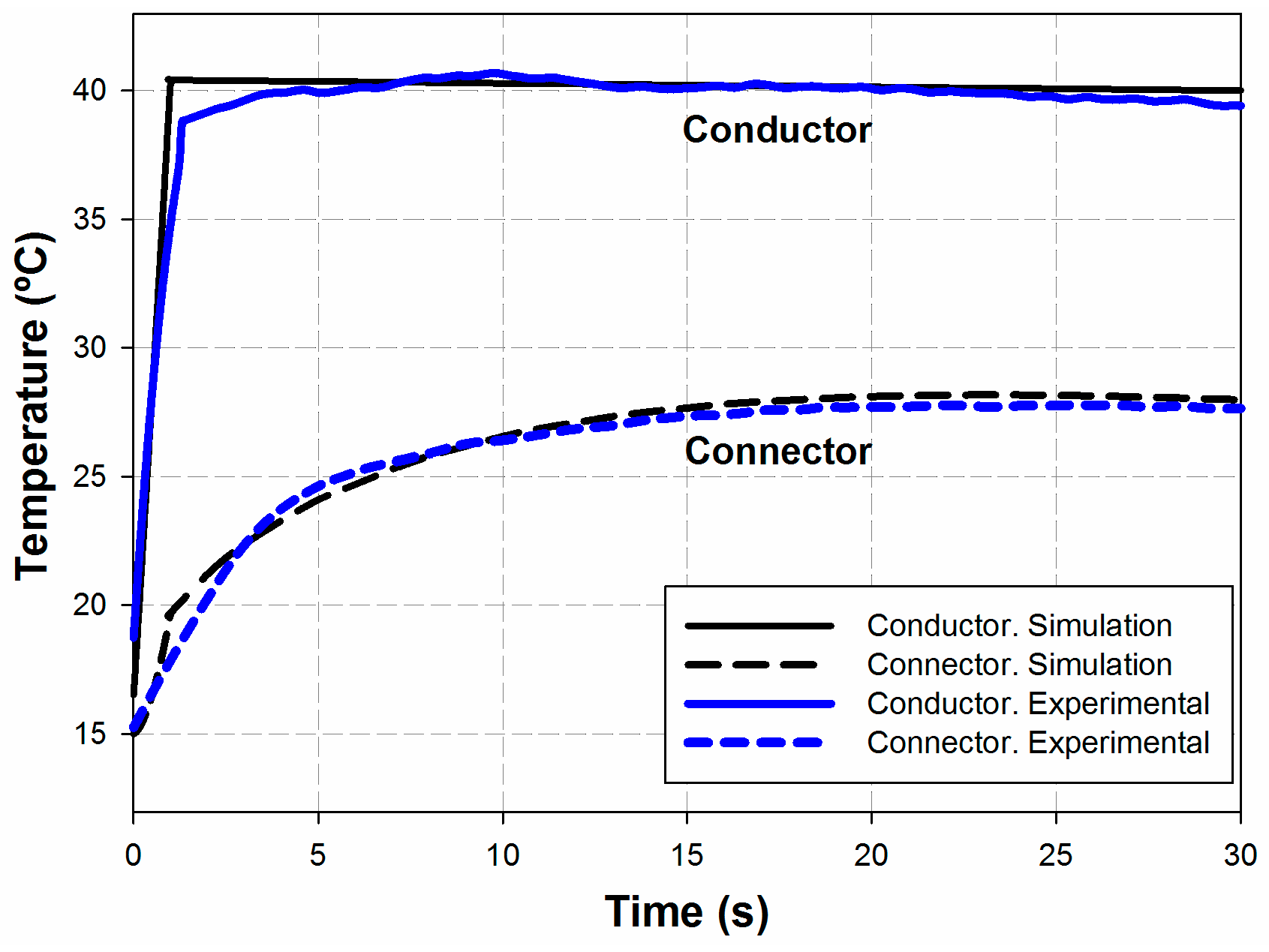
It is noted that cooling contribution due to convection and radiation during the fast short-circuit phase (0.3 s and 1 s for Model A, and 2.275 s for Model B) is very low compared with the power generated by Joule effect. However, the convective and the radiative heat flux have been calculated and taken into account for the entire duration of the test, because convective and radiative phenomena are significant during the cooling phase, that is, once the short-circuit phase has finished.

5. Three-Dimensional Finite Element Method Simulation Results

Simulations were carried out by using as input the experimental current acquired during the short-circuit tests conducted in two laboratories as detailed in Section 6.

5.1. Model A. Simulation of the Short-Time and Peak Withstand Current Tests According to IEC 62271-1:2007 Standard

The prescribed parameters of the short-time and peak withstand current tests are summarized in

Table 5. Prescribed and achieved parameters of the peak withstand current and short-time withstand current tests.

Test	Highest Current (kApeak)		RMS Value of the AC Component (kA)	Joule-Integral (kA2·s)		Test Duration (ms)
	Prescribed	Achieved		Prescribed	Achieved
Peak withstand current	125	126.6	55.1	-	939	307
Short-time withstand current	-	80.55	51.6	2500	2686	1009

.

Figure 4 and Figure 5 show the experimental values of the voltage and current during the peak withstand current test and the short-time withstand current test, respectively. The experimental values of the currents are used as input in the simulations.

Figure 6 shows the temperature distribution at the surfaces of the connector and conductors upon completion of the peak withstand current test and the short-time withstand current test.

5.2. Model B. Simulation of the Short-Circuit Test According to IEC 61238-1:2003 Standard

A second conductor-connector loop intended for low- and medium-voltage systems was tested in order to validate the accuracy and performance of the proposed simulation method. According to the IEC 61238-1:2003 Standard [49] which regulates the short-circuit tests for low- and medium-voltage connectors, the short-circuit current must raise the temperature of the reference conductors from an initial value of 35 °C or below to 250–270 °C. The duration of the short-circuit current shall be in the range [0.9, 1.05] s when applying a maximum current of 25 kA. If the required short-circuit current exceeds this value, a longer duration up to 5 s with a current level between 25 kA and 45 kA can be applied to reach temperatures of 250–270 °C. For the Model B conductor-connector configuration, these requisites are fulfilled under the conditions shown in

Table 6. Values achieved during the short-circuit test conducted according to IEC 61238-1:2003 Standard [49].

Highest Peak Current	Current	Voltage	Joule-Integral	Test Duration
kA	kARMS	VRMS	kA2·s	ms
57.12	36.06	158.89	2960	2275

.

Figure 7 shows the experimental values of the voltage and current during the short-circuit test, which are used as input in the simulations.

Figure 8 shows the temperature distribution at the conductors’ and connector‘s surfaces obtained from FEM simulations.

6. Experimental Versus Simulation Results

6.1. Model A: Experimental Short-Time and Peak Withstand Current Tests According to IEC 62271-1:2007 Standard

To verify the simulation results by means of experimental data, the short-time and peak withstand current tests according to IEC 62271-1:2007 Standard [9] were carried out in Veiki Laboratory (Budapest, Hungary). As shown in Figure 9a, the test loop included two J33SPK couplers and Hawthorn AAC conductors. The tests were carried out at atmospheric conditions (15 °C). The experimental setup includes two three-phase regulating transformers, two three-phase short-circuit transformers, two reactor sets, a protective circuit breaker and a synchronized making switch. The output current and voltage were measured with a calibrated DCM-1 Rogowski coil (uncertainty 0.59%) and a calibrated 1 kV/100 V R-C-R voltage divider (uncertainty 0.26%), respectively, as shown in Figure 9b. Temperature measurements were performed by means of a set of calibrated K-type thermocouples (uncertainty ± 2.2 °C) placed in a small hole of 2 mm depth drilled in the connectors’ bodies and in the central points of each conductor. The thermocouple positions are indicated in Figure 3b. The output signals of the thermocouples were connected to an acquisition card through an analog converter. Temperatures were registered every 100 ms.

Figure 10 shows a comparison between simulation results and the experimental peak withstand current test, until reaching thermal equilibrium. Note that the current shown in Figure 4b is only applied during the first 307 ms, so afterwards there is no current flowing through the tested loop.

Figure 11 shows a comparison between simulation and experimental results of the short-time withstand current test, until reaching thermal equilibrium. The current displayed in Figure 5b is only applied during the first 1009 ms, so later on there is no current flowing through the tested loop.

As shown in Figure 10 and Figure 11, the temperature distribution in the conductors and connectors in both transient and steady state conditions provided by the proposed simulation method shows good agreement with experimental data.

Table 7. Experimental vs. simulation results. Maximum temperature reached during the test for Model A.

Test	Part	Tmeasured (°C)	Tsimulated (°C)	Difference (%)
Peak withstand current test	AAC Conductor	23.9	23.8	0.4%
	J33SPK Connector	18.8	18.3	2.7%
Short-time withstand current test	AAC Conductor	40.7	40.4	0.7%
	J33SPK Connector	27.8	28.1	1.0%

compares the measured and simulated maximum temperatures reached during the tests. Results from Table 7 clearly indicate that differences between experimental and simulation results are always less than 2.7%.

6.2. Model B: Experimental Short-Circuit Test According to IEC 61238-1:2003 Standard

As explained, with the aim to further verify the accuracy of the proposed simulation method, a bimetallic YAT450AM20C terminal for low- and medium-voltage applications was also tested according to the requirements of IEC 61238-1:2003 Standard [49]. The test was conducted in Tecnalia Laboratory (Burtzeña-Barakaldo, Spain). In this case, the test object was a closed loop composed of three pairs of terminal connectors (including M20 bolts composed of A4 CL70 stainless steel) joining 450 mm² AA-8030 AL conductors, as shown in Figure 12. The experimental test was performed indoors at atmospheric conditions (20 °C). The experimental setup consisted of two three-phase short-circuit transformers, a set of variable resistors and reactors, a synchronized making switch and a protective circuit breaker. Output voltage and current were measured, respectively, with a calibrated voltage divider and a calibrated shunt, as shown in Figure 12c. Temperature was recorded by means of an acquisition card connected to a set of thermocouples placed in the connectors’ bodies and the middle points of the conductors.

Measured and simulated maximum temperature values are compared in

Table 8. Experimental vs. FEM simulation results. Maximum temperature reached during the test for Model B.

Part	TMeasured (°C)	TSimulated (°C)	Difference (%)
AA-8030 AL conductor	259.6	258.8	0.3%
YAT450AM20C terminal (barrel)	84.5	85.6	1.3%

. Results from Table 8 show that temperature differences between experimental and simulation results are less than 1.3% for both the conductor and connector. Thus, the experimental results validate the feasibility and accuracy of the proposed simulation method.

Figure 13 compares simulation results and experimental short-circuit test results for both the AA-8030 AL conductor and YAT450AM20C terminal.

7. Conclusions

Substation connectors must pass compulsory short-time withstand current tests and peak withstand current tests, which require very high-power laboratory facilities since they consume huge amounts of electrical power. Such tests are destructive and expensive and the customers frequently have to face long waiting times in performing the tests. Therefore, there is the need to develop specific software tools to simulate such tests in a realistic and economical manner. To this end, this paper has presented an electromagnetic-thermal multiphysics 3D-FEM tool to simulate the transient thermal behavior of substation connectors during standard short-circuit tests. The proposed software tool can also assist in the design process of the connectors while ensuring electromagnetic and thermal requirements imposed by international standards are satisfied, so an optimized design can be achieved. In this way, it is possible to ensure that the optimized substation connectors will pass the compulsory laboratory tests imposed by international standards. Experimental results from standard short-circuit tests conducted in high-current laboratories have proved the suitability and accuracy of the proposed 3D-FEM model.

References

1. Key World Energy Statistics 2015; International Energy Agency: Paris, France, 2015.
2. Li, H.; Bose, A.; Zhang, Y. On-line short-circuit current analysis and preventive control to extend equipment life. IET Gener. Transm. Distrib. 2013, 7, 69–75. [Google Scholar] [CrossRef]
3. Wu, H.; Yuan, L.; Sun, L.; Li, X. Modeling of current-limiting circuit breakers for the calculation of short-circuit current. IEEE Trans. Power Deliv. 2015, 30, 652–656. [Google Scholar] [CrossRef]
4. Tartaglia, M.; Mitolo, M. An analytical evaluation of the prospective to assess short-circuit capabilities of cables and busways. IEEE Trans. Power Deliv. 2010, 25, 1334–1339. [Google Scholar] [CrossRef]
5. Palani, A.; Santhi, S.; Gopalakrishna, S.; Jayashankar, V. Real-time techniques to measure winding displacement in transformers during short-circuit tests. IEEE Trans. Power Deliv. 2008, 23, 726–732. [Google Scholar] [CrossRef]
6. Schlabbach, J.; Rofalski, K.H. Power System Engineering: Planning, Design, and Operation of Power Systems and Equipment; Wiley-VCH Verlag GmbH & Co. KGaA: Weinheim, Germany, 2008. [Google Scholar]
7. Capelli, F.; Riba, J.-R.; Gonzalez, D. Optimization of Short-Circuit Tests Based on Finite Element Analysis. In Proceedings of the 2015 IEEE International Conference on Industrial Technology (ICIT), Seville, Spain, 17–19 March 2015; pp. 1368–1374.
8. Common Specifications for High-Voltage Switchgear and Controlgear Standards; IEC 60694; International Electrotechnical Commission: London, UK, 1996.
9. High-Voltage Switchgear and Controlgear—Part 1: Common Specifications; IEC 62271-1:2007; International Electrotechnical Commission: London, UK, 2007.
10. Switchgear-Metal-Enclosed Low-Voltage AC Power Circuit Breaker Switchgear Assemblies-Conformance Test Procedures; ANSI C37.51a-2010; American National Standards Institute: Washington, DC, USA, 2011.
11. Qu, J.; Wang, Q.; Zhang, J.; Zhao, H.; Wu, G.; Li, X. 3-D transient finite-element analysis and experimental investigation of short-circuit dynamic stability for air circuit breaker. IEEE Trans. Compon. Packag. Manuf. Technol. 2015, 5, 1610–1617. [Google Scholar]
12. Guan, X.; Shu, N.; Kang, B.; Zou, M. Multiphysics analysis of plug-in connector under steady and short circuit conditions. IEEE Trans. Compon. Packag. Manuf. Technol. 2015, 5, 320–327. [Google Scholar] [CrossRef]
13. Wilkins, R.; Saengsuwan, T.; O’Shields, L. Short-circuit tests on current-limiting fuses: Modelling of the test circuit. IEE Proc. C Gener. Transm. Distrib. 1993, 140, 30–36. [Google Scholar] [CrossRef]
14. Hernández-Guiteras, J.; Riba, J.-R.; Romeral, L. Improved design of an extra-high-voltage expansion substation connector through magnetic field analysis. Simul. Model. Pract. Theory 2014, 43, 96–105. [Google Scholar] [CrossRef]
15. Takahashi, T.; Ito, T.; Okamoto, T.; Imajo, T. Development of Calculation System for Transient Temperature Rise of Power Cables in Protection Pipe. In Proceedings of the IEEE/PES Transmission and Distribution Conference and Exhibition 2002: Asia Pacific, Yokohama, Japan, 6–10 October 2002; Volume 3, pp. 1899–1904.
16. Li, Y.Y.; Liang, Y.; Li, Y.Y.; Si, W.; Yuan, P.; Li, J. Coupled Electromagnetic-Thermal Modeling the Temperature Distribution of XLPE Cable. In Proceedings of the 2009 Asia-Pacific Power and Energy Engineering Conference, Wuhan, China, 27–31 March 2009; pp. 1–4.
17. Yoon, J.-H.; Ahn, H.-S.; Choi, J.; Oh, I.S. An Estimation Technology of Temperature Rise in GIS Bus Bar using Three-Dimensional Coupled-Field Multiphysics. In Proceedings of the Conference Record of the 2008 IEEE International Symposium on Electrical Insulation, Vancouver, BC, Canada, 9–12 June 2008; pp. 432–436.
18. Hameyer, K.; Driesen, J.; De Gersem, H.; Belmans, R. The classification of coupled field problems. IEEE Trans. Magn. 1999, 35, 1618–1621. [Google Scholar] [CrossRef]
19. Buonanno, G. Effect of radiative and convective heat transfer on thermal transients in power cables. IEE Proc. Gener. Transm. Distrib. 1995, 142, 436–444. [Google Scholar] [CrossRef]
20. Kim, S.W.; Kim, H.H.; Hahn, S.C.; Lee, B.Y.; Park, K.Y.; Shin, Y.J.; Song, W.P.; Kim, J.B.; Shin, I.H. Coupled finite-element-analytic technique for prediction of temperature rise in power apparatus. IEEE Trans. Magn. 2002, 38, 921–924. [Google Scholar] [CrossRef]
21. Spaeck-Leigsnering, Y.; Gjonaj, E.; De Gersem, H.; Weiland, T.; Giebel, M.; Hinrichsen, V. Electro-quasistatic-thermal modeling and simulation of station class surge arresters. IEEE Trans. Magn. 2015, 52. [Google Scholar] [CrossRef]
22. Liao, C.; Ruan, J.; Liu, C.; Wen, W.; Du, Z. 3-D coupled electromagnetic-fluid-thermal analysis of oil-immersed triangular wound core transformer. IEEE Trans. Magn. 2014, 50. [Google Scholar] [CrossRef]
23. Arroyo, A.; Castro, P.; Martinez, R.; Manana, M.; Madrazo, A.; Lecuna, R.; Gonzalez, A. Comparison between IEEE and CIGRE thermal behaviour standards and measured temperature on a 132-kV overhead power line. Energies 2015, 8, 13660–13671. [Google Scholar] [CrossRef]
24. Li, X.; Qu, J.; Wang, Q.; Zhao, H.; Chen, D. Numerical and experimental study of the short-time withstand current capability for air circuit breaker. IEEE Trans. Power Deliv. 2013, 28, 2610–2615. [Google Scholar] [CrossRef]
25. C37.20.1-2015—IEEE Standard for Metal-Enclosed Low-Voltage (1000 Vac and below, 3200 Vdc and below) Power Circuit Breaker Switchgear; IEEE Standard Department: Piscataway, NJ, USA, 2015; pp. 1–84.
26. C37.13.1-2006—IEEE Standard for Definite-Purpose Switching Devices for Use in Metal-Enclosed Low-Voltage Power Circuit Breaker Switchgear; IEEE Standard Department: Piscataway, NJ, USA, 2006.
27. Geng, Y.; Yan, J.; Liu, Z.; Yao, J. Development of a 126 kV Single-Break Vacuum Circuit Breaker and Type Test. In Proceedings of the 2013 2nd International Conference on Electric Power Equipment—Switching Technology (ICEPE-ST), Matsue, Japan, 20–23 October 2013; pp. 1–4.
28. Holyk, C.; Liess, H.-D.; Grondel, S.; Kanbach, H.; Loos, F. Simulation and measurement of the steady-state temperature in multi-core cables. Electr. Power Syst. Res. 2014, 116, 54–66. [Google Scholar] [CrossRef]
29. Soulinaris, G.K.; Halevidis, C.D.; Polykrati, A.D.; Bourkas, P.D. Evaluation of the thermal stresses and dielectric phenomena in the investigation of the causes of wildfires involving distribution power lines. Electr. Power Syst. Res. 2014, 117, 76–83. [Google Scholar] [CrossRef]
30. Comsol COMSOL 4.3 Multiphysics User’s Guide 2012; COMSOL: Stockholm, Sweden, 2012.
31. Riba, J.-R. Analysis of formulas to calculate the AC resistance of different conductors’ configurations. Electr. Power Syst. Res. 2015, 127, 93–100. [Google Scholar] [CrossRef] [Green Version]
32. Maxwell, J.C.; Torrance, T.F. A Dynamical Theory of the Electromagnetic Field; Wipf and Stock Publishers: Eugene, OR, USA, 1996. [Google Scholar]
33. Kasap, S.O. Principles of Electronic Materials and Devices; McGraw-Hill: New York, NY, USA, 2006. [Google Scholar]
34. Electric Cables—Calculation of the Current Rating—Part 1-1: Current Rating Equations (100% Load Factor) and Calculation of Losses—General; IEC 60287-1-1:2006; International Electrotechnical Commission: Geneva, Switzerland, 2006.
35. Özişik, M.N. Heat Transfer: A Basic Approach; McGraw-Hill: New York, NY, USA, 1985. [Google Scholar]
36. Acevedo, L.; Usón, S.; Uche, J. Numerical study of cullet glass subjected to microwave heating and SiC susceptor effects. Part I: Combined electric and thermal model. Energy Convers. Manag. 2015, 97, 439–457. [Google Scholar] [CrossRef]
37. Fernandez, E.; Torres, E.; Zamora, I.; Mazon, A.J.; Albizu, I. Thermal model for current limiting fuses installed in vertical position. Electr. Power Syst. Res. 2014, 107, 167–174. [Google Scholar] [CrossRef]
38. Kakaç, S.; Yener, Y. Convective Heat Transfer, 2nd ed.; CRC Press: Boca Raton, Fl, USA, 1994. [Google Scholar]
39. Yu, B.; Zhang, S.; Yan, J.; Cheng, L.; Zheng, P. Thermal analysis of a novel cylindrical transverse-flux permanent-magnet linear machine. Energies 2015, 8, 7874–7896. [Google Scholar] [CrossRef]
40. Lienhard, J.H. A Heat Transfer Textbook: Fourth Edition; Courier Corporation: North Chelmsford, MA, USA, 2013. [Google Scholar]
41. Bejan, A. Convection Heat Transfer; John Wiley & Sons: New York, NY, USA, 2013. [Google Scholar]
42. Kuehn, T.H.; Goldstein, R.J. Correlating equations for natural convection heat transfer between horizontal circular cylinders. Int. J. Heat Mass Transf. 1976, 19, 1127–1134. [Google Scholar] [CrossRef]
43. McAdams, W.H. Heat Transmission; McGraw-Hill Inc.: New York, NY, USA, 1954. [Google Scholar]
44. Yang, F.; Ran, W.; Chen, T.; Luo, X. Investigation on the factors affecting the temperature in urban distribution substations and an energy-saving cooling strategy. Energies 2011, 4, 314–323. [Google Scholar] [CrossRef]
45. IEEE Standard for Calculating the Current-Temperature of Bare Overhead Conductors; IEEE Standard Department: Piscataway, NJ, USA, 2007.
46. Zhao, J.; Cheng, C.; Song, Y.; Liu, W.; Liu, Y.; Xue, K.; Zhu, Z.; Yang, Z.; Wang, D.; Yang, M. Heat transfer analysis of methane hydrate sediment dissociation in a closed reactor by a thermal method. Energies 2012, 5, 1292–1308. [Google Scholar] [CrossRef]
47. Taylor, C.S.; House, H.E. Emissivity and its effect on the current-carrying capacity of stranded aluminum conductors [includes discussion]. Trans. Am. Inst. Electr. Eng. Part III Power Appar. Syst. 1956, 75. [Google Scholar] [CrossRef]
48. Öhman, C. Emittansmätningar med AGEMA E-Box; AGEMA: Stockholm, Sweden, 1999. [Google Scholar]
49. Compression and Mechanical Connectors for Power Cables for Rated Voltages up to 30 kV (Um = 36 kV)—Part 1: Test Methods and Requirements; IEC 61238-1:2003; International Electrotechnical Commission: Geneva, Switzerland, 2003.
Figure 1. Short-time withstand current (Ik) and peak withstand current (Ip).
Energies 09 00418 g001
Figure 2. (a) Two-cap J33SPK coupler substation connector; and (b) bimetallic YAT450AM20C T connector.
Energies 09 00418 g002
Figure 3. (a) Model A. Mesh of the top-side of the two-cap J33SPK coupler substation connector; (b) bottom-side; and (c) Model B used to validate the three-dimensional finite element method (3D-FEM) model proposed in this paper. Mesh of the YAT450AM20C bimetallic compression connector.
Energies 09 00418 g003
Figure 4. Experimental (a) voltage and (b) current values during the peak withstand current test.
Energies 09 00418 g004
Figure 5. Experimental (a) voltage and (b) current values during the short-time withstand current test.
Energies 09 00418 g005
Figure 6. Model A. (a) Simulated temperature distribution (°C) upon completion of the peak withstand current test (t = 0.3 s) according to IEC 62271-1:2007 Standard [9]. (b) Simulated temperature distribution (°C) upon completion of the short-time withstand current test (t = 1 s) according to IEC 62271-1:2007 Standard [9].
Energies 09 00418 g006
Figure 7. Test (a) voltage and (b) current measured during the short-circuit test.
Energies 09 00418 g007
Figure 8. Model B. (a) Simulated temperature distribution (°C) upon completion of the short-circuit test (t = 2.275 s) according to IEC 61238-1:2003 Standard [49]. Conductors and YAT450AM20C bimetallic compression connector; (b) Simulated temperature distribution (°C) of the YAT450AM20C bimetallic compression connector at equilibrium temperature (t = 450 s).
Energies 09 00418 g008
Figure 9. (a) Tested loop; (b) test circuit to perform the short-time withstand current test and peak withstand current test.
Energies 09 00418 g009
Figure 10. Experimental vs. 3D-FEM simulation results. Temperature evolution during the peak withstand current test until reaching the equilibrium temperature. Bottom part of the J33SPK coupler substation connector (connector’s body) and AAC conductor.
Energies 09 00418 g010
Figure 11. Experimental vs. 3D-FEM simulation results. Temperature evolution during the short-time withstand current test until reaching thermal equilibrium. Bottom part of J33SPK coupler substation connector (connector’s body) and AAC conductor.
Energies 09 00418 g011
Figure 12. (a) Experimental setup: tested loop composed of an AA-8030 AL conductor and class-A YAT450AM20C terminals; (b) bimetallic YAT450AM20C terminals: thermocouples are placed at the barrel's surface; and (c) test circuit to perform the short-circuit test.
Energies 09 00418 g012
Figure 13. Experimental vs. 3D-FEM simulation results. Temperature evolution during the short-circuit test according to IEC 61238-1 Standard [49] and until reaching thermal equilibrium.
Energies 09 00418 g013