Development of Near Optimal Rule-Based Control for Plug-In Hybrid Electric Vehicles Taking into Account Drivetrain Component Losses

Abstract

A near-optimal rule-based mode control (RBC) strategy was proposed for a target plug-in hybrid electric vehicle (PHEV) taking into account the drivetrain losses. Individual loss models were developed for drivetrain components including the gears, planetary gear (PG), bearings, and oil pump, based on experimental data and mathematical governing equations. Also, a loss model for the power electronic system was constructed, including loss from the motor-generator while rotating in the unloaded state. To evaluate the effect of the drivetrain losses on the operating mode control strategy, backward simulations were performed using dynamic programming (DP). DP selects the operating mode, which provides the highest efficiency for given driving conditions. It was found that the operating mode selection changes when drivetrain losses are included, depending on driving conditions. An operating mode schedule was developed with respect to the wheel power and vehicle speed, and based on the operating mode schedule, a RBC was obtained, which can be implemented in an on-line application. To evaluate the performance of the RBC, a forward simulator was constructed for the target PHEV. The simulation results show near-optimal performance of the RBC compared with dynamic-programming-based mode control in terms of the mode operation time and fuel economy. The RBC developed with drivetrain losses taken into account showed a 4%–5% improvement of the fuel economy over a similar RBC, which neglected the drivetrain losses.

1. Introduction

Plug-in hybrid electric vehicles (PHEV) have relatively large battery capacities and can drive on electric power (enough for most daily commutes), and the range can be considerably extended with an internal combustion engine (ICE). As a result, PHEVs are considered to be a highly competitive solution to meet the ever-strengthening regulations of CO₂ emissions and fuel consumption [1]. When a PHEV is operated using the ICE and electric motor in combination, the overall efficiency depends on how the power is distributed between the ICE and motor, which is determined by the system configuration and its control strategy [2].

To improve efficiency, various configurations of the ICE, motor and generator (MG) have been investigated [3]. In general, PHEVs utilize more than one operating mode to provide the demanded performance, where the selected mode is determined by the instantaneous system efficiency and the battery state of charge (SOC). Since PHEV efficiency depends on the power transmission characteristics, which vary with the operating mode [4,5,6], developing an optimized operating mode control strategy is essential.

Several studies have been carried out investigating various operating mode control strategies. Most control strategies use rule-based control to provide demanded power for given driving conditions using heuristic-based data, or equivalent fuel consumption minimization methods [7,8,9,10]. The mode control algorithm selects the operating mode which provides the highest system efficiency for given driving conditions [11]. The mode control algorithm considers only instantaneous driving conditions rather than the whole future driving cycle, so it can only guarantee local optimality. For optimization of the on-line application, rule-based control was developed using post-processed DP results [12,13], and using the Pontryagin’s minimum principle, which reduces the computation time to implement in the controller [14,15,16,17,18]. In addition, fuel economy improvement strategy was proposed using a neural network-based fuel consumption computational model [19]. However, most of these studies only considered the efficiency of the ICE and MGs in the construction of rule-based controls, dynamic programming (DP), and Pontryagin’s minimum principle [20,21,22], except for a few works which include the final reduction gear loss as a constant [23].

In PHEVs, power from the ICE and MGs is transmitted along the drivetrain components, including gears, planetary gears (PGs), clutch, brakes, bearings, etc. Whenever power flows through drivetrain components, losses occur, which vary depending on torque and speed. In addition, when the operating mode is changed, the power path changes and the number of drivetrain components in which the power flows changes. Therefore, neglecting drivetrain component losses in designing our control strategy could adversely impact system efficiency.

In this study, a near-optimal rule-based mode control (RBC) strategy is proposed for a target PHEV, taking into account the drivetrain component losses. Loss models are developed based on experimental data and governing equations. The effects of the component losses on the PHEV system efficiency are investigated using DP. Based on these results, a near-optimal control strategy is proposed and its performance is evaluated.

2. System Description

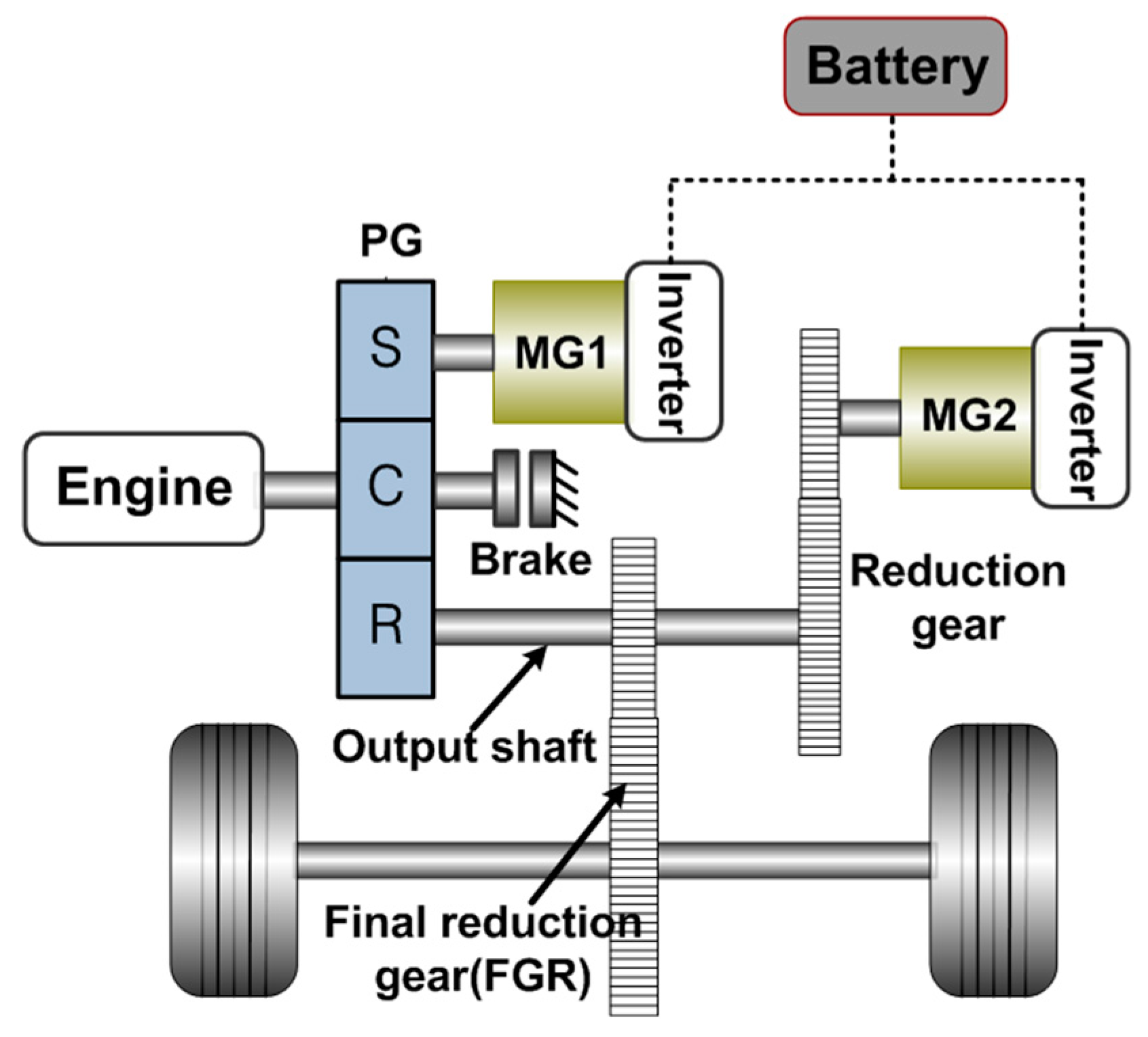
In Figure 1, a schematic diagram of the target PHEV is shown. The system is comprised of one PG, two reduction gears, two MGs (MG1 and MG2), and one brake. The engine is connected to the carrier, MG1 is connected to the sun gear of the PG, and MG2 is connected to the output shaft through the reduction gear. Since the target PHEV system is a power-split type, power is transmitted through mechanical and electrical paths. Using MG1 and PG, the engine speed can be controlled continuously, independent of the vehicle speed. The PHEV in Figure 1 is basically the same as a Toyota Prius, except for the brake. When engaging the brake, electric driving mode “EV#2” is implemented using MG1 and MG2 in combination, which is not seen in the Prius. This configuration is called “Prius+” [24].

The target PHEV utilizes three operating modes: (1) EV#1; (2) EV#2; and (3) power split (PS), as shown in

Table 1. Operating modes for target PHEV system. PS: power split.

Operating Mode	Brake	MG1	MG2	Engine
EV#1	Disengaged	Off	On	Off
EV#2	Engaged	On	On	Off
PS	Disengaged	On	On	On

. EV#1 and PS modes are implemented without application of the brake, as in the Prius Toyota hybrid system (THS). EV#2 mode is activated by engaging the brake.

2.1. Speed and Torque Analysis for Target Plug-In Hybrid Electric Vehicle

The relationship between speed and torque of MG1, MG2, engine, and wheels was obtained for each driving mode using lever analysis [24,25].

2.1.1. EV#1 Mode

The vehicle is propelled by MG2. The wheel torque is supplied by MG2. The speed of MG2 is proportional to the vehicle speed by the reduction gear ratio.

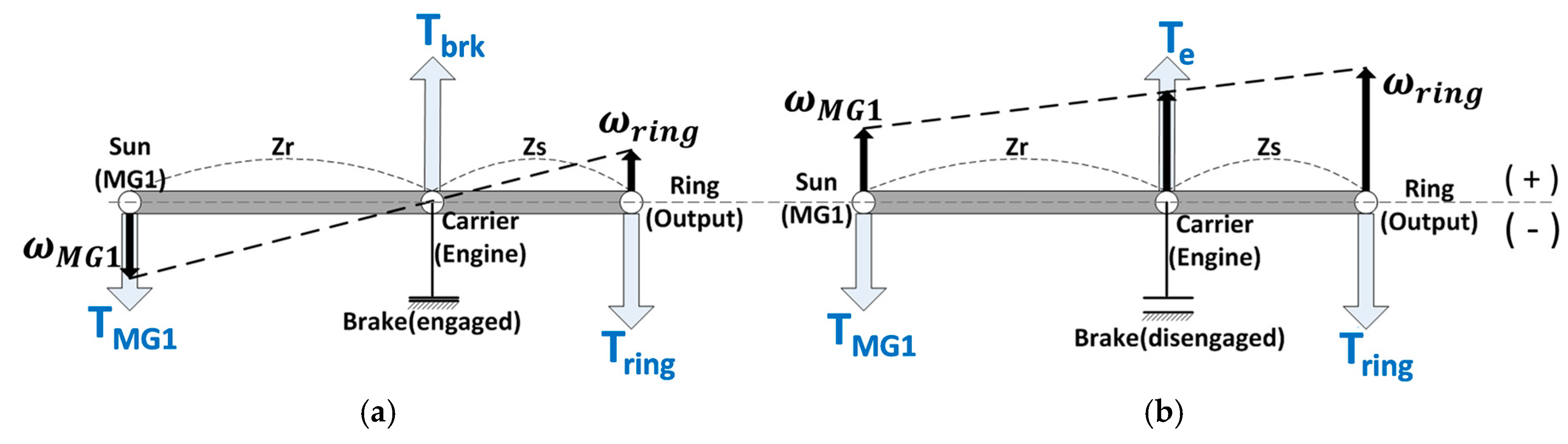
2.1.2. EV#2 Mode

The brake is engaged, so the engine does not work. The vehicle is propelled by MG2 and MG1. According to the lever analysis in Figure 2a, the speed and torque equation can be represented as:

$$\left[\begin{array}{c}{\mathsf{\omega }}_{\text{MG}1}\\ {\mathsf{\omega }}_{\text{MG}2}\end{array}\right]=\left[\begin{array}{cc}{N}_{\text{FGR}}{N}_{\text{PG}}& 0\\ N_{\text{FGR}}{N}_{\text{RG}}& 0\end{array}\right]\left[\begin{array}{c}{\mathsf{\omega }}_{\text{whl}}\\ {\mathsf{\omega }}_{\mathrm{e}}\end{array}\right]$$

(1)

$$\left[T_{\text{whl}}\right]=\left[\begin{array}{cc}{N}_{\text{RG}}{N}_{\text{FGR}}& N_{\text{PG}}{N}_{\text{FGR}}\end{array}\right]\left[\begin{array}{c}{T}_{\text{MG}2}\\ T_{\text{MG}1}\end{array}\right]$$

(2)

where T is the torque, and ω is the speed. The subscripts MG1, MG2, FGR, PG, RG, whl, and e represent MG1, MG2, final reduction gear ratio, PG, reduction gear, wheel, and engine, respectively.

Figure 2a shows that the MG1 power is positive in the EV#2 mode since the torque and speed are both negative, which implies that MG1 acts as a driving motor. In this mode, vehicle efficiency is determined by the torque distribution ratio between MG1 and MG2.

2.1.3. Power Split Mode

In PS mode, the brake is disengaged and the speed and torque of the MGs are determined by the engine and wheels. Since the engine is controlled by MG1 to operate on the optimal operation line (OOL) [26], the speed and torque of MG1 and MG2 can be calculated from the speed and torque of the engine on the OOL and wheel speed and torque using the speed and torque lever (Figure 2) as follows:

$$\left[\begin{array}{c}{\mathsf{\omega }}_{\text{MG}1}\\ {\mathsf{\omega }}_{\text{MG}2}\end{array}\right]=\frac{1}{Z_{\mathrm{s}}}\left[\begin{array}{cc}-Z_{\mathrm{r}}& Z_{\mathrm{s}}+Z_{\mathrm{r}}\\ N_{\text{FGR}}\times Z_{\mathrm{r}}& 0\end{array}\right]\left[\begin{array}{c}{\mathsf{\omega }}_{\text{whl}}\\ {\mathsf{\omega }}_{\mathrm{e}}\end{array}\right]$$

(3)

$$\left[\begin{array}{c}{T}_{\text{MG}1}\\ T_{\text{MG}2}\end{array}\right]=\left[\begin{array}{cc}0& -\frac{Z_s}{Z_{\mathrm{s}}+Z_{\mathrm{r}}}\\ \frac{1}{N_{\text{RG}}{N}_{\text{FGR}}}& -\frac{Z_{\mathrm{r}}}{Z_{\mathrm{s}}+Z_{\mathrm{r}}}\end{array}\right]\left[\begin{array}{c}{T}_{\text{whl}}\\ T_{\mathrm{e}}\end{array}\right]$$

(4)

where Z is the gear teeth number, and the subscripts s and r represent the sun gear and ring gear, respectively.

As shown in Figure 2b, the power of MG1 is negative in PS mode because its speed is positive and torque is negative. MG1 acts as a power conversion device in this mode, transforming mechanical power into electrical power.

3. Component Loss Model

In the target PHEV, power losses occur in the drivetrain components and the power electronics system. In this study, loss models of each component are developed.

3.1. Drivetrain Component Losses

3.1.1. Gear Loss

To calculate the gear loss, Coulomb’s law of friction has been applied, which is a function of the tooth normal force, the coefficient of friction, and the sliding speed at each contact point [27]. In this study, gear torque loss was assumed to be 1% of the transmitted torque [23], which is a widely used general rule in the automotive industry.

3.1.2. Planetary Gear Loss

The PG consists of the sun, pinion, and ring gears. PG loss occurs mostly due to friction when the gear teeth are meshing. PG torque loss is represented by considering the meshing condition as follows [28,29]:

$$T_{\text{loss}\_\text{PG}}=\{\begin{array}{ll}{C}_{\text{PG}}\times T_{\text{in}\_\text{PG}},& \text{when carrier is fixed}\\ C_{\text{PG}}\times \left(\frac{Z_{\mathrm{r}}}{Z_{\mathrm{r}}+Z_{\mathrm{s}}}\right)\times T_{\text{in}\_\text{PG}}& \text{when ring gear is fixed}\\ C_{\text{PG}}\times \left(\frac{Z_{\mathrm{s}}}{Z_{\mathrm{r}}+Z_{\mathrm{s}}}\right)\times T_{\text{in}\_\text{PG}}& \text{when sun gear is fixed}\end{array}$$

(5)

where $T_{\text{loss}}$ is the torque loss, $T_{\text{in}}$ is the input torque, C is the coefficient of friction. The subscript _PG indicates the PG.

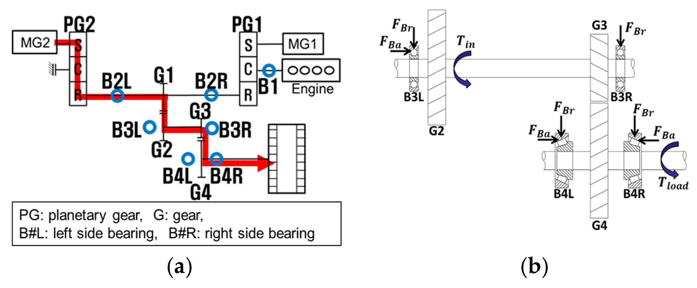
3.1.3. Bearing Loss

Bearing loss consists of loaded and unloaded losses. Loaded loss is due to the bearing load, while unloaded loss occurs due to friction between the rotating surface and the lubrication oil film. In the target PHEV, the bearing load depends on the operating mode. In Figure 3a, the bearings in the target PHEV and the power flow are shown in EV#1 mode. In EV#1 mode, bearings B2L, B2R, B3L, B3R, B4L, and B4R are loaded, while bearing B1 is unloaded and free-rotating. In this study, taper roller bearings were used for B4L and B4R, and deep-grooved ball bearings for the other bearings. The load at each bearing can be calculated using the moment and force equilibrium equations from the free body diagram in Figure 3b.

The bearing load in EV#2 and PS modes can be obtained in a similar manner. Once the bearing load is determined, the loaded loss is calculated as follows [27,30]:

$${P_1}^a=3F_{\text{Ba}}-0.1F_{\text{Br}}$$

(6)

$$T_{\text{loss}\_\text{BRGload}}=f_1\times {P_1}^a\times {d_{\mathrm{m}}}^b\times {10}^{-3}$$

(7)

where a, b, and f₁ are coefficients for bearing type, P₁ is the equivalent bearing load, F_Ba is the axial bearing reaction force, F_Br is the radial bearing reaction force, and d_m is the bearing mean diameter.

Bearing unloaded loss occurs due to the slip between the rotating surface and lubrication oil film, which is represented as a function of the kinematic viscosity and rotational speed:

$$T_{\text{loss}\_\text{BRGunload}}=\{\begin{array}{c}1.6\times {10}^{-8}\times f_0\times {d_{\mathrm{m}}}^3, if \left({\upsilon }_{\text{oil}}\times n\right)<\frac{2000{\text{mm}}^2}{\mathrm{s}\cdot \text{min}}\\ {10}^{-10}\times f_0\times {\left({\upsilon }_{\text{oil}}\times n\right)}^{\frac{2}{3}}\times {d_{\mathrm{m}}}^3, if \left({\upsilon }_{\text{oil}}\times n\right)\ge \frac{2000{\text{mm}}^2}{\mathrm{s}\cdot \text{min}}\end{array}$$

(8)

where f₀ is the coefficient for bearing unloaded loss [27], v_oil is the kinematic viscosity of the oil at operating temperature, and n is the bearing rotational speed.

3.1.4. Churning Loss

The differential gear rotates in lubrication oil to reduce friction between the metal surfaces during operation. While the gear is rotating, churning loss occurs, which depends on the rotational speed. It is known that windage loss is a main factor in the high speed range. On the other hand, gear friction and fluid churning are main factors in the low speed range. A churning loss model was developed through dimensional analysis using the experimental results [31]. Churning loss is a function of the rotational speed, lubricant properties, and gear geometry as follows:

$$T_{\text{loss}\_\text{churning}}=f\left(\text{geometry}, \text{lubricant}, \text{dynamics}\right)=\frac{1}{2}{\mathsf{\rho }\mathsf{\omega }}^2{R_{\mathrm{p}}}^3{S}_{\mathrm{m}}{C}_{\mathrm{m}}$$

(9)

where ω is the rotational speed, $\mathsf{\rho }$ is the lubricant density, R_p is the gear pitch effective radius, S_m is the contact surface coefficient, and C_m is the dimensionless churning torque loss.

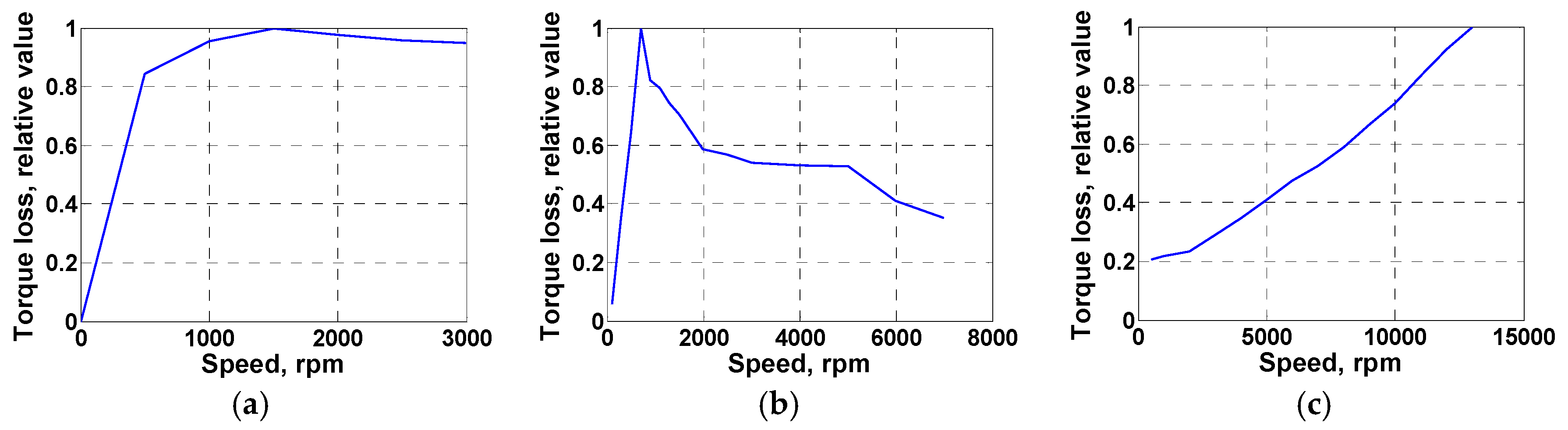
3.1.5. Seal Ring Loss

Seal rings are mounted at the transmission input and output shafts to block impurities and prevent oil leakage. Seal ring loss is caused by the friction between the shaft and lubrication oil film when rotating. A seal ring loss model was developed based on experimental results in Figure 4a. Seal ring loss increases with the rotational speed up to certain point and then maintains an almost constant value.

3.1.6. Brake Loss

Brake loss occurs due to the drag torque between the frictional surfaces when the brake is disengaged. It is known that the brake torque loss increases with the slip speed at relatively low slip speeds, and decreases at high slip speeds [32]. Brake loss was modelled using experimental results in Figure 4b.

3.1.7. MG1 Unloaded Loss

MG1 unloaded loss is generated by mechanical and electrical components when MG1 is freely rotating. For the target PHEV, even when MG1 is not working in EV#1 mode, it still has rotational speed because it is coupled to the vehicle speed through the PG (Figure 1). A MG1 unloaded loss model was developed based on experimental results in Figure 4c.

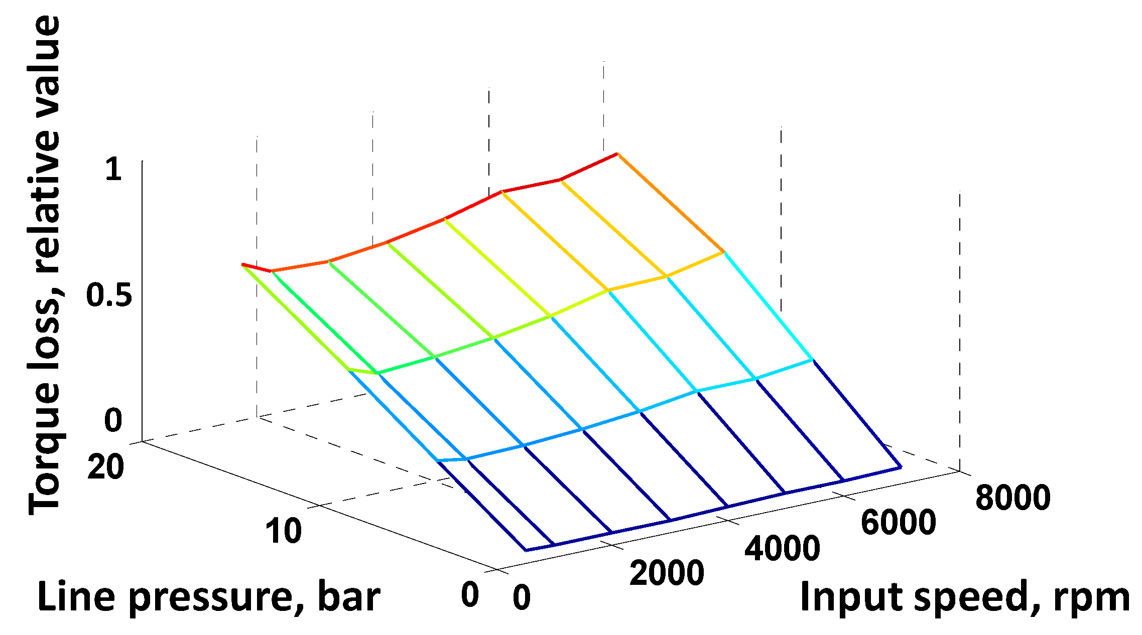
3.1.8. Oil Pump Loss

The oil pump supplies oil flow for lubrication, cooling, and brake control. In this study, a mechanical oil pump was used. Since the pump is connected to the drive shaft with an overdrive gear ratio, oil flow is supplied in proportion to the vehicle speed. The oil pump loss therefore depends on the vehicle speed and operating mode. In EV#1 and PS modes, oil flow is required only for the lubrication of mechanical components and cooling of the motor. In general, the lubrication oil flow increases with the rotational speed of the mechanical component. The oil flow for motor cooling depends on the motor temperature. In this study, it was assumed that the lubrication and cooling pressure was 1.5 bar. In EV#2 mode, additional oil flow is needed to control the brake engagement. For the target PHEV, the oil pump torque loss was obtained from the experimental results in Figure 5 [33].

3.2. Power Electronic System Losses

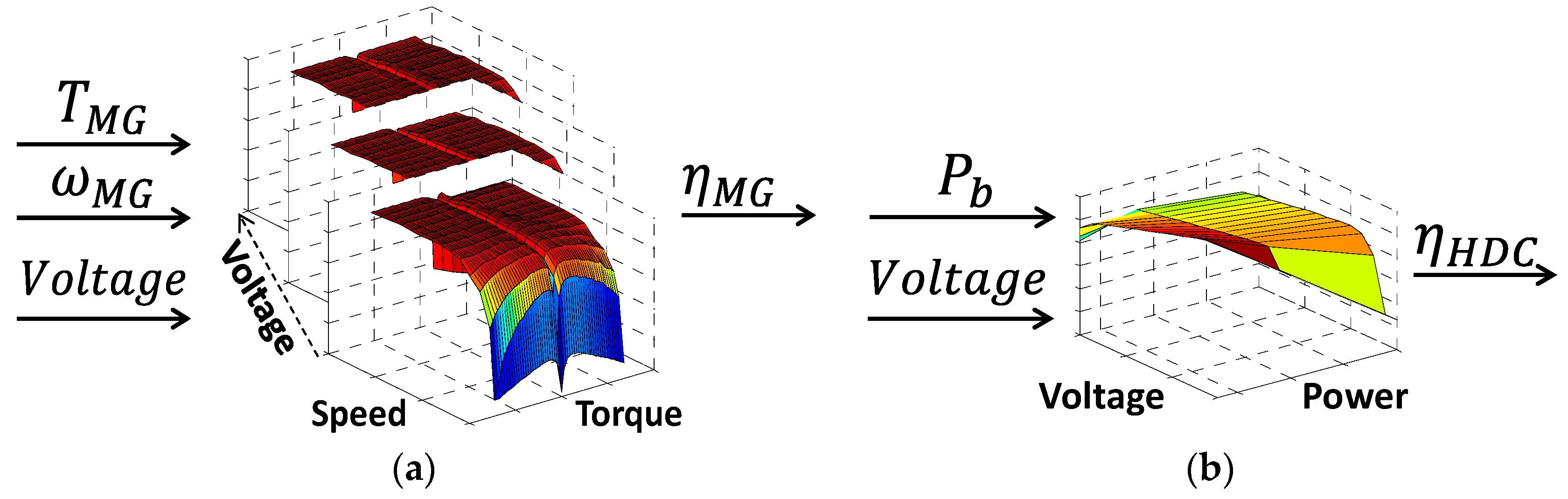
3.2.1. Motor-Generator Loss

The target PHEV system uses two motor-generators, MG1 and MG2. When MG1 or MG2 is motoring or generating, MG loss occurs due to the copper coil and iron core. Motor efficiency is determined from the motor output torque, speed, and input voltage. In this study, three input voltages were used from the high-voltage DC/DC converter (HDC). Bearing loss and inverter loss are also included in the MG efficiency map. A MG loss model was developed based on the MG efficiency as follows:

$$T_{\text{loss}\_\text{MGs}}=sign\left(P_{\text{mech}\_\text{MGs}}\right)\times \left({{\mathsf{\eta }}_{\text{MGs}}}^k-1\right)\times T_{\text{MGs}}\times {\mathsf{\omega }}_{\text{MGs}} k=\{\begin{array}{cc}-1,& \text{motoring}\\ 1,& \text{generating}\end{array}$$

(10)

where P_mech is the mechanical power, η is the efficiency. The MG efficiency map used in this study is shown in Figure 6a.

3.2.2. High-Voltage DC/DC Converter Loss

The HDC boosts the battery voltage according to the operating conditions of the MGs. HDC loss occurs from boost insulated-gate bipolar transistor (IGBT) loss (switching loss) and boost reactor loss [34]. As shown in Figure 6b, the HDC efficiency is determined by the battery power and input voltage of the MGs. HDC loss is then calculated from the HDC efficiency and battery power. An HDC loss model was developed using experimental results for the HDC output power.

4. Development of Dynamic Programming Backward Simulator with Drivetrain Losses

To develop an optimal mode control strategy taking into account drivetrain losses, a backward simulator was developed for the target PHEV using a DP algorithm. This is a global optimization problem to find the optimal engine and motor operation points which minimize fuel consumption for a given driving cycle while satisfying certain constraints. The global optimization process for the target PHEV has two control variables: engine speed and torque. Before performing global optimization for the whole driving cycle, local optimization was performed to reduce the number of control variables.

The goal of local optimization is to find the battery power which provides the minimum fuel consumption rate for the optimal engine operating points at each time stage [35]. From the instantaneous speed and torque of the engine, the drivetrain losses are calculated. Next, the admissible speed and torque of MG1 and MG2 (including the drivetrain losses) are determined from Equations (1) to (4), and the battery power P_b is determined from the MG1 and MG2 operating points:

$$P_{\mathrm{b}}={{\mathsf{\eta }}_{\text{MG}1}}^k\cdot T_{\text{MG}1}·{\mathsf{\omega }}_{\text{MG}1}+{{\mathsf{\eta }}_{\text{MG}2}}^k\cdot T_{\text{MG}2}\cdot {\mathsf{\omega }}_{\text{MG}2}, k=\{\begin{array}{cc}-1,& \text{motoring}\\ 1,& \text{generating}\end{array}$$

(11)

For the battery power obtained from Equation (11), all admissible points which satisfy the demanded wheel power can be determined. By comparing the fuel consumption rate at each admissible point, a local optimal engine operation point, ${{\mathsf{\omega }}^{*}}_{\mathrm{e}}$ and ${T^{*}}_{\mathrm{e}}$, can be obtained, as shown in Figure 7.

By finding the optimal point with the minimum fuel consumption rate among admissible engine operating points, P_b takes a one-to-one relation with the engine operating point. Repeating this process to find the battery power at different engine speeds and torques defines an instantaneous engine optimal line $h\left({{\mathsf{\omega }}^{*}}_{\mathrm{e}},{T^{*}}_{\mathrm{e}}\right)$ as [15]:

$$P_{\mathrm{b}}=h\left({{\mathsf{\omega }}^{*}}_{\mathrm{e}},{T^{*}}_{\mathrm{e}}\right)$$

(12)

where ${{\mathsf{\omega }}^{*}}_{\mathrm{e}}$ is the optimal engine speed, and ${T^{*}}_{\mathrm{e}}$ is the optimal engine torque.

Equation (12) shows that the optimization problem with two control variables (${{\mathsf{\omega }}^{*}}_{\mathrm{e}}$ and ${T^{*}}_{\mathrm{e}}$) can be reduced to an optimization problem with one control variable (P_b).

With the battery power P_b as the control variable, the state equation for the battery SOC can be represented as [21]:

$$\dot{SOC}=\frac{1}{C_{\text{bat}}}\frac{V_{\mathrm{b}}-\sqrt{{V^2}_{\mathrm{b}}-4R_{\mathrm{b}}{P}_{\mathrm{b}}}}{2R_{\mathrm{b}}}=f\left(P_{\mathrm{b}}\right)$$

(13)

where $\dot{SOC}$ is the time rate of change of the SOC, C_bat is the battery capacity, V_b is the battery output voltage, and R_b is the battery resistance. In this study, the battery output voltage V_b and internal resistance R_b are assumed to be constant.

Using these local optimization results, we can solve the global optimization problem to find the control variable (P_b) which has the minimum fuel consumption over the whole driving cycle. During the backward simulation, the global optimization process can be represented as a recursive equation consisting of a sequence of local optimization processes. The recursive equation and constraint for the global optimization problem can be expressed in discrete form as follows [21,36]:

$$\text{Recursive equation}: {J_k}^{*}\left(x_k\right)={{FC}^{*}}_k=\left\{g_{k-1}\left(P_b\left(k-1\right)\right)+{J_{k-1}}^{*}\left(SOC\left(k-1\right)\right)\right\}$$

(14)

$$\text{Constraint}:{SOC}_{\text{initial}}-{SOC}_{\text{final}}=0$$

(15)

where $k$ is the discrete time stage, ${J_{k-1}}^{*}$ is the optimal fuel consumption (g) from start to k − 1 stage, ${J_k}^{*}$ is the optimal fuel consumption from start to k stage, $g_{k-1}$ is the fuel consumption rate at k − 1 stage, and FC is the fuel consumption.

Through local and global optimization processes, the optimal control variable at every SOC at every time stage over the whole driving cycle can be obtained under the constraint that the final SOC is equal to the initial value. For the given SOC trajectory, the speed and torque of the engine, MG1, MG2, and drivetrain losses at every moment are also obtained.

5. A Rule-Based Mode Control Considering the Drivetrain Losses

5.1. Analysis of Drivetrain Losses and System Efficiency Using Dynamic Programming

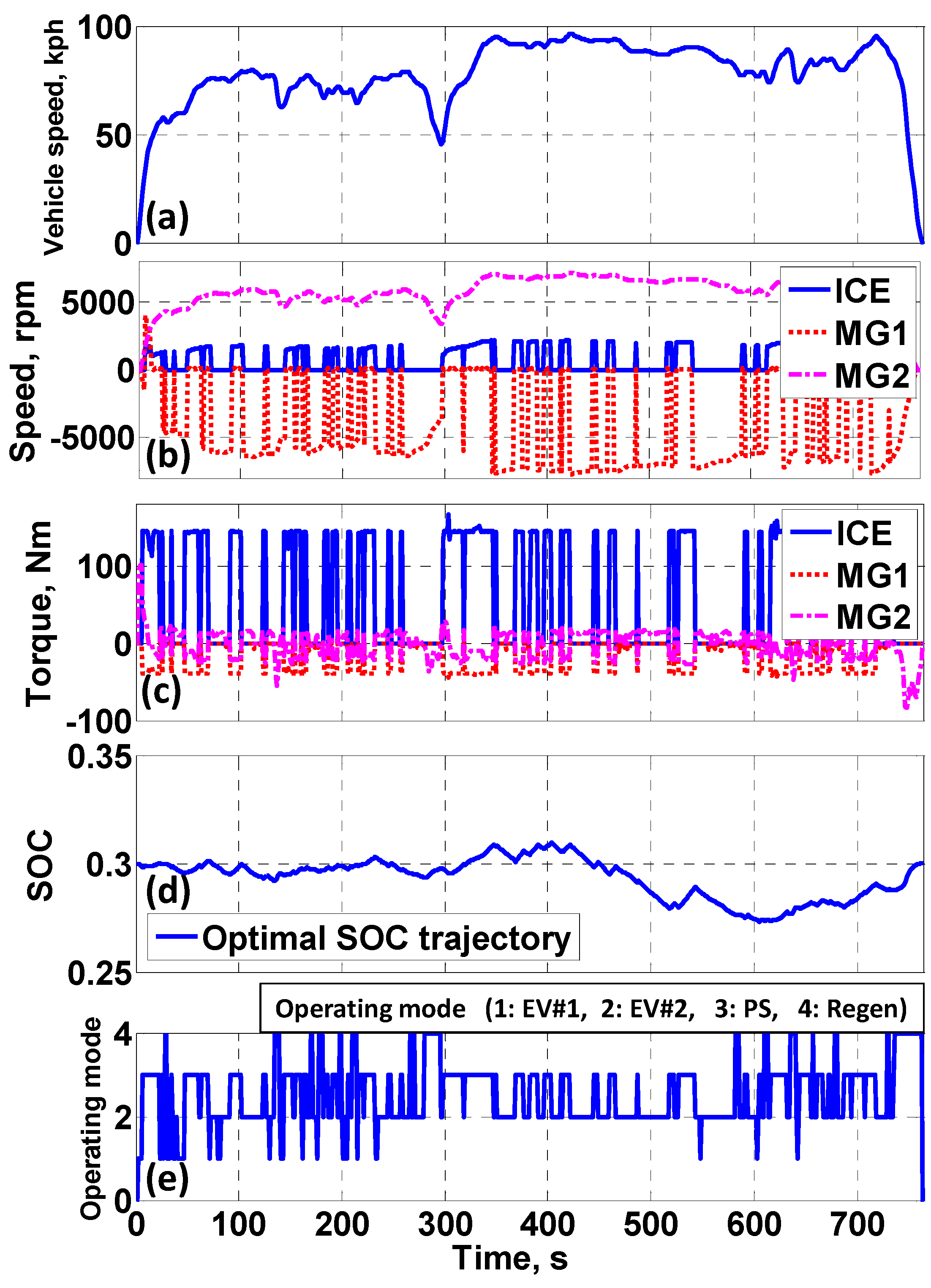
Using the powertrain model of the target PHEV and drivetrain losses, simulations were performed for urban dynamometer driving schedule (UDDS) and highway fuel economy test (HWFET) cycle driving cycles, with the constraint that the final battery SOC is equal to the initial SOC. To investigate the effect of including drivetrain losses on the mode control strategy, only the charge-sustaining (CS) mode of driving was simulated. In Figure 8, simulation results are shown for the HWFET cycle. The operating points—i.e., the speed and torque of the ICE, MG1, and MG2 which provide the minimum fuel consumption—were obtained using DP. The operating mode giving the minimum fuel consumption at every moment was then determined.

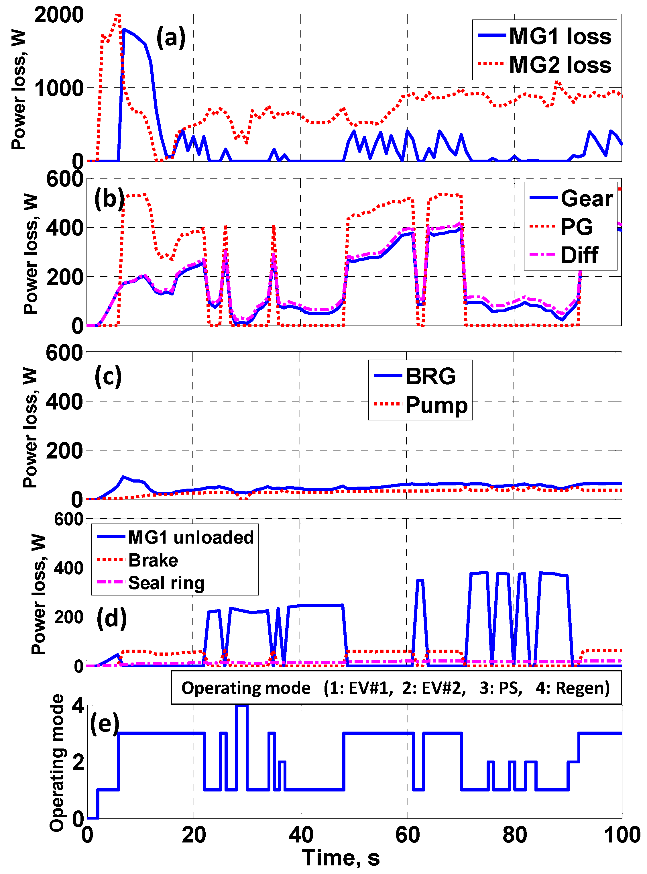
In Figure 9, MG1 and MG2 losses (Figure 9a) and drivetrain component losses (Figure 9b–d) are shown for t = 0–100 s of Figure 8. The MG2 loss is approximately 2000 W when the vehicle starts, and remains under 1000 W thereafter. Since MG2 acts as a main driving motor, the MG2 loss is larger than any other component and occurs whenever MG2 operates. MG1 has smaller loss than MG2 because MG1 is not a driving motor in the PS and EV#1 modes. The losses of the gear (Gear), PG, and differential gear (Diff) occur in proportion to the transmitted torque from the ICE, MG1, and MG2, and are in the range 0–500 W. Since the PG is connected to the ICE and the MG1 (Figure 1), PG loss occurs only when the ICE and MG1 are operated in the EV#2 and PS modes. The bearing (BRG) and pump losses are in the range 0–100 W. The MG1 unloaded loss, brake, and seal ring losses are a function of the speed. In the EV#1 and Regen modes, MG1 does not work. However, unloaded loss occurs in proportion to the vehicle speed, since MG1 is connected to the wheel through the PG (Figure 1). The MG1 unloaded loss is in the range 0–370 W. The brake loss is 0–140 W when the brake is disengaged in the PS mode. The seal ring loss depends on the speed and is 0–20 W.

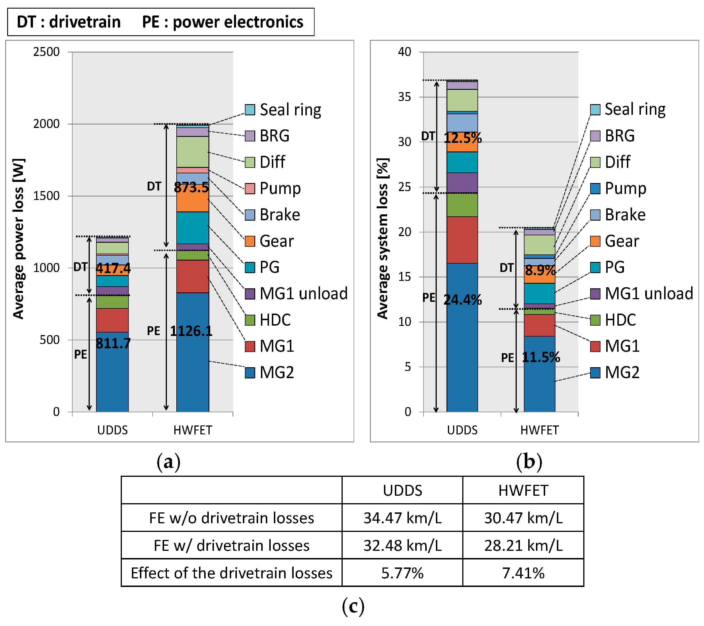
In Figure 10, the drivetrain losses and power electronics losses of the target PHEV are compared, and the effect of drivetrain losses on the fuel economy is investigated. It is seen from Figure 10a that the average power loss for the highway driving cycle (HWFET) increased compared with that of the city driving cycle (UDDS). This is because the power required to drive the HWFET cycle is larger, so the average power loss is also larger. As a percentage, the drivetrain losses reduce total system efficiency by 12.5% for UDDS and 8.9% for HWFET. The fuel economy with and without the drivetrain losses is compared in Figure 10c. It is seen that drivetrain losses reduce the fuel economy by 5.77%–7.41%.

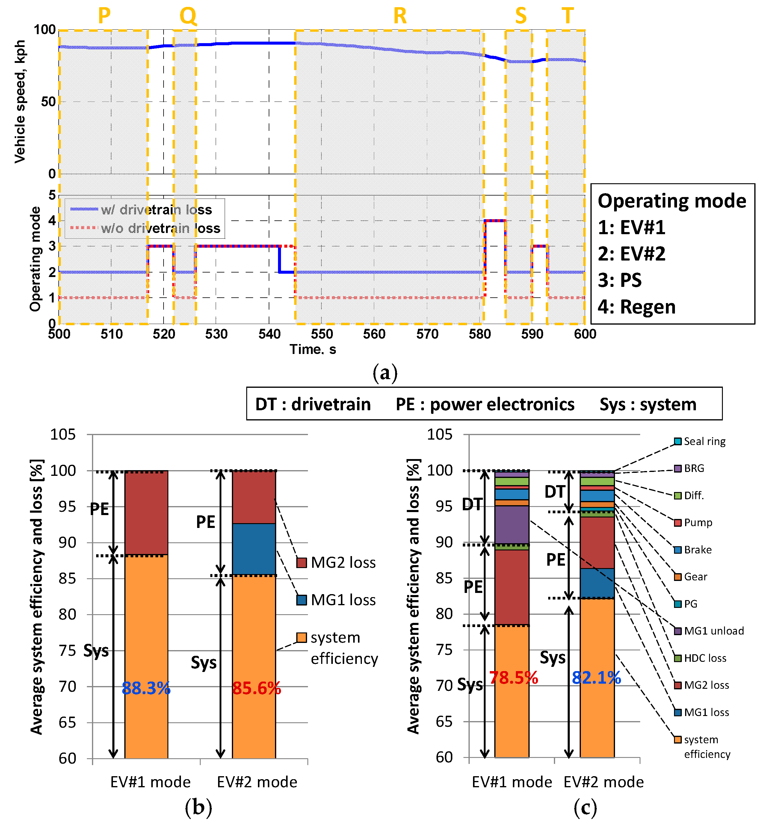
Next, we investigate the effect of drivetrain losses on the operating mode control strategy. In Figure 11a, the vehicle speed and operating mode are shown for the time range 500–600 s of HWFET. The target PHEV runs in EV#2 mode in the P, Q, R, S, and T regions when the drivetrain losses are included. On the other hand, the PHEV runs in EV#1 mode in the same regions when the drivetrain losses are not included. In Figure 11b,c, the average system efficiency and losses are shown for region R of Figure 11a. When the drivetrain losses are not included (Figure 11b), the average system efficiency in EV#1 mode is higher than in EV#2 mode because the power electronics losses in EV#2 mode are larger. On the other hand, when the drivetrain losses are included (Figure 11c), the system efficiency in EV#1 mode (78.5%) is lower than in EV#2 mode (82.1%). This is due to the MG1 unloaded loss which occurs when MG1 does no work in EV#1 mode. Therefore, the EV#2 mode has superior system efficiency in region R.

From the drivetrain losses analysis using DP in Figure 10 and Figure 11, we find that the optimum operating mode selection changes when drivetrain losses are included.

5.2. Rule-Based Mode Control Using the Dynamic Programming Results

Using a backward simulation which guarantees global optimality through DP, a RBC was developed for the presence or absence of drivetrain losses. As shown in Figure 11a, the operating mode that provides the highest system efficiency changes when the drivetrain losses are considered. In the Regions P, Q, R, S, and T, EV#2 mode is selected instead of EV#1 mode when the drivetrain losses are included. In Figure 11b,c, average system efficiency and losses are compared in EV#1 and EV#2 mode for the Region R of Figure 11a. It is noted that the system efficiency of EV#2 mode is higher than that of EV#1 mode when the drivetrain losses are included. As a result, EV#2 mode is selected instead of EV#1 in the Region R. The DP results in Figure 11 show that when drivetrain losses are considered, the operating mode which provides the highest system efficiency can change. To develop the RBC, the operating point corresponding to minimum fuel consumption was found at every moment for the entire city (UDDS) and highway (HWFET) driving cycles, and plotted with respect to wheel power and vehicle speed.

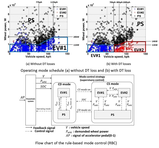
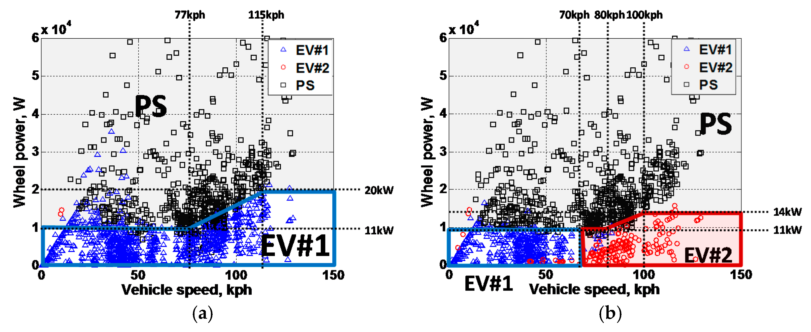
As shown in Figure 12a, when the drivetrain losses are not included, the EV#2 mode seldom appears in the operating range because the system efficiency of the EV#1 mode is higher than that of the EV#2 mode. It is seen from Figure 11b that the system efficiency of the EV#1 mode is higher due to the smaller PE loss when the drivetrain losses are not included. When the wheel power is less than 11 kW, the EV#1 mode is selected. At high vehicle speed, the EV#1 mode region is extended to a wheel power of 20 kW. Above the EV#1 mode region, the PS mode is selected.

When the drivetrain losses are included (Figure 12b), it is seen that the EV#2 mode appears in the low power, high speed region (0–11 kW, 70–80 kph or 0–14 kW, 100–150 kph). Therefore, the EV#2 mode is selected in this region. For the low power, low speed region (less than 11 kW, 70 kph), the EV#1 mode is selected. Above the EV#1 and EV#2 mode region, the PS mode is selected.

Using the mode control schedule obtained from DP, a rule-based control (RBC) was developed for the target PHEV with respect to the vehicle speed and wheel power. The flow chart of the RBC is shown in Figure 13. The wheel power, P_whl, can be determined from the accelerator pedal. Using the information of the present vehicle speed, V, battery SOC, and P_whl, the operation mode is determined as follows.

5.2.1. Charge-Depleting Mode

When the battery SOC is higher than the SOC lower limit, the vehicle is operated in EV#1 mode. If the wheel power is larger than the maximum battery power or the driver requires high performance such as rapid acceleration, the engine is activated and the vehicle runs in PS mode.

5.2.2. Charge-Sustaining Mode

Using P_whl and V, the operating mode is determined from the mode schedule in Figure 12.

For real-driving application of the RBC, a hysteresis region of ±500 W was established. Otherwise, the operating mode may change too frequently when the wheel power and vehicle speed are near the mode threshold boundary. Frequent mode changes between EV and PS modes cause frequent engine on/off switching, resulting in energy losses and unwanted emissions.

6. Target Plug-In Hybrid Electric Vehicle System Forward Simulator

6.1. Development of a Forward Simulator for the Target Plug-In Hybrid Electric Vehicle System

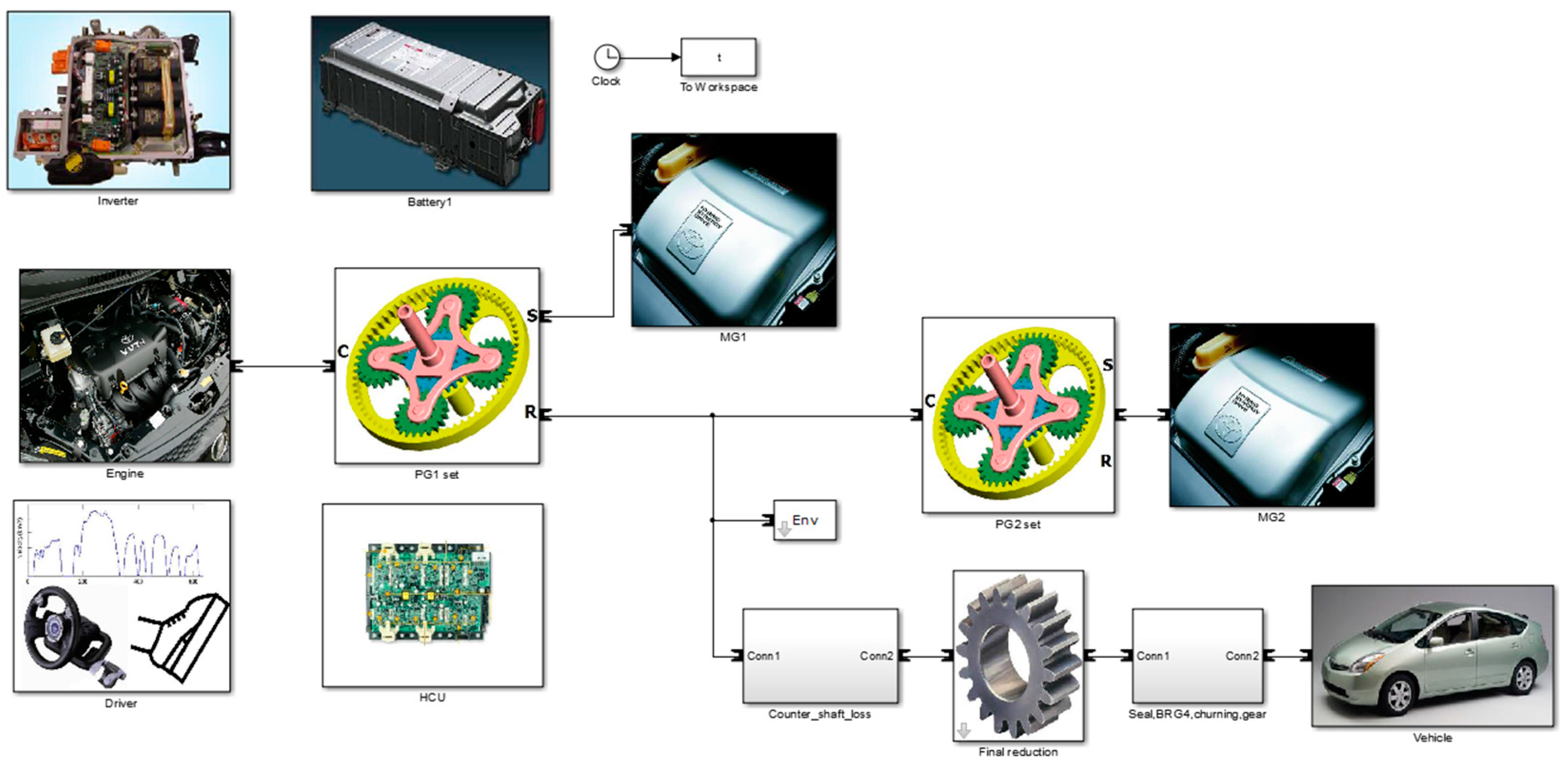
To evaluate the fuel economy of the target PHEV, a forward simulator was developed (Figure 14). In the forward simulator, dynamic characteristics such as the rotational inertia of driving components are considered, which could not be included in the backward simulation. Vehicle specifications used in the forward simulator are listed in

Table 2. Specifications for the target PHEV.

Engine	Capacity	115 kW
	Max speed	5700 rpm
	Max torque	211 Nm
MG2	Capacity	105 kW
	Max speed	13,000 rpm
	Max torque	270 Nm
MG1	Capacity	80 kW
	Max speed	13,000 rpm
	Max torque	59 Nm
Battery	Capacity	20 Ah
	Max power	50 kW
Transmission	PG ratio	2.4
	MG2 ratio	2.6
Vehicle	FGR	3.5
	Mass	1800 kg
	Tire radius	0.3 m

.

6.2. Investigation of the Forward Simulation Results

To evaluate the performance of the RBC developed in this study, simulations were performed in CS mode in the HWFET cycle and compared with the DP results, as shown in Figure 15. Vehicle speed (Figure 15a) by RBC followed the driving cycle closely. The RBC operating mode (Figure 15b) generally tracks that of the dynamic-programming-based control (DPC); however, there are some differences. One difference comes from the hysteresis of the RBC, which was introduced to prevent frequent mode changing. Due to the operating mode difference, the battery SOC (Figure 15c) is slightly different between DPC and RBC. In Figure 15d,e, the wheel power and operating mode are shown for t = 500–600 s (Region R in Figure 15a) of the HWFET cycle. In Figure 15d, the threshold power between the EV#2 and PS modes is plotted with the hysteresis. The threshold power was obtained using the vehicle speed and wheel power from Figure 12. As shown in Figure 15e, the operating mode changes twice between the EV#2 and PS modes for t = 515–545 s in the DPC. On the other hand, the mode change occurs only once in the RBC due to hysteresis. For t = 580–600 s, it is seen that regenerative braking was carried out when the vehicle speed decreased.

In

Table 3. Operating mode duration time and equivalent fuel economy (EFE) for the RBC and DPC in charge-sustaining (CS) mode under HWFET.

HWFET		RBC	DPC	Error (RBC/DPC)
Operating Mode Duration Time	EV#1	37 s	32 s	+15%
	EV#2	341 s	359 s	−5%
	PS	293 s	284 s	+3%
	Regen	93 s	85 s	+10%
EFE		27.4 km/L	28.2 km/L	−2.8%

, the operation time and fuel economy for RBC and DPC are compared for the HWFET driving cycle. The target PHEV is driven in EV#2 and PS modes for most of the driving cycle. The percentage error of the EV#2 and PS mode operation time is 5% and 3%, respectively. In the EV#1 and Regen modes, the percentage error is 10%–15%. However, since the operation times of EV#1 and Regen modes are relatively short compared with the total driving time, it is expected that the difference will not significantly affect the fuel economy. The fuel economy of the RBC was 27.4 km/L, lower than that of the DPC, which was 28.2 km/L. For this calculation, the equivalent fuel economy (EFE) was used, taking into account the difference in the final battery SOC. The error percentage of the fuel economy was 2.8%. However, considering that DPC is a purely theoretical approach, it is expected that the RBC developed in this study can provide near optimal control performance, which can be implemented in an on-line driving application.

Finally, using the RBC developed in this study, fuel economy was evaluated without drivetrain losses (Case 1) and with drivetrain losses (Case 2). For Case 1, the operating mode schedule obtained without considering drivetrain losses was used (Figure 12). As shown in

Table 4. Comparison of equivalent fuel economy by the RBC with and without the drivetrain losses.

Driving Cycle	Mode Control Strategy	EFE	Percent of Improvement in EFE
UDDS	Case 1: w/o DT losses	28.7 km/L	−
	Case 2: w/ DT losses	29.9 km/L	+4.1%
HWFET	Case 1: w/o DT losses	26.1 km/L	−
	Case 2: w/ DT losses	27.4 km/L	+4.9%

, the EFE of the RBC with drivetrain losses taken into account is higher than that of the RBC neglecting drivetrain losses by 4.1% and 4.9% for UDDS and HWFET, respectively. The EFE for UDDS is also higher than for HWFET because the energy recuperation by regenerative braking is larger, due to the frequent stop-and-go of city driving.

It is seen from the comparison that the RBC with drivetrain losses taken into account shows optimal performance nearly as good as the theoretically optimized DPC, and that drivetrain losses should be included in the development of mode control strategies in the design of PHEVs.

7. Conclusions

A near-optimal RBC was proposed for a target PHEV by considering the drivetrain losses. The target PHEV consists of an ICE, two MGs, one PG, and a brake, which implements three operating modes: EV#1, EV#2, and PS. First, to estimate the drivetrain losses, individual loss models were developed for each drivetrain component including the gears, PG, bearing, churning, seal ring, brake, and oil pump, based on experimental results and mathematical governing equations. A MG1 unloaded loss model was constructed to include loss generated when the MG1 is freely rotating. In addition, a power electronics system loss model was obtained considering the MG1, MG2, and high voltage DC/DC converter efficiency. To evaluate the effect of the drivetrain losses on the operating mode control strategy, backward simulations were performed using DP. Local optimization was carried out to reduce the number of control variables, and the battery power P_b was found for the instantaneous driving condition, which provides the minimum fuel consumption rate for the admissible engine operating points. With the battery power as a control variable, a state equation for the battery SOC was solved as a global optimization problem for the whole driving cycle. From the resulting SOC trajectory, the speed and torque of the ICE, MG1, and MG2, and the drivetrain losses were determined. By comparing the PHEV system efficiency, it was found that the operating mode selection is sometimes changed when the drivetrain losses are included. Using the DP results, an operating mode schedule was developed with respect to the wheel power and vehicle speed. It was found that the EV#2 mode seldom appears in the operating range when the drivetrain losses are not considered because the system efficiency of the EV#1 mode is better than that of the EV#2 mode. Based on the operating mode schedule, an RBC was developed, which can be implemented in an on-line application. To evaluate the performance of the RBC, a forward simulator was constructed for the target PHEV. From the simulation results, it was found that the RBC showed near optimal performance compared with the dynamic-programming-based mode control in terms of the mode operation time and fuel economy. The RBC developed with drivetrain losses taken into account showed a 4%–5% improvement in the fuel economy compared with the RBC that neglected the drivetrain losses.