Article

Insights on Energy Transitions in Mexico from the Analysis of Useful Exergy 1971–2009

1
Institute of Economic Research, National Autonomous University of Mexico, Circuito Mario de la Cueva s/n, Ciudad Universitaria, Mexico City 04510, Mexico
2
Marine, Environment and Technology Centre—MARETEC, Department of Mechanical Engineering, Instituto Superior Técnico, Universidade de Lisboa, Avenida Rovisco Pais, 1, Lisbon 1049-001, Portugal
*
Author to whom correspondence should be addressed.
Energies 2016, 9(7), 488; https://doi.org/10.3390/en9070488
Submission received: 30 April 2016 / Revised: 9 June 2016 / Accepted: 13 June 2016 / Published: 24 June 2016

Abstract

:
The analysis of useful exergy (UE), which is the minimum amount of work required to produce a given end-use, provides insights on the relationships between structural changes and energy transitions because it focuses on what energy is used for, i.e., energy services, rather than where it comes from, i.e., energy carriers. In this paper, UE was accounted for Mexico in 1971–2009. It was found that UE experienced a six-fold growth, led by the increasing share of mechanical drive and electric energy uses. Structural changes such as industrialization and complete electrification mainly drove UE transitions. Technological progress, mainly driven by the industrial sector, and electricity availability caused an improvement in the aggregate final-to-useful efficiency of the economy. In addition, the trend of increasing UE economic intensity shows that Mexico became more dependent on UE per unit of economic output during industrialization. The results suggest that UE trends were more influenced by structural transitions while final exergy trends were more influenced by economic fluctuations. It is concluded that energy policy design in developing countries undergoing or starting the process of industrialization should focus on: (1) improvements in final-to-useful efficiency, especially of the transportation sector and (2) growth of the productivity of UE.

1. Introduction

Energy transitions describe the changes in energy quantity and quality and the way in which energy carriers (“either a substance or a phenomenon that can be used to produce mechanical work or heat or to operate chemical or physical processes” [1]) are used in the economy [2,3]. These transitions, especially since the 18th century, are strongly related to wealth accumulation, population growth and improvements in the standard of living beyond Malthusian limits [4,5].
A fundamental characteristic of energy transitions is that they are endogenous to the economic system, which means that they are both caused and effected by structural changes in the economy, see e.g., Grubler [6], Kahrl and Roland-Holst [7], Feng et al. [8] and Rühl et al. [9]. Therefore, broader knowledge on these transitions may lead to adequate energy and environmental policies that boost sustainable development [10,11]. However, energy transition research has so far provided little understanding of economy-wide effects [12].
One reason for this little understanding is that most research studies have been mainly focused on the primary and/or final level of energy use (see Figure 1), e.g., Apergis and Payne [13], Recalde and Ramos-Martin [14], Chontanawat et al. [15], Costantini and Martini [16], Imran and Siddiqui [17], Jiang and Lin [18], and Wolde-Rufael [19]. Generally, these studies tend to overlook the productive role of energy within an economy (what it is used for) by focusing on energy sources (where it comes from) [20]. Consequently, energy uses are not taken into account, which is needed for a better evaluation of energy transitions [6,10,21].
Another reason is the predominance of energy-based analysis in the literature compared to exergy-based analysis. Energy-based analysis takes into account the thermodynamic potential of an energy carrier, e.g., enthalpy. On the other hand, exergy-based analysis focuses on the maximum work that is theoretically obtainable from an energy carrier as it approaches equilibrium with its environment, i.e., exergy [20]. The latter analysis, as opposed to the former, is directly related to energy quality and the processes of energy use; hence it should be preferred for policy-making [11].
Ayres and Warr [22], Warr et al. [23] and Warr, Ayres, Eisenmenger, Krausmann and Schandl [21], to complement conventional energy transition studies, proposed a methodology that accounts for useful exergy in the economy, focused on the final-to-useful conversion of exergy (Figure 1). This methodology was further developed by Serrenho et al. [24] and Serrenho et al. [25].
Useful exergy is the minimum amount of work required to produce a given end-use. It quantifies the effective amount of exergy that is delivered to a final function, e.g., the mechanical work from electricity used by a metal-bending machine or the exergy of the heat provided to an industrial process by a steam boiler.
The results from Warr, Schandl and Ayres [23], Warr, Ayres, Eisenmenger, Krausmann and Schandl [21] and Serrenho, Warr, Sousa, Ayres and Domingos [25] show that the distribution of useful exergy “is linked to structural changes in the demand of energy services.” It was also found that the final-to-useful exergy efficiencies improved due to an increase in energy quality, technology progress and structural shifts in the economy. These studies reported significant differences between the trends of useful exergy intensity (useful exergy/GDP) and final exergy intensity. Particularly, Serrenho, Warr, Sousa, Ayres and Domingos [25] found that useful exergy intensity in Portugal varied by only ± 20% around its 154-year average; while final exergy intensity experienced a stable decline.
The analysis of useful exergy, as suggested by the results of studies mentioned above, can also give further insights on the relationships between energy and economic growth, namely on energy decoupling. UNEP [26] defines energy decoupling as the reduction of the rate of use of primary energy per unit of economic activity, that is, reducing primary energy intensity; see also, Stern [5], Bithas and Kalimeris [27] and Ockwell [28]. Primary energy intensity can be linked to useful exergy intensity as follows:
P r i m a r y   e n e r g y G D P = ( P r i m a r y   e n e r g y F i n a l   e n e r g y ) 1 Φ f ( F i n a l   e x e r g y U s e f u l   w o r k ) ( U s e f u l   w o r k G D P )
The first term of Equation (1), which is the inverse of the aggregate conversion efficiency ( ν ) in Figure 1, depends on the structure of the energy sector and the characteristics of conversion processes from primary to final energy. The second term, which is the inverse of the aggregate exergy factor ( Φ f ), transforms final energy to final exergy. It depends on the energy carrier’s properties and the final energy mix of the economy. The third term, which is the inverse of the aggregate final-to-useful efficiency ( ε ), is related to energy use and the productive structure of the economy. Finally, the fourth term, the useful exergy intensity, is an indicator of the productivity of useful exergy. While the first three terms are subjected to thermodynamic limits ( ν and ε are necessarily bounded between 0 and 1), the fourth term is not. Therefore, reductions of useful exergy intensity can provide opportunities for further decoupling beyond thermodynamic limits, i.e., energy decoupling at the energy use level.
The present work accounts for useful exergy in Mexico between 1971 and 2009. The purpose is to understand energy transitions and identify related structural changes in the country. The focus is on the final and useful levels of energy use since these are directly linked to structural changes. The primary level of energy use is, therefore, not included.
Furthermore, this work is a contribution to the scarce and scattered specific research on Mexico’s energy transitions, which has been mainly focused on sectoral rather than economy-wide analysis, in a period where the country transitioned from a protectionist to a free trade economy. In this respect, Appendix A shows the main historical events during this period.
Sheinbaum et al. [29] evaluated the trends of Mexican residential energy use between 1970 and 1990. They found that electricity was the fastest growing end-use though the share of electricity in this sector was much smaller than that of oil products. Rosas et al. [30] analyzed the structure of household energy consumption between 1996 and 2006. They concluded that energy consumption for water heating and electric appliances significantly increased, while for cooking, it decreased; and that inequity in energy services among income groups grew.
Sheinbaum et al. [31] and Sheinbaum and Ozawa [32] studied the iron and steel industry in 1970–2006 and the cement industry in 1982–1994, respectively. They found that increases of energy efficiency and changes in the energy mix decreased the energy intensity in these industries. These improvements helped in reducing the gap in energy intensity with respect to best international practices. Moreover, Sheinbaum et al. [33] decomposed the driving factors of primary energy consumption of all manufacturing industries of the country between 1970 and 2008—An expansion and update of the analysis of Sheinbaum and Rodríguez [34]. They identified the structure of production and energy intensity as the main contributors to changes in energy use and CO2 emissions in most industries.
Berndt and Botero [35] in 1985 analyzed the energy demand of the transportation sector. Their main finding was that the effect of income on energy demand for transportation was larger than the effect of energy prices. In addition, Solís and Sheinbaum [36] evaluated the trends of energy consumption and CO2 emissions in the transportation sector in 1990–2010. They found that the increase of private vehicles and light truck transport were the main factors driving up the energy demand and emissions of the sector. They also found no correlation between fuel prices and energy consumption for the transportation sector.
Cheng [37] in 1997 applied the Granger causality test to Mexico’s primary energy consumption and economic growth aggregate variables and found no causal linkages between those variables. Galindo [38], through a co-integration approach, found that energy demand in Mexico over the period 1965–2001 was mainly driven by income and not by energy prices. Aguayo and Gallagher [39] gave insights on primary energy intensity in Mexico between 1965 and 1999. They found that it increased before 1988 and declined thereafter. According to their analysis, the decline was mainly caused by compositional factors and technological progress in the most energy-intensive industries. Furthermore, Sheinbaum et al. [40] examined the trends of energy demand and CO2 of five Latin American countries (including Mexico) from 1990 to 2006. They concluded that even though energy intensity decreased, the reduction of CO2 emissions was not significant due to an increased dependency of the primary energy mix on fossil fuels.
Finally, Ortiz [41] and Livas-García [42] analyzed the primary energy requirements of the Mexican economy for 1971–2007 and 1970–2010, respectively. The former found that the efficiency of the energy sector decreased mainly due to the rise of final demand for oil products. The latter concluded that the primary energy requirements of fossil fuels, especially natural gas, had a significant increase during the period under study.
This paper is organized as follows: Section 2 describes the methodology and presents details of its application to Mexico; in Section 3, aggregate results on useful exergy evolution, efficiencies and intensities are discussed; and, in Section 4, the main conclusions of the work are presented. In addition, Appendix A shows the main historical events during this period.

2. Experimental Section

This section describes the useful exergy accounting methodology (UEAM) and the materials and data handling for its application to Mexico in the period 1971–2009 (Supplementary Materials). The following subsections are ordered according to the steps of the UEAM by Serrenho, Warr, Sousa, Ayres and Domingos [25] (shown in Figure 2).

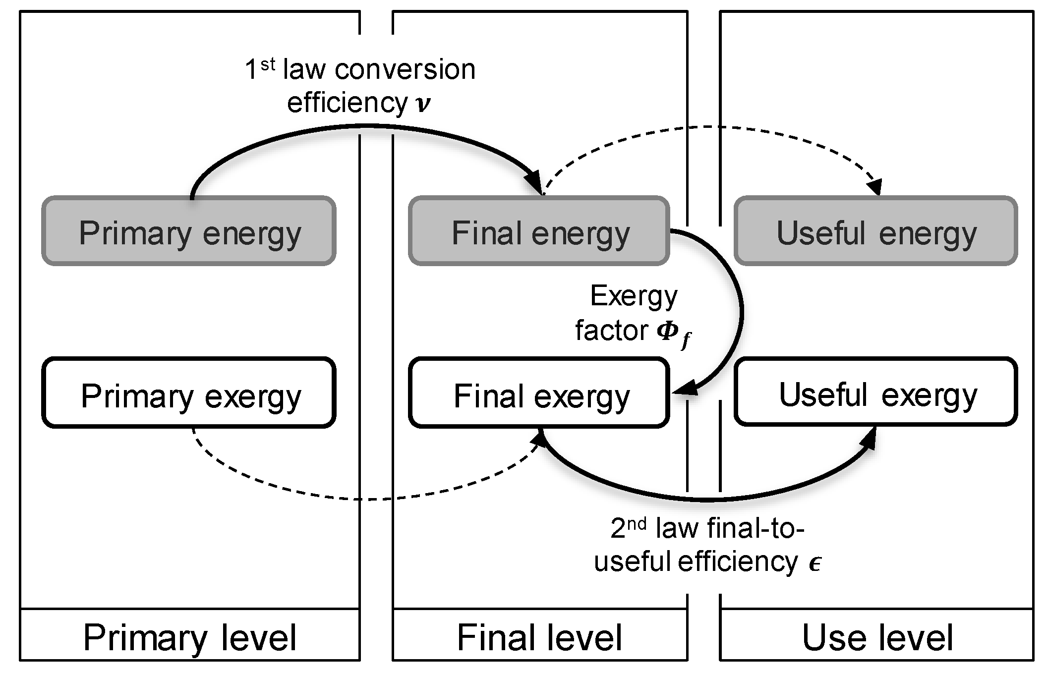
2.1. Conversion of Existing Final Energy Data to Final Exergy Values (Step 1)

2.1.1. Collecting Energy Data

Energy datasets are collected from available information of reliable institutions (e.g., International Energy Agency (IEA), World Bank, etc.). For a comprehensive accounting, data should include non-conventional energy carriers (exergy sources) such as food for humans, feed for draft animals and early renewables (e.g., wind for mills and boats), which had a significant role in the pre-industrialized era and in rural-based economies.
Final energy consumption data of Mexico were collected from the International Energy Agency’s Energy Statistics and Balances [43,44] and from the National Institute of Statistics and Geography (INEGI, for its Spanish acronym) [45,46,47] for the following energy carriers: Coal and coal products, Oil and oil products, Natural gas, Combustible renewables, Electricity, and Other non-conventional.
The sectoral classification of the IEA’s database was adopted for this work, which consists of 4 sectors (see Appendix B): Energy sector, industrial, transportation and others –including the residential, commercial, agricultural, forestry and public sub-sectors.
Consistency of data was evaluated by comparing IEA’s and INEGI’s data with each other. There were little variations between the two databases with respect to total final energy values per sector per carrier. However, INEGI’s data of the industrial and transportation sectors was preferred over IEA’s, since the latter presented inconsistencies in disaggregation.
Final food supply per capita as metabolizable energy data (defined as energy available for the organism’s use, e.g., heat production and body gains [48]) and as-is-weight livestock feed supply, which includes the total livestock, i.e., draft and non-draft animals, hence it was considered that the working animal share corresponds to a constant 10% of total livestock (this percentage was estimated by assuming Mexican working animal to total livestock ratio similar to that of Portugal in the 1960s. Data of total Mexican Livestock were obtained from INEGI [46] and USDA [49]. Data of Portuguese draft animals and total livestock were obtained from Henriques [2] and USDA [49] was collected from the FAO databases [50]).
Additionally, other economic indicators and variables, e.g., GDP per capita and demographics, were collected from IEA [43], INEGI [45], OECD [51] and The World Bank [52].

2.1.2. Conversion of Energy Data to Exergy Values

Conversions of energy ( E ) to exergy ( B ) values of energy carriers are given by a proportionality constant, called the exergy factor (Table 1), which is defined as:
Φ = B E
Final exergy values for Mexico, except for the food and feed carrier, were calculated by Equation (2), with final energy data and exergy factors from Table 1.
In the case of the food and feed carrier, the collected data was converted to final gross exergy values in the following way: Final food supply per capita as metabolizable energy was first multiplied by a gross/metabolizable ratio (Table 2) to obtain total gross exergy supply and then by an eaten/supplied ratio, which accounts for the amount of food that is not consumed. Furthermore, as-is-weight livestock feed supply was converted to gross exergy with Wirsenius’ [53] data for gross exergy of feed products. It is worth mentioning that FAO’s livestock feed data [50] does not include pasture hence pasture consumption was obtained from Wirsenius’s [53] figures of Latin-America and Caribbean countries’ feed and feedstock. Finally, the eaten/supplied ratio in Table 2 was applied.

2.2. Allocation of Each Final Exergy Consumption to One Useful Exergy Category (Step 2)

Final exergy consumption values per energy carrier are allocated to five useful exergy categories [25]:
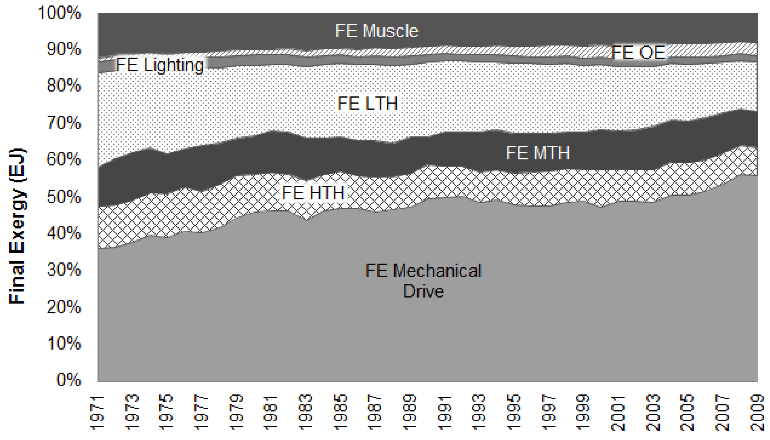
  • Heat: This category includes all heat used in the economy by processes and devices. It is subdivided in three types of use, based on temperature ranges of the hot reservoir [54]: (1) High temperature heat (HTH) (>600 °C) for most processes of heat-intensive industries such as iron, steel, cement, glass and oil refining industries [55]; (2) Medium temperature heat (MTH) (120–600 °C) for some processes of the metallurgical, chemical and energy industries [55], e.g., the digestion process of aluminum production; and (3) Low temperature heat (LTH) (<120 °C) for residential and industrial hot water, cooking and space heating and other low temperature industrial processes, e.g., pressing for paper production and canning for food preservation [55].
  • Mechanical drive: This category consists of mechanical work, which consists of any conversion to drive and movement by a mechanical device regardless of the final exergy carrier. Examples of this category are energy uses through internal combustion engines, electric motors and motors of household appliances (including those of HVAC and refrigeration; which are included in this useful work category because available data corresponds to the electricity consumption of their motors rather than to their heat extraction output. Even though a cooling useful work category, in theory, is more adequate for these devices, the estimation of heat extraction output from the electricity consumption data is unreliable).
  • Light: Includes the total lighting for industrial and residential use from any energy carrier. In modern/urban economies, most lighting services are produced by electricity. However, in developing/rural economies, lighting was also obtained from oil products, fat or “town gas”.
  • Other electric uses: This category includes others uses for electricity not mentioned in the previous categories. According to Serrenho, Warr, Sousa, Ayres and Domingos [25], this category is divided into two subcategories: (1) Communication, electronic and electric devices and (2) electrochemical processes.
  • Muscle work: Comprises useful exergy from ingested final gross exergy of food and feed by humans and animals, respectively.
Non-energy uses (i.e., all uses that do not specifically exploit the exergy content but other properties of a given energy source, for example, wooden furniture or oil derivatives, such as paints, lubricants and plastics) are not taken into account since, according to Ayres et al. [54], the share of final exergy for non-energy uses in the economy is several orders of magnitude smaller than for energy uses, hence negligible.
The allocation of final exergy uses in Mexico from IEA’s energy balances followed in general the assumptions for allocation by Serrenho, Warr, Sousa, Ayres and Domingos [25]. However, a few modifications were applied to account for Mexico’s specific conditions and available data. In the following sections, and in Appendix B, a description of the rationale for allocation by each energy carrier is presented.

2.2.1. Coal and Coal Products

High temperature processes of the metallurgical industries have accounted for most of the final consumption of coal over the studied period [56]. On the other hand, low temperature uses in the residential sector have been negligible [43] and uses for railroad transportation almost vanished due to the introduction of diesel technology before the 1970s [57].

2.2.2. Oil and Oil Products

Oil is fundamental for the economy and has had a significant impact on the economic performance in the last 40 years because it is the major contributor to government’s revenue and has accounted for a significant share of all Mexican exports since 1974, though with a decreasing trend: 68%, 37%, 10% and 16% in 1985, 1990, 2000 and 2011 respectively [45,58,59]. In particular, between 1973 and 1982, Mexico’s oil production notably increased from 150 to over 1000 million barrels a year [60]. Oil-fuelled motorization expanded and nowadays (this oil boom was caused by the Arab oil embargo of 1973, which caused a rise in oil prices [61] and hence boosted incentives to invest in the oil industry of non-OPEC countries).
The transportation sector accounts for the largest final demand for oil and its products. Automotive vehicles, as well as major automobile manufacturers, forayed into Mexico early in the 20th century [62,63]. Oil-fuel dominates freight and passenger transportation [36,64].
Demand of oil products (kerosene and oil lubricants) for residential uses, such as lighting and heating, were still significant in the second half of the 20th century due to the slow introduction of electricity. However, nowadays lighting residential oil uses have practically vanished over the studied period as the electric grid reached most households [45,65].

2.2.3. Natural Gas

Natural gas production has remained almost constant at about 14% of total energy production in the country during the entire studied period [43]. However, production did not cover total internal consumption, which made Mexico a net importer of natural gas from the United States since before the 1970s [66] (Valdez [67] infers that the low natural gas production with respect to reserves in Mexico is responsible for distortion and increases of natural gas prices in North America).
Industrial heating, mainly for MTH and HTH processes, held most of natural gas consumption before 2000 [68]. After that year, both industrial heating and electricity generation (non-final use) have led the demand of natural gas [43]. In addition, residential uses, which comprises low temperature heat for space, water and cooking, have been steadily rising [45].

2.2.4. Combustible Renewables

According to INEGI [45], two combustible renewables were mainly used in the period 1965–2011: sugar cane bagasse and wood for industrial and residential uses, respectively. Other sources, such as biofuels, waste and biogas were also used but in smaller quantities. However, data with respect to the residential sector are likely to be underestimated due to lack of information about biomass consumption in rural areas, which had 40% to 22% of the total population during the studied period [46,69].
Residential uses consist almost exclusively of LTH for cooking. On the other hand, industrial uses mainly correspond to MTH for sugar production, since bagasse is fed into boilers at ~280 °C [70]. In recent years, other combustible renewables have been included, e.g., biofuels for transportation (i.e., mechanical drive) and waste for electricity generation (non-final use) though their shares remain negligible.

2.2.5. Electricity

Electricity gained relevance over the studied period since the country completed electrification (measured by the percentage of total households in a country that have electricity [52]). In 1970, over 40% of the population remained without electricity. Further electricity generation/transmission projects were implemented boosting electricity access to 87% in 1990 and 98% in 2011 [45,65].
The allocation of final electric uses to useful exergy categories follows a sectoral analysis. The residential sector uses electricity for lighting, electric appliances and electronic equipment. Usually TV’s, radios and fridges lead consumption [71], except in urban areas where electronic devices are widely used and in regions with extreme climates where air conditioning is needed. In the case of the industrial sector, electricity is used for lighting, machinery, refrigeration, electronic appliances and air-conditioning. Detailed data of residential and industrial consumption are limited; only a few data points are available. Therefore, useful exergy shares were obtained by adjusting U.S. and U.K. estimates [72,73,74,75,76,77] according to available Mexican data points as described in Appendix C.
Finally, the transportation sector uses electricity mainly for subway transport systems, which started in the 1960s, and has had since a significant participation in the three most important cities [78]. However, electric transportation remains negligible in terms of total transportation energy use and total electric uses (<1%) [45].

2.2.6. Food and Feed

The final exergy of this carrier is entirely allocated to muscle work, useful exergy category provided to the economy by humans in the case of food and draft animals in the case of feed. Other uses by humans of food exergy, such as cognitive activities, are also allocated into this useful exergy category.

2.2.7. Other Non-Conventional

IEA’s databases include the contribution of solar thermal systems, which is used for low temperature water heating. In addition, other non-conventional carriers, such as wind flow to drive mechanical mills, are not accounted in databases since their contributions are negligible over the studied period.

2.3. Computation of Useful Exergy Values and Second-Law Final-to-Useful Efficiencies by Useful Exergy Category (Step 3)

Useful exergy values are obtained from the second law final-to-useful efficiencies and the allocated final exergy (see Figure 1) by:
U = ε · B
where B is the final exergy vector and ε is the second-law final-to-useful efficiency vector.
Second-law efficiency or exergy efficiency [79,80,81] represents the fraction of an exergy input that is converted into useful exergy. It measures the distance between results of real and ideal theoretical processes. Ford, Rochlin, Socolow, Hartley, Hardesty, Lapp, Dooher, Dryer, Berman, Silverstein and Ross [80] rewrote and provided detail to Equation (3) as:
ε = Minimum amount of work required to produce the desired energy transfer Maximum amount of work that could be produced from the relevant energy input
Exergy efficiency differs from energy efficiency or first-law efficiency ( η ) (defined as the ratio of desired energy transfer and the relevant energy input [80]) because the former gives a figure of merit, i.e., quality and closeness to ideal, and has a strict range of 0 ε 1 for any process of energy use, which allows the comparison between different processes. On the other hand, η does not provide a figure of merit and can take values larger than 1 for processes that involve an energy contribution from the environment (e.g., heat pumps).
Equation (3) shows that the values of second-law final-to-useful efficiency are needed to calculate useful exergy values. Therefore, in the following subsections, the definition and estimation of the second-law efficiencies for each useful exergy category are described. These values were then used to calculate the useful exergy estimates per carrier per economic sector and, ultimately, the useful exergy and efficiency figures by useful exergy category.

2.3.1. Estimation of Second Law Efficiencies for each Useful Exergy Category

a.
Heat
According to Ford, Rochlin, Socolow, Hartley, Hardesty, Lapp, Dooher, Dryer, Berman, Silverstein and Ross [80], ε h e a t is obtained through:
ε = Q 2 B ( 1 T 0 T 2 ) η ( 1 T 0 T 2 )
where η is the first-law efficiency, which represents the technological level of heat end-use devices (e.g., exchangers, furnaces, boilers, etc.); T 0 is the environment reference temperature, which refers to specific environmental conditions at the location where each heat conversion process is carried on; and T 2 is the temperature at which heat transfer occurs. The values of η , T 0 and T 2 for Mexico were obtained as follows:
The evolution of first law efficiencies ( η ) for most heat processes was estimated based on a representative industry for each temperature range and efficiencies of generic heat conversion devices [79]. For the HTH range, estimates were obtained from studies of the iron and steel industry [82,83,84]. In the case of the MTH range, the ammonia industry [85] and medium temperature processes of the iron industry [82,83] were used. For the LTH range, efficiencies were obtained from specifications of space heating devices from Cullen and Allwood [79] and Serrenho, Warr, Sousa, Ayres and Domingos’s [25] estimates.
Concerning the environment reference temperature ( T 0 ), as Mexico possesses a wide variety of climates, one yearly average temperature was calculated ( T 0 =   18.2 °C). This was done based on the yearly weighted average temperatures of the three main industrial regions: Centro, Norte and Bajio [86], and based on the assumption that each region has the same share of total heat uses since they had similar outputs of primary and secondary industries [87]. It is worth mentioning that the use of only one reference temperature does not significantly affect the accounting of useful exergy values, as found by Palma, Sousa and Guevara [81]. Finally, the temperature at which heat transfer occurs ( T 2 ) is defined within the limits of each heat sub- category (Table 3).
b.
Mechanical Drive
Gasoline engines, diesel engines and electric motors perform most of the mechanical work in every sector of the economy. Therefore, the second law efficiencies of these devices are considered. Gasoline engines: ε m e c h of these engines is obtained from that of the Otto thermodynamic cycle [80]:
ε η m a x i = 1 6 α i
where 0 α i 1 ,   i are coefficients that account for deviations from the ideal process and η m a x = 1 ( 1 / r ) r 1 , which is the maximum theoretical efficiency of the engine. It depends on the compression ratio ( r ) and the specific heat ratio γ = C p / C ν 1.4 .
Diesel engines: For the purpose of this work, ε m e c h for diesel motors can be considered 25% higher than that of gasoline engines since diesel engines have better compression ratios and better fuel-burning efficiencies [80]:
ε d i e s e l 1.25 · ε g a s o l i n e
Electric motors: ε m e c h is estimated from technical specifications and estimates in the literature, e.g., Ayres, Ayres and Pokrovsky [72].
In the case of Mexico, the values of the α i coefficients and the evolution of compression ratios were obtained from Ford, Rochlin, Socolow, Hartley, Hardesty, Lapp, Dooher, Dryer, Berman, Silverstein and Ross [80] and Serrenho, Warr, Sousa, Ayres and Domingos [25]. ε m e c h for electric motors and other mechanical equipment were estimated from engine specific information [79,88] and the evolution paths of the U.S. [21,25,72] since most equipment was imported from or manufactured according to standards of the northern neighbor.
c.
Light
Final-to-useful efficiency for a lighting technology differs from the others since it is determined based on a non-energy unit, i.e., lumens. It is defined as the ratio of generated lumens per watt by a lighting technology (e.g., kerosene lamp or a fluorescent bulb) and a reference value of maximum lumens per watt generated by an ideal light source:
ε = G e n e r a t e d   l i g h t   b y   a   l i g h t i n g   t e c h n o l o g y   [ l m / W ] R e f e r e n c e   l i g h t   g e n e r a t e d   b y   a n   i d e a l   l i g h t   s o u r c e   [ l m / W ]
Consequently, the useful exergy of a lighting technology represents the quantity of exergy that this ideal light source would consume to generate the same amount of lumens as those generated by the lighting technology. This approach to ε l i g h t is supported by most lighting and efficiency literature, e.g., Ayres, Ayres and Pokrovsky [72], Fouquet and Pearson [73] and Nordhaus [89].
Nevertheless, considerations about the value of the reference value in lumens per watt (ln/W) for 100% lighting efficiency differ: e.g., Ayres, Ayres and Pokrovsky [72] considered 400 ln/W, while Serrenho, Warr, Sousa, Ayres and Domingos [25] took 683 ln/W, associated to the wavelength of 555 nm (green light range) to which the human eye is most sensitive. For this study, the assumptions of Ayres, Ayres and Pokrovsky [72] are used.
Second law efficiencies for lighting in Mexico were obtained from U.S. estimated data [72]. To account for differences in economic development and infrastructure between of U.S. and Mexico, time-lags were applied to the data according to the characteristics of historical electric use in both countries, see Appendix C. Fouquet and Pearson’s [73] and Nordhaus’s [89] data were used for other energy carriers (such as kerosene) and for evaluating consistency of the results.
d.
Other Electric Uses
ε o t h e r   e l e c t r i c is calculated according to Equation (4). It accounts for the exergy losses of circuits and components of electric/electronic devices. This efficiency is estimated from available data and historical studies of second-law efficiencies of these devices, e.g., Ayres, Ayres and Pokrovsky [72]. Specifically, similarly to lighting, ε ’s of other electric uses in Mexico were adjusted based on U.S. estimates by Ayres, Ayres and Pokrovsky [72] as explained in Appendix C. In addition, estimates from Rosen and Bulucea [90] were used for evaluating consistency of adjusted data.
e.
Muscle Work
ε m u s c l e corresponds to the efficiency of human and animals to convert food and feed final gross exergy (which approximately corresponds to the maximum amount of heat obtained from complete combustion of a certain food in a bomb calorimeter [48]) into muscle work [25]. Therefore, ε m u s c l e accounts for incomplete absorption/digestion, for body growth and other body energy uses, for physiological state of the system, etc. [48].
Humans and animals have an efficiency to convert metabolizable energy from food and feed into useful muscle work with an efficiency of 17% and 21%, respectively [91,92,93]. The difference relies on the assumption that work performed by humans is half anaerobic and half aerobic; and by animals, mainly aerobic. To obtain the second law final to useful efficiency, this metabolizable-to-useful efficiency should be divided by a Gross/metabolizable ratio (Table 2), as:
ε m u s c l e = ( U s e f u l   e x e r g y M e t a b o l i z a b l e   e x e r g y ) ( G r o s s M e t a b o l i z a b l e ) = U s e f u l   e x e r g y F i n a l   g r o s s   e x e r g y

2.3.2. Obtaining Useful Exergy Values and Aggregate Second-Law Final-to-Useful Efficiencies for Each Useful Exergy Category

Having estimated specific second-law final-to-useful efficiencies, useful exergy values are computed with Equation (3). The second law efficiencies by category are calculated according to the share of final exergy by useful exergy sub-category:
ε = U s e f u l   e x e r g y   b y   c a t e g o r y   i T o t a l   f i n a l   e x e r g y   b y   u s e f u l   w o r k   c a t e g o r y   i

2.4. Calculation of Aggregate Useful Exergy Variables (Step 4)

Aggregate useful exergy figures and efficiencies for the whole economy are obtained from the results of previous steps. In addition, GDP in USD at constant prices and PPP’s data from IEA [44] were used to determine the useful exergy economic intensity as:
ε = U s e f u l   e x e r g y   b y   c a t e g o r y   i T o t a l   f i n a l   e x e r g y   b y   u s e f u l   w o r k   c a t e g o r y   i

3. Results

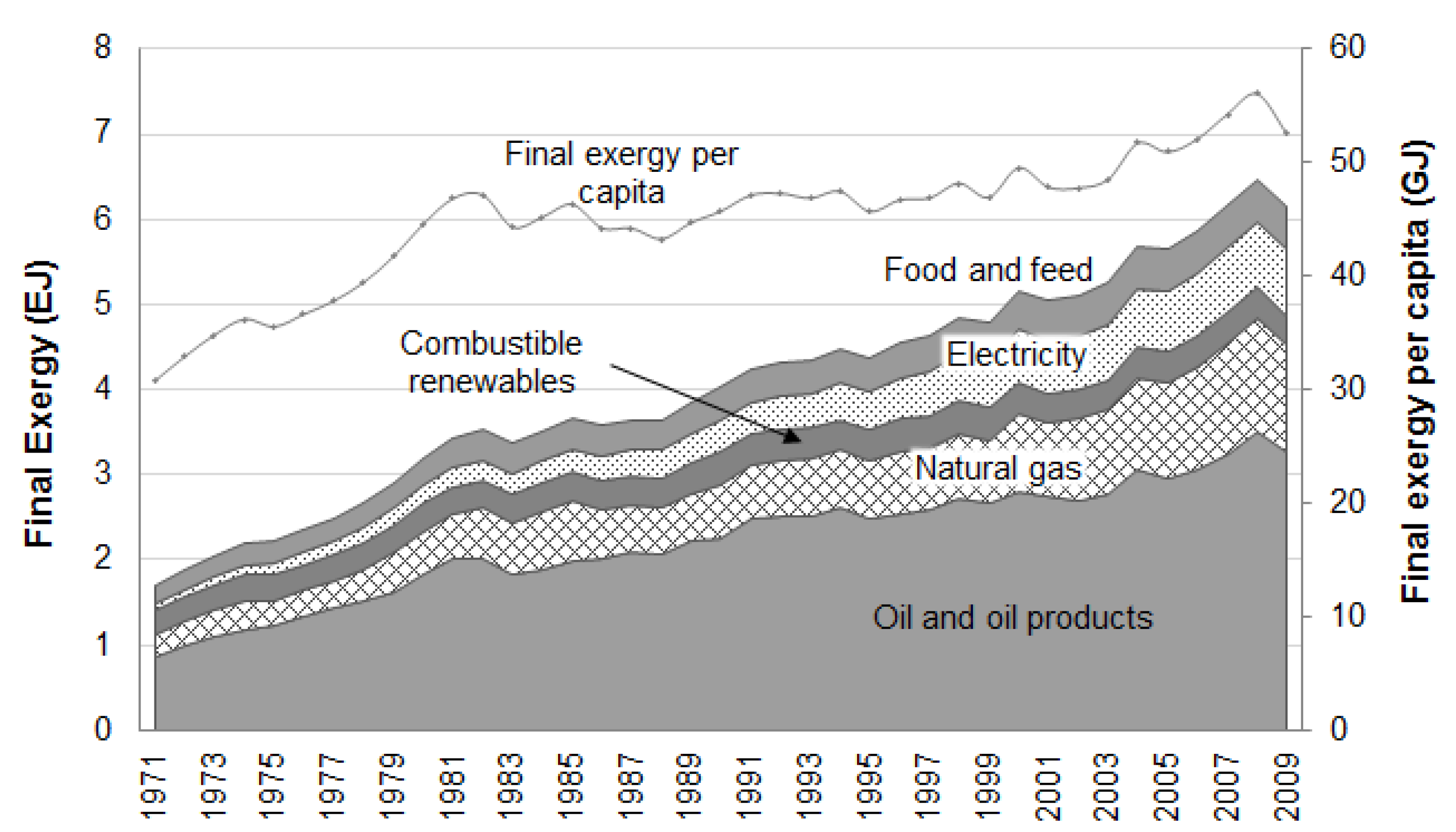
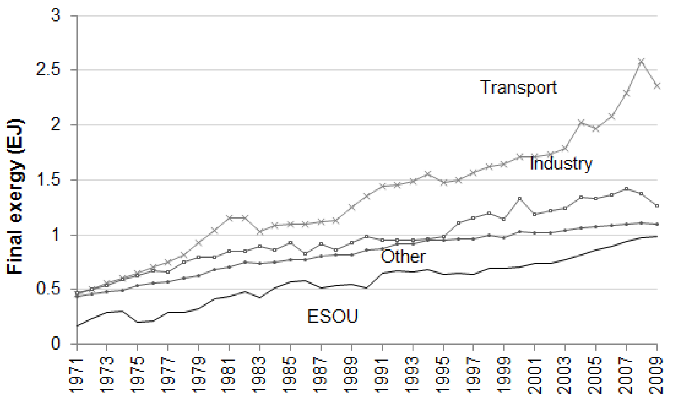
3.1. Final Exergy Trends

Mexico experienced a fourfold growth in final exergy consumption from 1.8 EJ to over 6 EJ in 40 years (Figure 3). The country had an average annual growth rate (AAGR) of final exergy demand of 3.4% (1.42% p/c).
During the studied period, Mexico underwent a radical transformation of its economic system. From an import-substituting economy, it became an open economy largely integrated with the U.S. However, the GDP’s AAGR in this period was 3.3%, a much poorer economic performance than in the previous period 1950–1970 when GDP had a 6% AAGR [94]. Import substitution industrialization consisted of government protection of heavy industries. The aim of the program was to develop these industries within borders, hence improving the country’s productive structure and reducing its imports. In Mexico, import substitution started early in the 1950’s and continued till the end of the 1970s [95,96,97,98].
In the interval 1971–1982, both final exergy use and per capita values were characterized by a large growth rate (AAGR 6.74% and 3.97% p/c). This was caused by: (1) structural changes and government investment in infrastructure brought by the oil industry boom [59]; (2) the sharp increase in final exergy use in the transportation sector (Figure 4); (3) productivity loss in non-oil industries [99]; and (4) the introduction/adaptation of heavy industries promoted by import substitution [97,98]. In the 1970s, the productivity of primary and secondary industries declined due to the tight government control over the economy and currency in the previous decades [100]. In 1976, the country faced economic slowdown, which did not continue because oil revenues compensated the effect of lost productivity. However, oil revenues gave a sense of economic stability, motivating public overspending, and increasing the flow of foreign revenues to the country, which boosted the so-called Dutch disease —sharp inflows of foreign income induce real exchange appreciation, which decreases the competitiveness of the main industrial sub-sectors compared with imports [99,101]. Finally, a sudden drop of oil prices ultimately led to the crisis of 1982 [59,94,102].
During 1982–1988, the growth rate of final exergy consumption slowed down (AAGR 0.57%, −1.43% p/c). This was caused by the economic crisis of 1982, which also led to the stabilization of the oil industry, the deceleration of the growth rate of final energy use by the transportation sector and the end of heavy industrialization by import substitution. In this interval, the country underwent important structural changes to allow for a less protectionist state. Even though the economic performance was poor, these changes enabled the opening of the economy in the subsequent period (1988–2001) [94,103].
The interval 1988–2001 was characterized by a larger growth rate of the final exergy demand (AAGR 2.49%, 0.77% p/c). Major changes in the country drove final exergy demand such as: (1) the abolition of import licensing [98,103]; (2) the North-American Free Trade Agreement (NAFTA) of 1994, which brought competition and productivity gains to previously protected industries; and (3) the privatization of many state-owned industries (including banks, rail, telecommunications, etc.) After NAFTA came into force, Mexico’s exports doubled and diversified [94]. From 1988, the Mexican government put emphasis on liberalizing the economy. The main proposal to achieve this goal was the free-trade agreement with the U.S., which was extended to include Canada. The government updated the institutions and regulation to enable the agreement. Foreign investment euphoria followed the announcement of NAFTA, large amounts of foreign capital flowed into the country. The latter fact led to a second version of the Dutch disease and to the 1994’s economic crisis. However, Mexico experienced a fast export-led recovery and by the end of 1995 the economy was again growing [94].
In 2001–2008, aggregate final exergy consumption had a larger growth rate (AAGR 3.57%, 2.3% p/c) mainly driven by the increase in exports and the rise of final exergy use by the transportation sector (Figure 4). Finally, the drop of aggregate final exergy consumption in 2009 was caused by the 2008’s world economic crisis that severely hit the U.S., the major commercial partner of Mexico. The main difference from the previous interval relies on the significant price increase of oil in 2001, which increased the share of oil exports compared to the 1990s and boosted public investment [59].
The trend of total final exergy use is largely influenced by the demand of final exergy by the transportation sector, which is the largest demand by sector (Figure 4). Road transportation accounted for over 90% of this demand. On the other hand, final exergy use by the industrial and other sectors steadily increased. Additionally, the ESOU reflects the status of Mexico as an oil exporter, i.e., oil extraction and refining accounted for more than 95% of the final exergy use of the energy sector.
The final exergy mix (Figure 5) shows a strong dependency of the economy on oil and natural gas. Oil and oil products accounted for half of total final exergy consumption while the natural gas share increased from 15% to 21%. Moreover, combustible renewables reduced their share by a half while electricity gained relevance from a 5% share in 1971 to 12% in 2000 as the country reached full electrification.
The final allocation of each final exergy consumption to useful exergy categories, according to Section 2.2, is shown in Figure 6. The share of final exergy for mechanical drive end-uses has increased from 36% in 1971 to 54% by the end of the period under study. Final exergy for LTH end-uses held a significant share, though decreasing from 24% to 11%. The share of final exergy for the MTH and HTH useful exergy categories remained almost constant in the period. Moreover, other electric uses increased their final exergy share while muscle and lighting slightly reduced it.

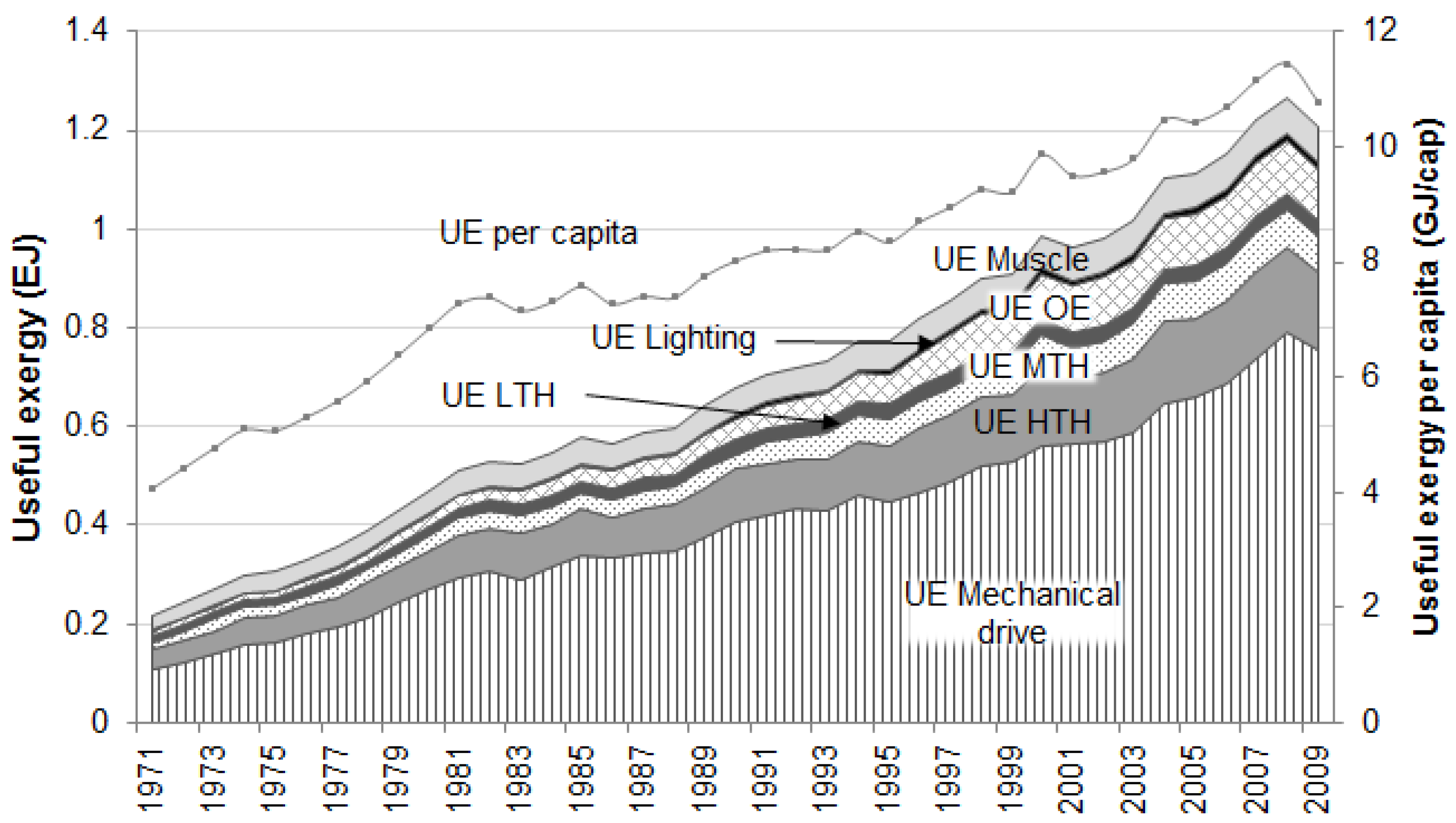
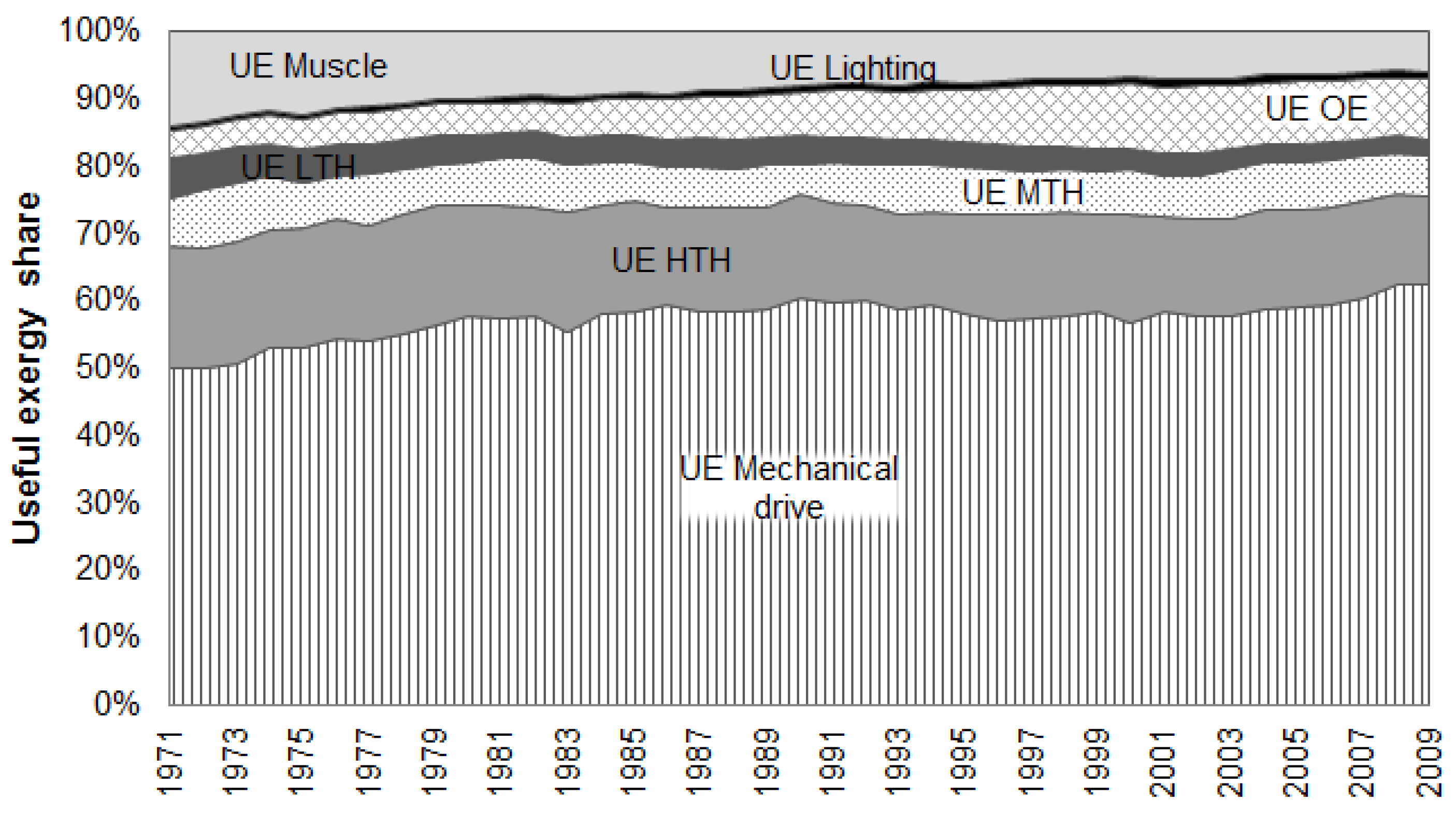
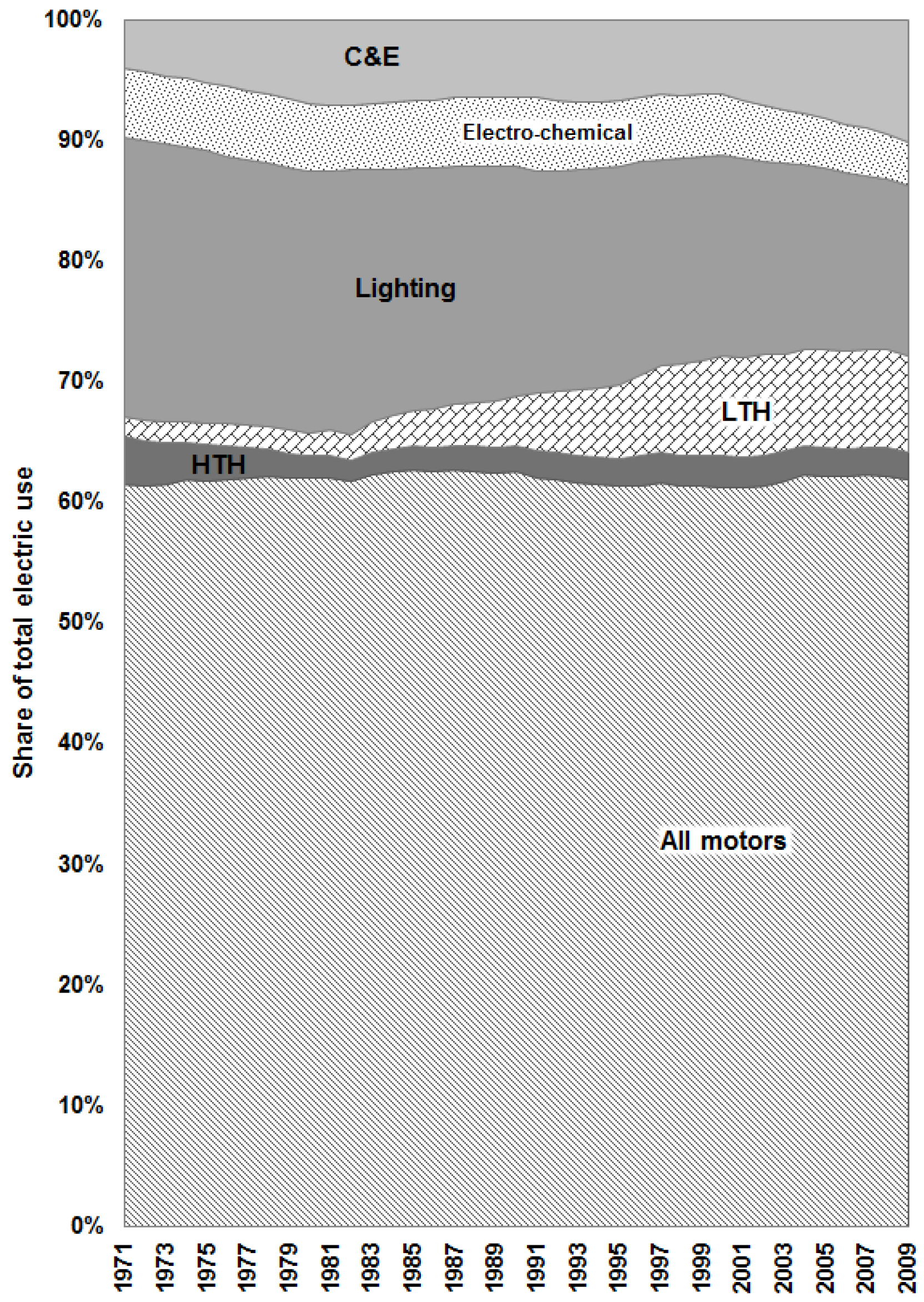
3.2. Useful Exergy Trends

Useful exergy reflects the evolution of exergy uses and services, which are influenced by structural changes of the economy. As seen in Figure 7, useful exergy had a six-fold growth from 0.2 EJ to 1.2 EJ over the studied period. The country had an AAGR of useful exergy demand of 4.49% (2.48% p/c).
The first interval (1971–1982) was characterized by a sharper rise (AAGR 8.22%, 5.35% p/c). As discussed before, this trend was caused by the development of the industrial structure, especially the oil industry, infrastructure projects and by the increase in transportation final exergy use. In 1982–1988, useful exergy slowed down (AAGR 1.99%, −0.04% p/c) while the country was struggling with the effects of 1982 economic crisis. The intervals 1988–2001 and 2001–2008, which are almost mutually indistinguishable, had a stable growth rate (AAGR 3.66% and 3.83%, respectively) associated to the transition towards an export-led economy.
The trend of useful exergy was highly influenced by the industrial sector, which held the largest share of useful exergy over the studied period (Figure 8); and, to a less extent, by the transportation sector, especially during the interval 1971–1982.
In the industrial sector, the trend in useful exergy experienced a stable growth, as shown in Figure 8. In the transportation sector, the trend in useful exergy is similar to the trend in final exergy (Figure 4). It is worth to mention that the useful exergy trends of the energy sector and the other sector had also stable but lower growth rates than the industrial and transportation sectors.
The shares of each useful exergy category are depicted in Figure 9. The role of mechanical work on the economy progressively increased in opposition to a decrease of the high temperature heat share. This was caused by growing energy needs for transportation (pure mechanical drive, see Figure 4) and an expansion of mechanical drive uses compared to high temperature heat uses in the industrial sector (mechanical drive uses in the industry increased six times by 2009 vis-a-vis its 1971s value, while high temperature heat increased less than four times [45]). The shares of medium temperature heat, low temperature heat and lighting uses remained almost constant. Moreover, the share of other electric uses also increased because of electricity availability and the deployment of electronic devices, especially in urban areas. Finally the share of muscle work was reduced by 50%, though it seems to have stabilized around 6% since 2005, which differs from the cases of Portugal and the UK (less than 2%) [25,104]. The latter is because of the lower degree of automation of Mexican industries, which means that Mexico is still more labor-intensive than developed economies.
The shares of useful exergy in Figure 9 differs significantly from the shares of final exergy by useful exergy category in Figure 6 due to the difference in second-law final-to-useful efficiency between useful exergy categories. The LTH useful exergy category had the largest difference, i.e., a share range of useful exergy of 2%–6% compared to a share range of final exergy of 11%–24%. The latter was caused by the low values of second-law final-to-useful efficiency of LTH end-use devices. On the other hand, the other electric uses category had a much larger share of useful exergy than of final exergy, especially after the 1990s. In addition, mechanical drive and HTH end-uses had a larger share of useful exergy than of final exergy.

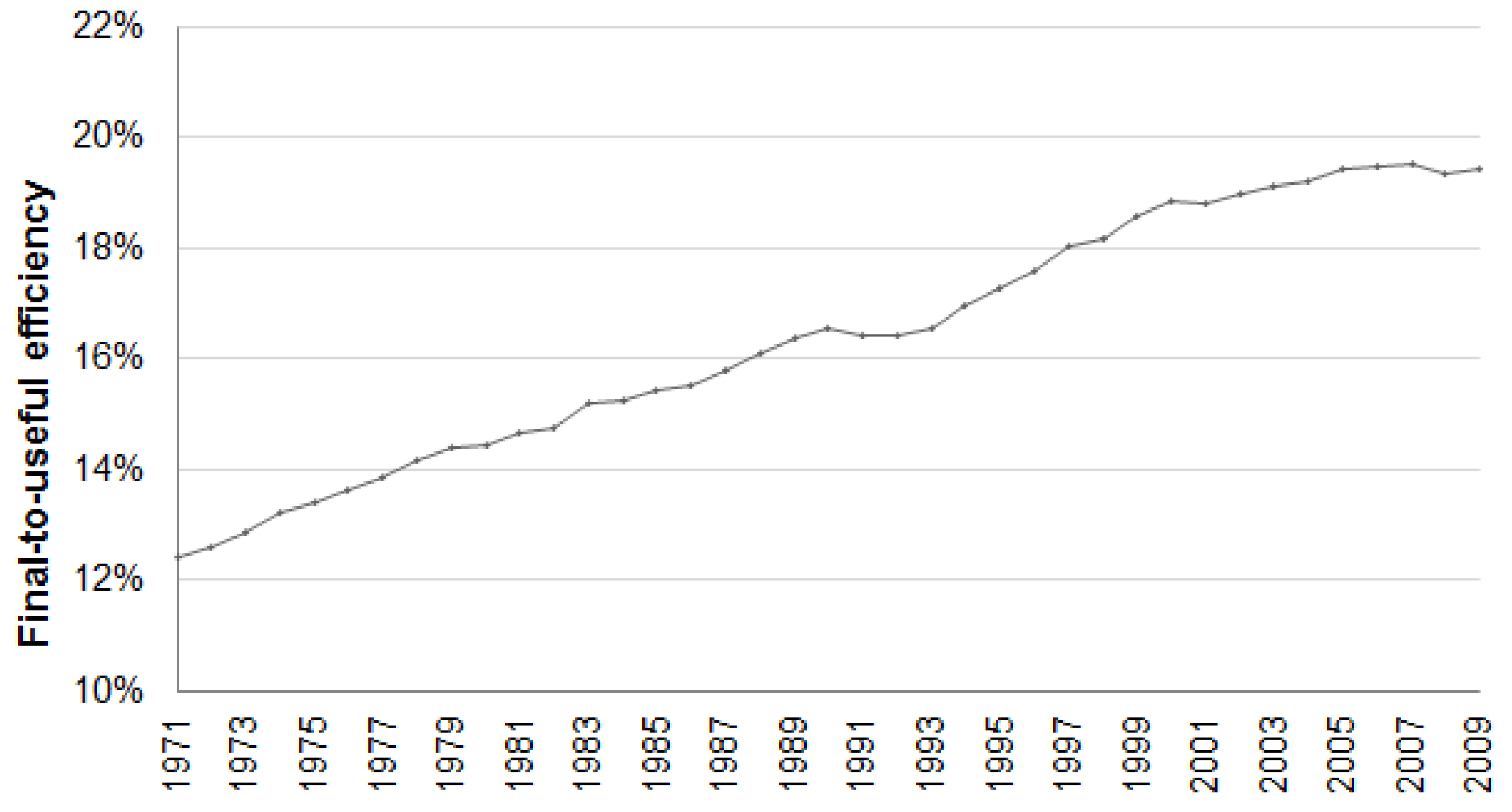
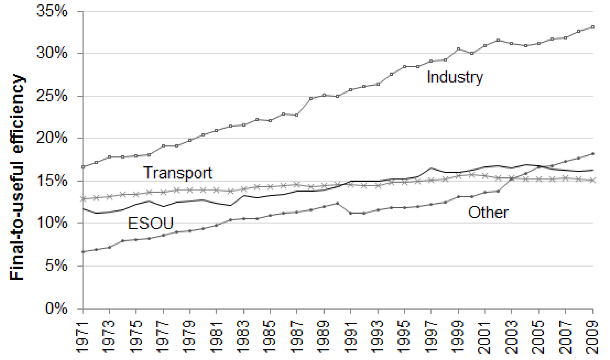
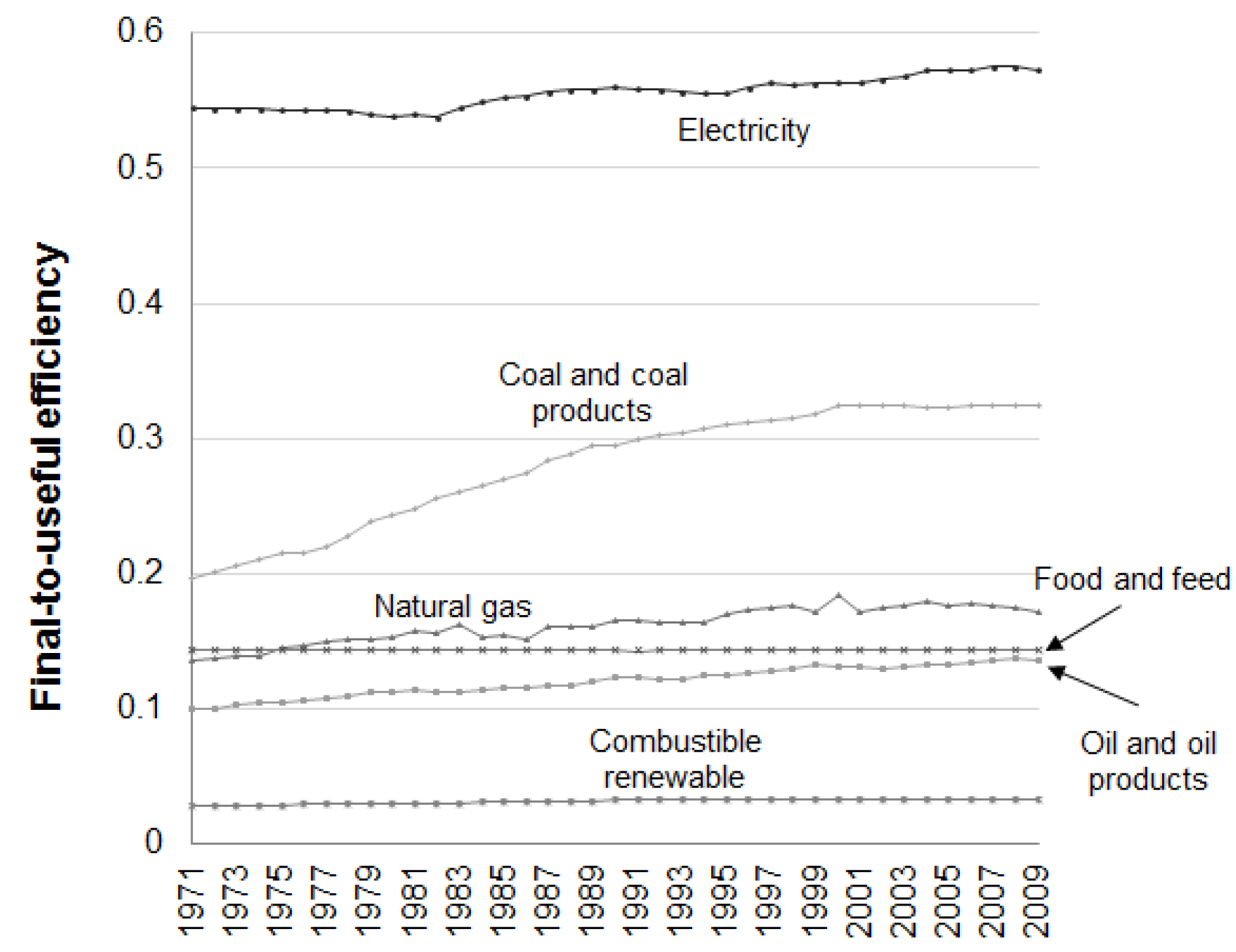
3.3. Final-to-Useful Efficiency

The aggregate second-law final-to-useful efficiency ( ε a g ) in Figure 10 represents the improvements that the structure of the Mexican economy went through during the studied period. It accounts for the larger increase of useful exergy (six-fold growth) compared to final exergy demand (fourfold growth).
Progress based on technological transfer from more developed countries, mainly U.S., brought more energy-efficient end-use devices and processes and partially led to an increasing trend of ε a g (13% to 19%). Two fluctuations from the trend are pointed out: (1) In (1982–1983), ε a g increased despite the economic crisis, which might be due to the closure of inefficient industries that could not endure the crisis; (2) In (1988–1994), ε a g declined due to the structural changes that the government undertook during those years. Later on, it increased again due to the productivity gains of an open economy.
The progress of ε a g was mainly driven by the industrial sector, which had the highest improvement on final-to-useful efficiency, i.e., 17% to 33% (Figure 11). On the other hand, the energy, transportation and other sectors also had improvements in efficiency, though much lower than the industrial sector. In addition, the small increase in the efficiency of the transportation sector (13% to 15%) explains the fact that this sector had a lower amount of useful exergy use compared to the industrial sector (Figure 8) even though it had the largest demand of final exergy (Figure 4).
Furthermore, the evolution of the final-to-useful efficiencies by energy carrier in Figure 12 shows that energy carriers were in general more efficiently used either by improvements in processes or carrier allocation to more efficient uses. Even though oil and oil products had a modest improvement in final-to-useful efficiency (9%–13%), this carrier accounted for a third of the increase in the aggregate second-law final-to-useful efficiency (Figure 10). Coal and coal product uses experienced the largest improvement of final-to-useful efficiency (20% to 32%, mainly due to the development of high temperature processes), though their impact was limited since this carrier accounted for less than 4% of total final exergy consumption. Moreover, the final-to-useful efficiency of natural gas shows an upward slope before 2000. After this year it stabilized because improvements of natural gas use by the industry were offset by the increase of low temperature heat residential uses, which have low efficiency [45]. Finally, electricity, which has the highest final-to-useful efficiency, shows a very moderate improvement. However, this carrier, whose share in the final energy mix increased from 5% to 12%, was fundamental for the increase of the aggregate second-law final-to-useful efficiency (Figure 10).

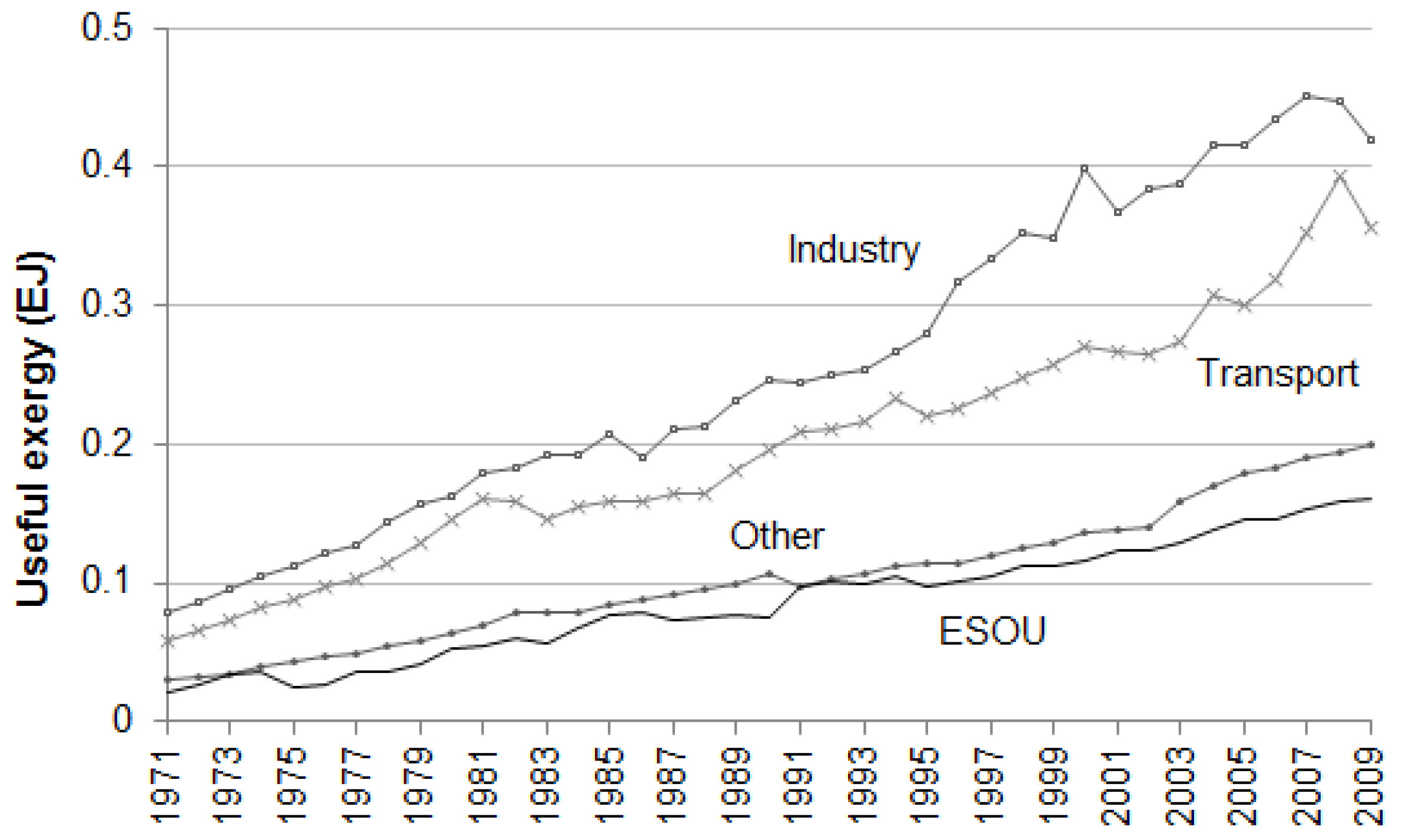
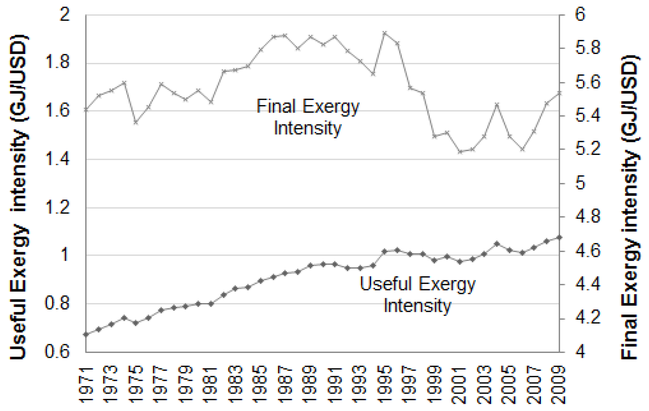
3.4. Useful and Final Exergy Trends

The useful exergy intensity of the economy had an increasing trend (Figure 13), which implies that the Mexican economy grew its minimum energy requirements to produce one unit of GDP. In other words, the economy became less productive per unit of useful exergy.
On the one hand, the upward trend of useful exergy intensity in a period in which Mexico was industrializing is congruent with what other economies experienced during industrialization such as U.S., Japan, U.K., Austria and Portugal [21,25]. In 1970–1988, the country unlocked the protectionist scheme in favor of a more opened economy, which increased useful exergy intensity by an AAGR of 1.78%. After 1988, most sectors of the economy opened, which induced a decline of the growth rate of useful growth intensity (AAGR 0.58%). This fact suggests that useful exergy intensity will eventually stop growing and even decline as it has happened in some of the countries mentioned above.
On the other hand, final exergy intensity (Figure 13) had a rather different trend, i.e., it varied ±10% from its 40-year average. In 1971–1982, it remained almost constant with a sharp decrease in 1975 as a prelude of the 1976 economic deceleration. After 1982, final exergy intensity rose under the economic stagnation before 1988. In most of the interval 1988–2001, the final exergy intensity decreased, except between 1994 and 1995, as a consequence of the 1994 crisis. The decline of final exergy intensity during this interval mainly reflect the efficiency gains and changes of composition of the industrial sector as concluded by Aguayo and Gallagher [39]. Finally, in 2001–2009, final exergy intensity experienced significant fluctuations, though with a slightly increasing trend (AAGR 0.78%).
The differences of final exergy and useful exergy intensities show that useful exergy intensity was more influenced by structural changes while final exergy intensity was more influenced by the economic fluctuations. Moreover, these differences also show that improvements of the aggregate final-to-useful efficiency had a positive effect on stabilizing final exergy intensity despite the rise of useful exergy intensity (see Equation (1)). These results confirm what Warr, Ayres, Eisenmenger, Krausmann and Schandl [21] and Serrenho, Warr, Sousa, Ayres and Domingos [25] found: the trends in useful exergy and final exergy intensities can be radically different.

4. Discussion and Conclusions

The dynamics of useful exergy in Mexico over the period 1971–2009 was characterized by a fourfold growth. The country increased its dependency on mainly mechanical drive and other electric uses due to structural changes such as industrialization, complete electrification, increase of transportation and broader use of electrical appliances.
Technological progress and the transition to energy carriers with more quality, i.e., electricity, led to a steady improvement in the aggregate second-law final-to-useful conversion efficiency of the economy. This improvement was mainly influenced by the industrial sector, which had the highest growth in final-to-useful efficiency compared to the energy, transportation and other sectors. Even though the transportation sector had the largest demand of final exergy, it experienced the lowest increase in sectoral final-to-useful efficiency. This was caused by small improvements in final-to-useful efficiency of gasoline and diesel engines (2% points) and by the small share of electricity use for transportation.
The results suggest that late stages of industrialization by import substitution, productivity losses in non-oil industries, the increase in final exergy use for transportation and the boom of oil production during the 1970s strongly influenced the trends of final exergy and useful exergy between 1971 and 1982. In the interval 1982–1988, final exergy and useful exergy were mainly affected by the structural changes the country underwent to face the 1982 economic crisis. After the year 1988, the changes of final exergy and useful exergy consumption were mainly influenced by the opening of the economy and its integration with the U.S. economy, which increased exports, brought productivity gains to most sectors of the economy and allowed a more diverse production in the country.
Final exergy intensity varied by ±10% from its 40-year average while useful exergy intensity increased. The differences of the evolution path of final exergy and useful exergy intensities show, on the one hand, that useful exergy intensity was more influenced by the structural transition from a generally protectionist to an export-led open economy and, on the other hand, that final exergy intensity was more influenced by economic fluctuations.
The upward trend of useful exergy intensity reflects that the economy became more dependent on useful exergy per unit of economic output over the studied period. However, the results also show that this increasing trend slowed down after 1990, which suggests that useful exergy intensity will eventually stop growing.
Energy policy design for developing countries undergoing or starting the process of industrialization need therefore to focus on: (1) improvements in the final-to-useful efficiency, especially of the transportation sector and (2) measures to increase the productivity of useful exergy, though further research is needed to understand and identify the factors that mostly influence the evolution of the useful exergy productivity. In addition, the substitution of fossil energy carriers to electricity for final energy uses can bring further improvements in the final-to-useful efficiency in every sector. However, this might not be true for the overall primary-to-useful efficiency as it also accounts for the conversion efficiency of electricity generation processes. Therefore, further research should also focus on including the three levels of energy use (primary, final and useful) into the analysis of energy transitions.

Supplementary Materials

The following are available online at www.mdpi.com/1996-1073/9/7/488/s1. Excel File: Useful exergy Mexico 1971 to 2009.

Acknowledgments

Work financially supported by Fundação para a Ciência e Tecnologia/MCTES (PIDDAC) through project UID/EEA/50009/2013. We would also like to thank the support of the MIT Portugal Program and Fundação para a Ciência e a Tecnologia through Ph.D. scholarship SFRH/BD/51297/2010 to Zeus Guevara.

Author Contributions

Tiago Domingos proposed the study, and controlled the quality of the results and the paper; Tania Sousa helped with the application of the methodology, and contributed to the interpretation of the results and the writing of the paper; and Zeus Guevara performed calculations, applied the methodology and wrote most of the paper.

Conflicts of Interest

The authors declare no conflict of interest.

Abbreviations

The following abbreviations are used in this manuscript:
UE
Useful exergy
UEAM
Useful exergy accounting methodology
HTH
High temperature heat
MTH
Medium temperature heat
LTH
Low temperature heat
ESOU
energy sector own use
GDP
Gross domestic product
PPP
Purchasing power parity
AAGR
Average annual growth rate
INEGI
National Institute of Statistics and Geography
IEA
International Energy Agency
FAO
Food and Agriculture Organization

Appendix A

Table A1 presents the main economic events during the period under study.
Table A1. 1971–2009 timeline.
IntervalYearEvents
1971–19821970sLast round of import substitution industrialization policies;
197040% of the population remained without electricity
1973Arab oil embargo
1974Beginning of the oil boom in the country
1976Economic deceleration; productivity loss in non-oil industries [99]
1977Large oil discoveries in the Gulf of Mexico
1982–19881980sEconomic stagnation
Policies to reduce protectionism [94,103].
1982Oil boom peak (1000 million barrels a year [60])
Sudden drop of international oil prices [59,94,102].
Economic crisis: Contraction of 0.5% and unemployment doubled
1983Banking system nationalization
1988–20011988–1994Abolition of import licensing [98,103]
Institutional updating for economic opening
199087% electricity coverage [45,65]
1994The North-American Free Trade Agreement (NAFTA)
1994–1995Dutch disease driven economic crisis
1995–1997Export-led economic recovery [94].
200098% electricity coverage [45,65]
2001–20082001Large surge in international oil prices
2001–2007Oil export driven increase in public investment
2008–20092008World economic crisis that severely hit the U.S., the major commercial partner of Mexico.

Appendix B

Table B1, Table B2, Table B3 and Table B4 show the assumptions for allocation to useful exergy categories of each energy carrier by sector. These assumptions were mainly estimated by Serrenho, Warr, Sousa, Ayres and Domingos [25] based on the sectoral information about processes, technology and efficiency from Harvey [55]. However, Serrenho’s et al. assumptions were complemented with the works of Ayres and Warr [20], Warr, Ayres, Eisenmenger, Krausmann and Schandl [21], De Beer, Blok and Worrell [83] and D’Angelo, Paz and Cardenas [70].
Table B1. Energy sector own use: Final exergy allocation assumptions.
Sub-SectorEnergy Carrier CategoryCarrier TypeUseful Exergy Category
Coal minesCoal and coal products MTH a
Oil and gas extractionOil and oil productsCrude oilMTH
Natural gas Mechanical drive
Electricity According to Appendix C
Coke ovensCoal and coal products HTH a
RefineriesOil and oil productsRefinery gasMTH
LPGMTH
Motor gasMechanical drive
DieselMechanical drive
Fuel oilMTH
BitumenMTH
Petro cokeMTH
Non-specifiedMTH
Natural gas MTH
Electricity According to Appendix C
Power producer plantsElectricity According to Appendix C
CHP and heat plantsElectricity According to Appendix C
Non-specified energyOil and oil productsKeroseneMTH
Electricity According to Appendix C
a HTH and MTH stand for high and medium temperature heat, respectively.
Table B2. Industrial sector: Final exergy allocation assumptions.
Sub-SectorEnergy Carrier CategoryCarrier TypeUseful Exergy Category
Iron and steelCoal and coal products HTH a
Oil and oil productsLPGHTH
KeroseneHTH
Gas dieselMechanical drive
Fuel oilHTH
Petro cokeHTH
Natural gas HTH
Electricity According to Appendix C
Chemical/petrochemicalOil and oil productsLPG50% HTH/50% MTH a
Gas dieselMechanical drive
Fuel oil50% HTH/50% MTH
Petro coke50% HTH/50% MTH
Natural gas 50% HTH/50% MTH
Electricity According to Appendix C
Non-ferrous metalsOil and oil productsLPG50% HTH/50% MTH
Gas dieselMechanical drive
Natural gas 50% HTH/50% MTH
Electricity According to Appendix C
Non-metallic mineralsCoal and coal products 50% HTH/50% MTH
Oil and oil productsGas dieselMechanical drive
Fuel oil50% HTH/50% MTH
Petro coke50% HTH/50% MTH
Natural gas 50% HTH/50% MTH
Electricity According to Appendix C
Transport equipmentOil and oil productsGas dieselMechanical drive
Fuel oil50% HTH/50% MTH
Natural gas 50% HTH/50% MTH
Electricity According to Appendix C
MachineryOil and oil productsLPG50% HTH/50% MTH
Gas dieselMechanical drive
Fuel oil50% HTH/50% MTH
Petro coke50% HTH/50% MTH
Mining and quarryingCoal and coal products 50% HTH/50% MTH
Oil and oil productsLPG50% HTH/50% MTH
Gas dieselMechanical drive
Fuel oil50% HTH/50% MTH
Natural gas 50% HTH/50% MTH
Electricity According to Appendix C
Food and tobaccoOil and oil productsLPGLTH a
Gas dieselMechanical drive
Fuel oilLTH
Combustible renewables LTH
Natural gas LTH
Electricity According to Appendix C
Paper, pulp and printingOil and oil productsLPGLTH
Gas dieselMechanical drive
Fuel oilLTH
Combustible renewables LTH
Natural gas LTH
Electricity According to Appendix C
ConstructionOil and oil productsGas dieselMechanical drive
Electricity According to Appendix C
Textile and leatherElectricity According to Appendix C
Non-specifiedCoal and coal products 50% HTH/50% MTH
Oil and oil productsLPG50% HTH/50% MTH
Kerosene50% HTH/50% MTH
Gas dieselMechanical drive
Fuel oil50% HTH/50% MTH
Petro coke50% HTH/50% MTH
Other non-conventionalSolar/windLTH
Combustible renewables LTH
Natural gas 50% HTH/50% MTH
Electricity According to Appendix C
a HTH, MTH and LTH stand for high, medium and low temperature heat, respectively.
Table B3. Transportation sector: Final exergy allocation assumptions.
Sub-SectorEnergy Carrier CategoryCarrier TypeUseful Exergy Category
RoadOil and oil productsLPGMechanical drive
Motor gasMechanical drive
DieselMechanical drive
Natural gas Mechanical drive
RailOil and oil productsDieselMechanical drive
Electricity Mechanical drive
Domestic navigationOil and oil productsDieselMechanical drive
Fuel OilMechanical drive
Domestic aviationOil and oil productsDieselMechanical drive
Fuel OilMechanical drive
Non specifiedOil and oil productsDieselMechanical drive
Table B4. Others sector: Final exergy allocation assumptions.
Sub-SectorEnergy Carrier CategoryCarrier TypeUseful Exergy Category
ResidentialOil and oil productsLPGLTH a
Kerosene70% Lighting/30% LTH before 1985 and 100% Lighting after
Natural gas LTH
Other non-conventionalSolar/windLTH
Combustible renewables LTH
Electricity According to Appendix C
Commerce/public servicesOil and oil productsLPGLTH
DieselMechanical drive
Fuel oilLTH
Natural gas LTH
Other non-conventionalSolar/windLTH
Electricity According to Appendix C
Agriculture/forestryOil and oil productsLPGLTH
KeroseneLTH
DieselMechanical drive
Electricity According to Appendix C
Non-specified (e.g., public lighting)Electricity According to Appendix C
a LTH stands for low temperature heat.

Appendix C

Disaggregate information about electric use in Mexico for the studied period is scarce and lacks detail. There are few data points available from reliable sources [105,106,107,108,109], hence studies focused on U.S. electric use [72,75] were used to estimate the allocation of electric use per economic sector.
Large differences exist between the productive structures, energy intensity and wealth of Mexico and the United States. However, due to their geographical proximity, technology, resources and capital have been flowing faster from the U.S. to Mexico in the past century than to other developing nations. Therefore, we assumed that the share of electricity use, as well as the final-to-useful efficiencies of the industrial, energy and other (except the residential) sectors (electricity uses by the transportation sector are negligible), have a 30-year lag when compared with those of the U.S. This value was defined by the years after 1970 that Mexico took to reach the level of full electrification [65]. The time lag was applied to Ayres, Ayres and Pokrovsky’s [72] data of U.S. shares and efficiencies of functional electric uses for the abovementioned sectors.
For the residential sector, we took a different approach, related to three variables: rural-to-urban population ratio, electricity access and ownership of household appliances. Based on these variables, data from U.S. were compared to Mexico’s [46,65,74,77]: Mexico lagged behind the U.S. in electricity access for about 40 years in 1960, though by 2010 it had caught up. In addition, the share of rural population in Mexico was 40% in 1970, which was the same as in the U.S. in 1940, yet by 2010 both countries had the same share of rural population (20% of the total population). Finally, regarding household indicators such as internet and computers penetration, a large difference remains, e.g., 76% compared with 25% in computer penetration in 2010, though this difference is exponentially decreasing [71,76]. Therefore, for the period 1940–2010, we assumed an initial time lag of 40 years in 1970 but decreasing linearly to 10 years by 2010 for residential electric uses. This 10-year lag accounts for the difference in household indicators. The time lag was applied to Ayres, Ayres and Pokrovsky’s [72] data of U.S. shares and efficiencies of functional electric uses for the residential sector.
Figure C1 shows the final estimates of functional electric use shares of total electric use for Mexico, which were built as done by [72].
The allocation of functional electric use into useful exergy categories is as follows: LTH, HTH and lighting electric uses are allocated to their homologous useful exergy categories. C&E and electrochemical electrical uses are allocated to other electric uses. Finally, All Motors belong to mechanical drive. Figure C2 shows the useful exergy share of total electric uses by useful exergy category.
Figure C1. Functional electric uses: Mexico 1971–2009. Note: HTH and LTH stand for high and low temperature heat, respectively. In addition, C&E stands for Communication and electronics.
Energies 09 00488 g014
Figure C2. Useful exergy of total electric use by useful exergy category: Mexico 1971–2009.
Energies 09 00488 g015

References

  1. International Organization for Standardization (ISO). Technical energy systems—Basic concepts. In ISO 13600; ISO: Geneva, Switzerland, 1997. [Google Scholar]
  2. Henriques, S.T. Energy Transitions, Economic Growth and Structural Change: Portugal in a Long-Run Comparative Perspective; Lund University: Lund, Sweden, 2011; Volume 54. [Google Scholar]
  3. Warr, B.; Ayres, R.U. Evidence of causality between the quantity and quality of energy consumption and economic growth. Energy 2010, 35, 1688–1693. [Google Scholar]
  4. Alam, M.S. Bringing energy back into the economy. Rev. Radic. Polit. Econ. 2009, 41, 170–185. [Google Scholar] [CrossRef]
  5. Stern, D.I. The role of energy in economic growth. Ann. N. Y. Acad. Sci. 2011, 1219, 26–51. [Google Scholar] [CrossRef] [PubMed]
  6. Grubler, A. Energy transitions research: Insights and cautionary tales. Energy Policy 2012, 50, 8–16. [Google Scholar] [CrossRef]
  7. Kahrl, F.; Roland-Holst, D. Growth and structural change in china’s energy economy. Energy 2009, 34, 894–903. [Google Scholar] [CrossRef]
  8. Feng, T.; Sun, L.; Zhang, Y. The relationship between energy consumption structure, economic structure and energy intensity in china. Energy Policy 2009, 37, 5475–5483. [Google Scholar] [CrossRef]
  9. Rühl, C.; Appleby, P.; Fennema, J.; Naumov, A.; Schaffer, M. Economic development and the demand for energy: A historical perspective on the next 20 years. Energy Policy 2012, 50, 109–116. [Google Scholar] [CrossRef]
  10. Rubio, M.d.M.; Folchi, M. Will small energy consumers be faster in transition? Evidence from the early shift from coal to oil in latin america. Energy Policy 2012, 50, 50–61. [Google Scholar] [CrossRef]
  11. Dincer, I. The role of exergy in energy policy making. Energy Policy 2002, 30, 137–149. [Google Scholar] [CrossRef]
  12. Dimitropoulos, J. Energy productivity improvements and the rebound effect: An overview of the state of knowledge. Energy Policy 2007, 35, 6354–6363. [Google Scholar] [CrossRef]
  13. Apergis, N.; Payne, J.E. Renewable energy consumption and economic growth: Evidence from a panel of OECD countries. Energy Policy 2010, 38, 656–660. [Google Scholar] [CrossRef]
  14. Recalde, M.; Ramos-Martin, J. Going beyond energy intensity to understand the energy metabolism of nations: The case of argentina. Energy 2012, 37, 122–132. [Google Scholar] [CrossRef]
  15. Chontanawat, J.; Hunt, L.C.; Pierse, R. Does energy consumption cause economic growth?: Evidence from a systematic study of over 100 countries. J. Policy Model. 2008, 30, 209–220. [Google Scholar] [CrossRef]
  16. Costantini, V.; Martini, C. The causality between energy consumption and economic growth: A multi-sectoral analysis using non-stationary cointegrated panel data. Energy Econ. 2010, 32, 591–603. [Google Scholar] [CrossRef]
  17. Imran, K.; Siddiqui, M.M. Energy consumption and economic growth: A case study of three saarc countries. Eur. J. Soc. Sci. 2010, 16, 206–213. [Google Scholar]
  18. Jiang, Z.; Lin, B. China’s energy demand and its characteristics in the industrialization and urbanization process. Energy Policy 2012, 49, 608–615. [Google Scholar] [CrossRef]
  19. Wolde-Rufael, Y. Energy demand and economic growth: The african experience. J. Policy Model. 2005, 27, 891–903. [Google Scholar] [CrossRef]
  20. Ayres, R.U.; Warr, B. The Economic Growth Engine. How Energy and Growth Drive Material Prospertity; Edward Elgar: Cheltenham, UK, 2009. [Google Scholar]
  21. Warr, B.; Ayres, R.U.; Eisenmenger, N.; Krausmann, F.; Schandl, H. Energy use and economic development: A comparative analysis of useful work supply in austria, japan, the united kingdom and the us during 100 years of economic growth. Ecol. Econ. 2010, 69, 1904–1917. [Google Scholar] [CrossRef]
  22. Ayres, R.U.; Warr, B. Accounting for growth: The role of physical work. Struct. Change Econ. Dyn. 2005, 16, 181–209. [Google Scholar] [CrossRef]
  23. Warr, B.; Schandl, H.; Ayres, R.U. Long term trends in resource exergy consumption and useful work supplies in the uk, 1900 to 2000. Ecol. Econ. 2008, 68, 126–140. [Google Scholar] [CrossRef]
  24. Serrenho, A.C.; Sousa, T.; Warr, B.; Ayres, R.U.; Domingos, T. Decomposition of useful work intensity: The EU (European Union)—15 countries from 1960 to 2009. Energy 2014, 76, 704–715. [Google Scholar] [CrossRef]
  25. Serrenho, A.; Warr, B.; Sousa, T.; Ayres, R.U.; Domingos, T. Structure and dynamics of useful work along the agriculture-industry-services transition: Portugal from 1856 to 2009. Struct. Change Econ. Dyn. 2016, 36, 1–21. [Google Scholar] [CrossRef]
  26. United Nations Environment Programme (UNEP). Decoupling Natural Resource Use and Environmental Impacts from Economic Growth; UNEP: Paris, France, 2011. [Google Scholar]
  27. Bithas, K.; Kalimeris, P. Re-estimating the decoupling effect: Is there an actual transition towards a less energy-intensive economy? Energy 2013, 51, 78–84. [Google Scholar] [CrossRef]
  28. Ockwell, D.G. Energy and economic growth: Grounding our understanding in physical reality. Energy Policy 2008, 36, 4600–4604. [Google Scholar] [CrossRef]
  29. Sheinbaum, C.; Martínez, M.; Rodríguez, L. Trends and prospects in Mexican residential energy use. Energy 1996, 21, 493–504. [Google Scholar] [CrossRef]
  30. Rosas, J.; Sheinbaum, C.; Morillon, D. The structure of household energy consumption and related CO2 emissions by income group in Mexico. Energy Sustain. Dev. 2010, 14, 127–133. [Google Scholar] [CrossRef]
  31. Sheinbaum, C.; Ozawa, L.; Castillo, D. Using logarithmic mean divisia index to analyze changes in energy use and carbon dioxide emissions in Mexico’s iron and steel industry. Energy Econ. 2010, 32, 1337–1344. [Google Scholar] [CrossRef]
  32. Sheinbaum, C.; Ozawa, L. Energy use and CO2 emissions for Mexico’s cement industry. Energy 1998, 23, 725–732. [Google Scholar] [CrossRef]
  33. Sheinbaum, C.; Mora, S.; Robles, G. Decomposition of energy consumption and CO2 emissions in Mexican manufacturing industries: Trends between 1990 and 2008. Energy Sustain. Dev. 2012, 16, 57–67. [Google Scholar] [CrossRef]
  34. Sheinbaum, C.; Rodríguez, L. Recent trends in Mexican industrial energy use and their impact on carbon dioxide emissions. Energy Policy 1997, 25, 825–831. [Google Scholar] [CrossRef]
  35. Berndt, E.R.; Botero, G. Energy demand in the transportation sector of Mexico. J. Dev. Econ. 1985, 17, 219–238. [Google Scholar] [CrossRef]
  36. Solís, J.C.; Sheinbaum, C. Energy consumption and greenhouse gas emission trends in Mexican road transport. Energy Sustain. Dev. 2013, 17, 280–287. [Google Scholar] [CrossRef]
  37. Cheng, B.S. Energy consumption and economic growth in brazil, Mexico and venezuela: A time series analysis. Appl. Econ. Lett. 1997, 4, 671–674. [Google Scholar] [CrossRef]
  38. Galindo, L.M. Short- and long-run demand for energy in Mexico: A cointegration approach. Energy Policy 2005, 33, 1179–1185. [Google Scholar] [CrossRef]
  39. Aguayo, F.; Gallagher, K.P. Economic reform, energy, and development: The case of Mexican manufacturing. Energy Policy 2005, 33, 829–837. [Google Scholar] [CrossRef]
  40. Sheinbaum, C.; Ruíz, B.J.; Ozawa, L. Energy consumption and related CO2 emissions in five latin american countries: Changes from 1990 to 2006 and perspectives. Energy 2011, 36, 3629–3638. [Google Scholar] [CrossRef]
  41. Ortiz, B.L. Análisis de requerimientos de energía con la metodología insumo-producto para el caso Mexicano 1971–2007. Econ. Inf. 2011, 371, 43–51. [Google Scholar]
  42. Livas-García, A. Análisis de insumo-producto de energía y observaciones sobre el desarrollo sustentable, caso Mexicano 1970–2010. Ing. Investig. Tecnol. 2015, 16, 239–251. [Google Scholar]
  43. International Energy Agency (IEA). Energy Balances of OECD Countries: Documentation for beyond 2020 Files; International Energy Agency: Paris, France, 2011. [Google Scholar]
  44. International Energy Agency (IEA). Energy Statistics of OECD Countries: Documentation for beyond 2020 Files; International Energy Agency: Paris, France, 2011. [Google Scholar]
  45. Instituto Nacional de Estadística y Geografía (INEGI). Banco de Información Estadística; Instituto Nacional de Estadística y Geografía: Aguascalientes, Mexico, 2012. [Google Scholar]
  46. Instituto Nacional de Estadística y Geografía (INEGI). Estadísticas Históricas de México 2009; Instituto Nacional de Estadística y Geografía: Aguascalientes, Mexico, 2010. [Google Scholar]
  47. Instituto Nacional de Estadística y Geografía (INEGI). Sistema Para la Consulta de las Estadísticas Históricas de México 2009; Instituto Nacional de Estadística y Geografía: Aguascalientes, Mexico, 2010. [Google Scholar]
  48. Food and Agriculture Organization (FAO). Calculation of the energy content of foods: Energy conversion factors. In Food Energy: Methods of Analysis and Conversion Factors; Food and Agriculture Organization: Rome, Italy, 2003. [Google Scholar]
  49. U.S. Department of Agriculture (USDA). Production, Supply and Distribution; U.S. Department of Agriculture: Washington, DC, USA, 2012.
  50. Food and Agriculture Organization (FAO). Faostat; Food and Agriculture Organization: Rome, Italy, 2011. [Google Scholar]
  51. Organisation for Economic Co-operation and Development (OECD). OECD Stat; Organisation for Economic Co-operation and Development: Paris, France, 2011. [Google Scholar]
  52. The World Bank. Data by Country; The World Bank: Washington, DC, USA, 2011. [Google Scholar]
  53. Wirsenius, S. Human use of Land and Organic Materials: Modeling the Turnover of Biomass in the Global Food System. Ph.D. Thesis, Chalmers University of Technology, Goteborg, Sweden, 2000. [Google Scholar]
  54. Ayres, R.U.; Ayres, L.W.; Warr, B. Exergy, power and work in the us economy, 1900–1998. Energy 2003, 28, 219–273. [Google Scholar] [CrossRef]
  55. Harvey, L.D. Energy and the New Reality 1: Energy Efficiency and the Demand for Energy Services; Earthscan: London, UK, 2010. [Google Scholar]
  56. Wallace, R.-B. Coal in Mexico. Econ. Inf. 2009, 359, 138–160. [Google Scholar]
  57. Hernández Lecanda, R.F. El futuro de la fuerza motriz en los ferrocarriles Mexicanos. Mirada Ferrov. 2007, 9–13. [Google Scholar]
  58. U.S. Energy Information Administration (EIA). Analysis Briefs: Mexico; U.S. Energy Information Administration: Washington, DC, USA, 2012.
  59. Colmenares, F. Petróleo y crecimiento económico en México 1938–2006. Econ. UNAM 2008, 5, 53–65. [Google Scholar]
  60. Alvarez de la Borda, J. Crónica del Petróleo en México de 1863 a Nuestros Días; Petróleos Mexicanos: Mexico City, Mexico, 2006. [Google Scholar]
  61. Barsky, R.B.; Kilian, L. Oil and the macroeconomy since the 1970s. J. Econ. Perspect. 2004, 18, 115–134. [Google Scholar] [CrossRef]
  62. Carrillo, J.; García, P. Etapas industriales y conflictos laborales: La industria automotriz en México. Estudios Sociol. 1987, 14, 303–340. [Google Scholar]
  63. Fujigaki Cruz, E. Periplo industrial 1940–1960: Una ojeada al surgimiento de algunas ramas. In La Industria Mexicana y su Historia: Siglos xviii, xix y xx; Jáuregui, L., Romero Sotelo, M.E., Eds.; Facultad de Economía—UNAM: Mexico City, Mexico, 1997. [Google Scholar]
  64. Capasso, A.G. Situacion Actual del Ferrocarril en México. Master’s Thesis, Universidad de las Américas, Cholula, Mexico, 2007. [Google Scholar]
  65. Merrill, T.L.; MiroÌ, R. Mexico: Social Indicators; Inter-university Consortium for Political and Social Research: Washington, DC, USA, 1997. [Google Scholar]
  66. U.S. Energy Information Administration (EIA). Natural Gas Prices; U.S. Energy Information Administration: Washington, DC, USA, 2011.
  67. Valdez, J. Perspectives of natural gas in Mexico. In IAEE North American Conference; The International Association for Energy Economics: Mexico City, Mexico, 2003. [Google Scholar]
  68. Colegio México. Fuentes Para la Historia del Petróleo en México; Estadísticas Colegio México: Mexico City, Mexico, 2008. [Google Scholar]
  69. McCaa, R. The peopling of Mexico from origins to revolution. In A population History of North America; Haines, M.R., Steckel, R.H., Eds.; Cambridge University Press: Cambridge, UK, 1997; pp. 241–304. [Google Scholar]
  70. D’Angelo, J.; Paz, D.; Cardenas, G. Posibilidades del secado de bagazo en la industria azucarera de México. Ing. Mec. Tecnol Desarro. 2006, 2, 41–46. [Google Scholar]
  71. INEGI. Censo de Población y Vivienda; Instituto Nacional de Estadística y Geografía: Aguascalientes, Mexico, 2010. [Google Scholar]
  72. Ayres, R.U.; Ayres, L.W.; Pokrovsky, V. On the efficiency of us electricity usage since 1900. Energy 2005, 30, 1092–1145. [Google Scholar] [CrossRef]
  73. Fouquet, R.; Pearson, P.J.G. Seven centuries of energy services: The price and use of light in the United Kingdom (1300–2000). Energy J. 2006, 27, 139–177. [Google Scholar] [CrossRef]
  74. Carmody, J.M. Rural electrification in the united states. Ann. Am. Acad. Polit. Soc. Sci. 1939, 201, 82–88. [Google Scholar] [CrossRef]
  75. U.S. Energy Information Administration (EIA). Consumption & Efficiency; U.S. Energy Information Administration: Washington, DC, USA, 2010.
  76. U.S. Census Bureau. Computer and Internet Use; U.S. Census Bureau: Washington, DC, USA, 2010.
  77. U.S. Census Bureau. Population of United States; U.S. Census Bureau: Washington, DC, USA, 1995.
  78. Secretaría de Transportes y Vialidad del Distrito Federal (SETRAVI). Cronología del Transporte en la Ciudad de México; Secretaría de Transportes y Vialidad del Distrito Federal: Mexico City, Mexico, 2005. [Google Scholar]
  79. Cullen, J.M.; Allwood, J.M. Theoretical efficiency limits for energy conversion devices. Energy 2010, 35, 2059–2069. [Google Scholar] [CrossRef]
  80. Ford, K.W.; Rochlin, G.I.; Socolow, R.H.; Hartley, D.L.; Hardesty, D.R.; Lapp, M.; Dooher, J.; Dryer, F.; Berman, S.M.; Silverstein, S.D.; et al. Efficient Use of Energy; American Institute of Physics: New York, NY, USA, 1975. [Google Scholar]
  81. Palma, M.; Sousa, T.; Guevara, Z. How much detail should we use to compute societal aggregated exergy efficiencies? Energies 2016, 9. [Google Scholar] [CrossRef]
  82. De Beer, G.; Blok, K.; Worrell, E. Long term energy efficiency improvements in the iron and steel industry. In Summer Study; ECEEE, Ed.; European Council for an Energy Efficient Economy: Stockholm, Sweden, 1995. [Google Scholar]
  83. De Beer, G.; Blok, K.; Worrell, E. Future technologies for energy-efficient iron and steel making. Ann. Rev. Energy Environ. 1998, 23, 123–205. [Google Scholar] [CrossRef]
  84. Worrell, E.; Price, L.; Martin, N.; Farla, J.; Schaeffer, R. Energy intensity in the iron and steel industry: A comparison of physical and economic indicators. Energy Policy 1997, 25, 727–744. [Google Scholar] [CrossRef]
  85. Smil, V. Enriching the Earth: Fritz Haber, Carl Bosch, and the Transformation of World Food Production; MIT Press: Cambridge, MA, USA, 2001. [Google Scholar]
  86. Servicio Meteorológico Nacional (SMN). Normales Meteorológicas 1951–2000; Servicio Meteorológico Nacional: Mexico City, Mexico, 2010. [Google Scholar]
  87. Instituto Nacional de Estadística y Geografía (INEGI). Mexico en Cifras; Instituto Nacional de Estadística y Geografía: Aguascalientes, Mexico, 2011. [Google Scholar]
  88. International Energy Agency-Energy Technology Systems Analysis Program (IEA-ETSAP). Automotive Lpg and Natural Gas Engines; Energy Technology Systems Analysis Program: Paris, France, 2010. [Google Scholar]
  89. Nordhaus, W.D. Do real output and real wage measures capture reality? The history of lighting suggests not. In The Economics of New Goods; Bresnahan, T.F., Gordon, R.J., Eds.; University of Chicago Press: Chicago, IL, USA, 1997; Volume 58, pp. 29–66. [Google Scholar]
  90. Rosen, M.A.; Bulucea, C.A. Using exergy to understand and improve the efficiency of electrical power technologies. Entropy 2009, 11, 820–835. [Google Scholar] [CrossRef]
  91. Wilson, D.G.; Whitt, F.R.; Papadopoulos, J. Bicycling Science; MIT Press: Cambridge, MA, USA, 2004. [Google Scholar]
  92. Smil, V. Energy in World History; Westview Press: Boulder, CO, USA, 1994. [Google Scholar]
  93. Smil, V. Energy in Nature and Society: General Energetics of Complex Systems; MIT Press: Cambridge, MA, USA, 2008. [Google Scholar]
  94. Kuntz, S. Historia Mínima de la Economía Mexicana, 1519–2010; Colegio México: Mexico City, Mexico, 2012. [Google Scholar]
  95. Lin, J.Y. Economic Development and Transition: Thought, Strategy, and Viability; Cambridge University Press: Cambridge, MA, USA, 2009. [Google Scholar]
  96. UNAM. Historia económica de México. Available online: http://www.economia.unam.mx/sua/site/materia/sem5/histecmexico2/presentacion.html (accessed on 23 October 2012).
  97. Aspra, L.A. Import substitution in Mexico: Past and present. World Dev. 1977, 5, 111–123. [Google Scholar] [CrossRef]
  98. The World Bank. Mexico—Manufacturing Sector: Situation, Prospect and Policies; The World Bank: Washington, DC, USA, 1979. [Google Scholar]
  99. Ebrahim-Zadeh, C. Dutch disease: Too much wealth managed unwisely. Financ. Dev. 2003, 40, 50–51. [Google Scholar]
  100. Reynolds, C.W. Why Mexico’s ‘stabilizing development’ was actually destabilizing (with some implications for the future). World Dev. 1978, 6, 1005–1018. [Google Scholar] [CrossRef]
  101. Corden, W.M. Booming sector and dutch disease economics: Survey and consolidation. Oxf. Econ. Pap. 1984, 36, 359–380. [Google Scholar]
  102. Looney, R.E. Economic Policymaking in Mexico: Factors Underlying the 1982 Crisis; Duke University Press: Durham, UK, 1985. [Google Scholar]
  103. Cárdenas, E. La reestructuración económica de 1982 a 1994. In Latin American Economies: History and Globalization Conference; UCLA Center for Economic History: Los Angeles, CA, USA, 2009. [Google Scholar]
  104. Serrenho, A. Useful work as and energy end-use accounting method: Historical and economic transitions and european patterns. Ph.D. Thesis, University of Lisbon, Lisboa, Portugal, 2013. [Google Scholar]
  105. Comisión Nacional de Fomento a la Vivienda. Guia Para el uso Eficiente e la Energía en la Vivienda; Comisión Nacional de Fomento a la Vivienda: Mexico City, Mexico, 2006. [Google Scholar]
  106. Comisión Nacional para el Uso Eficiente de la Energía. Publicación de la norma oficial Mexicana de eficiencia energética de lámparas para uso general. In Comunicados; Comisión Nacional para el Uso Eficiente de la Energía: Mexico City, Mexico, 2010. [Google Scholar]
  107. Comisión Nacional para el Uso Eficiente de la Energía. Proyecto Nacional de Eficiencia Energética en Alumbrado Público Municipal; Comisión Nacional para el Uso Eficiente de la Energía: Mexico City, Mexico, 2010. [Google Scholar]
  108. Maqueda, M.R.; Sánchez, L.A. Curvas de demanada de energía eléctrica en el sector doméstico de dos regiones de México. In Smart Metering West Coast Conference; Metering International Magazine: Seattle, WA, USA, 2008; pp. 173–180. [Google Scholar]
  109. Secretaría de Energía; IEA. Indicadores de Eficiencia Energética en Mexico: 5 Sectores, 5 Retos; Secretaría de Energía: Mexico City, Mexico, 2011. [Google Scholar]
Figure 1. Breakdown of energy/exergy flows in an economy.
Energies 09 00488 g001
Figure 2. Useful exergy accounting methodology flow diagram.
Energies 09 00488 g002
Figure 3. Final exergy use by energy carrier and per capita: Mexico 1971–2009.
Energies 09 00488 g003
Figure 4. Final exergy use by sector: Mexico 1971–2009. Note: ESOU stands for Energy Sector Own Uses.
Energies 09 00488 g004
Figure 5. Final exergy mix: Mexico 1971–2009.
Energies 09 00488 g005
Figure 6. Share of final exergy use by useful exergy category: Mexico 1971–2009.
Energies 09 00488 g006
Figure 7. Useful exergy evolution by category and per capita: Mexico 1971–2009. Note: HTH, MTH and LTH stand for high, medium and low temperature heat, respectively. In addition, OE stands for to other electric uses.
Energies 09 00488 g007
Figure 8. Useful exergy by sector: Mexico 1971–2009.
Energies 09 00488 g008
Figure 9. Useful exergy shares by category: Mexico 1971–2009: UE stands for “useful exergy” and OE for “other electric uses”.
Energies 09 00488 g009
Figure 10. Aggregate second-law final-to-useful efficiency: Mexico 1971–2009.
Energies 09 00488 g010
Figure 11. Final-to-useful efficiencies by sector: Mexico 1971–2009.
Energies 09 00488 g011
Figure 12. Final-to-useful efficiencies by energy carrier: Mexico 1971–2009.
Energies 09 00488 g012
Figure 13. Economic final exergy and useful exergy intensities: Mexico 1971–2009. Note: GDP data at constant prices and PPP from IEA [44].
Energies 09 00488 g013
Table 1. Exergy factors by energy carrier from Serrenho, Warr, Sousa, Ayres and Domingos [25].
Energy CarrierExergy Factor
Coal and coal products1.06
Oil and oil products1.06
Natural gas1.04
Combustible renewables1.11
Electricity1
Food and feed1
Other non-conventional1
Table 2. Food and feed conversion variables from Wirsenius [53].
TypeEaten/Supplied RatioGross/Metabolizable Ratio
Food a81% in 1970 b1.197
74% in 1992–2009 c
Feed63%NA
a Latin-America and Caribbean countries’ data; b Obtained by assuming Mexico’s conditions in 1970 similar to those of South and Central Asia in 1992–1994; c Wirsenius’s data is for 1992–1994 hence it was assumed constant through 1994–2009.
Table 3. Characteristic process temperatures ( T 2 ).
Useful Exergy Sub-CategoryTemperature Range T 2
High temperature heat (HTH)>600 °C600 °C
Medium temperature heat (MTH)120–600 °C360 °C
Low temperature heat (LTH)<120 °C80 °C

