Numerical Simulation of the Propagation of Hydraulic and Natural Fracture Using Dijkstra’s Algorithm

Abstract

Utilization of hydraulic-fracturing technology is dramatically increasing in exploitation of natural gas extraction. However the prediction of the configuration of propagated hydraulic fracture is extremely challenging. This paper presents a numerical method of obtaining the configuration of the propagated hydraulic fracture into discrete natural fracture network system. The method is developed on the basis of weighted fracture which is derived in combination of Dijkstra’s algorithm energy theory and vector method. Numerical results along with experimental data demonstrated that proposed method is capable of predicting the propagated hydraulic fracture configuration reasonably with high computation efficiency. Sensitivity analysis reveals a number of interesting observation results: the shortest path weight value decreases with increasing of fracture density and length, and increases with increasing of the angle between fractures to the maximum principal stress direction. Our method is helpful for evaluating the complexity of the discrete fracture network, to obtain the extension direction of the fracture.

1. Introduction

Hydraulic fracturing is one of the key technologies in exploitation of natural gas, which plays a major role in enhancing petroleum reserves and daily production especially from unconventional reservoirs [1]. The hydraulic fracture and branch fractures could be generated during Hydraulic fracturing, as shown in Figure 1 [2]. The hydraulic fracture can provide a high-conductivity path for methane migration in the low permeability reservoir. In recent years, to investigate propagation and re-orientation of hydraulic fracture, lots of research has been conducted [2,3,4,5].

The Finite Element Method (FEM) and Displacement Discontinuity Method (DDM) are two popular methods. Mohammadnejad and Khoei used a fully coupled extended finite element method for hydraulic fracture propagation of porous media [6]. Ferté et al. combined extended the finite element method and cohesive zone models to predict crack paths and to compute the crack deflection angle [7]. Fu et al. simulated hydraulic fracturing in arbitrary discrete fracture networks by using an explicit coupling simulation strategy [8]. However, due to the multiple dynamic physical processes with characteristic length-scales across several orders of magnitude, the time steps of the Finite Element Method (FEM) for simulating fracture propagation are very small. Furthermore, the matrix in physical simulation is not only complex, but also ill-conditioned. Hence, FEM is not suitable to be used to simulate hydraulic fracture propagation. Verde and Ghassemi implemented Fast Multipole Displacement Discontinuity Method to accelerate the solution of large scale coupled fluid flow-geomechanical problems [9]. Dong and De Pater used a general displacement discontinuity formulation to deal with the problems of curved and straight-line cracks [10]. Behnia et al. studied the boundary element method based on the displacement discontinuity formulation for mixed-mode crack tip propagation of pressurized fractures [11]. However, the influence of the coefficient matrix of the boundary element method is not sparse. In addition, with the increase of gird, the time consumed increases rapidly. Hence, the application of DDM in simulating complex fracture network is also limited. In this paper, due to the weaknesses of these two methods for simulating hydraulic fracture propagation in a large scale, a new numerical model based on graph theory, energy theory and vector methods was studied to obtain the final configuration of fracture propagation.

A graph is an important mathematical method to describe the special relationship between variables [12]. A graph includes some vertices and arcs. The vertices represent the members, and the arc represents the unique relationship between them [12]. The shortest path problem is one of the most fundamental problems with widespread applications [13], which is to find the shortest path between two vertices. The shortest path problem’s solution can be used in a number of fields. Thus, more researchers have focused on this problem. Shirinivas et al. [14] have given an overview of the graph theory in various fields to some extent and mainly focused on the computer science applications. Klampfer et al. [15] have used mathematical analysis methodologies based on circular graphs to solve a shortest path routing problem in Routing Information Protocol. Sarbu and Valea [16] have proposed that an optimal solution could be obtained based on graph theory for selection of source location and the main path of water transmission. All of the above applications are given with complete graph information, that is, all vertices and arcs are given in this graph. However, parts of vertices and arcs in graph are not given in some special fields. For example, new vertices and arcs are generated with the fracture propagation in discrete fracture networks (DFN) during hydraulic fracturing. This paper conducts exploratory research based on this special field.

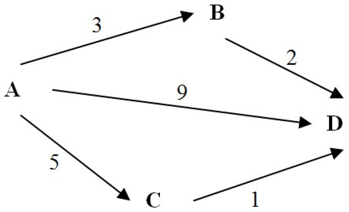
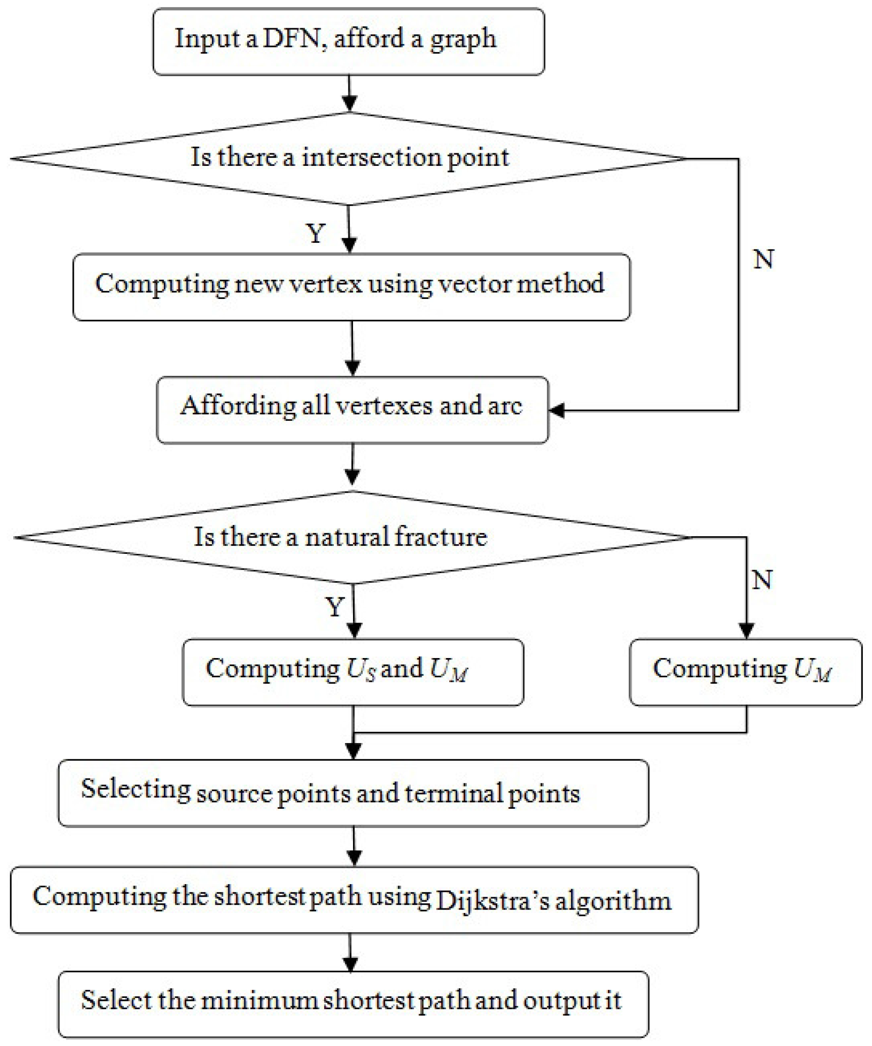
In this paper, a new method is presented to obtain the final configuration of fracture propagation with high computation efficiency, which combines Dijkstra’s algorithm, energy theory and vector method. Changes in hydraulic fracture propagation are generally attributed to various distribution properties of fractures (such as fracture length, fracture density and dip angle) and simulation conditions (like elastic modulus, normal stress pressure, Poisson’s ratio and so on). Hence, different parameters are analyzed, which can show how these parameters influence the propagation of hydraulic fracture. Some preliminaries are given in Section 2. Section 3 discusses how to obtain the configuration of propagated hydraulic fracture using Dijkstra’s Algorithm. Parameter analysis is done in Section 4. Section 5 states a discussion and some conclusions are given in Section 6.

2. Preliminaries

Graph $G(V,E)$ is a collection, which is composed of a vertex set $V\left(G\right)$ and edge set $E\left(G\right)$. In this paper, the element of $E\left(G\right)$ denotes fracture.

Definition 1. 

[12] Make $G=(V,E,W)$ be a weighted graph, where V is the vertex set, E is the edge set, and W is the weight matrix for E. W represents the cost from one vertex u to other vertex v (indicated by $\omega (u,v)$). If $e=(u,v)$, replace $\omega (u,v)$ with $\omega \left(e\right)$.

Definition 2. 

[12] The length of a path $p=(e_0,e_1,\dots ,e_k)$ is the sum of the weights of its constituent edges:

$$\begin{array}{c}\hfill length\left(P\right)=\sum _{i=1}^k\omega (e_{i-1},e_i).\end{array}$$

(1)

Definition 3. 

[12] The distance from u to v, shown as $\delta (u,v)$, is the shortest path with the minimum sum of the weights on the edges in a $u-v$ path. $u,v$ denoted start vertex and sink vertex, respectively.

The following example is given to illustrate the meaning of Definition 1–3, which is shown in Figure 2. Vertex A and D are the start vertex and terminal node, respectively. The weight value and shortest path can be obtained:

$$V=\{A,B,C,D\},$$

$$E=\left\{\omega \right(A,B)=3,\omega (A,D)=9,\omega (A,C)=5,\omega (B,D)=2,\omega (C,D)=1\}.$$

From Definition 2, it is easy to obtain that $length(A,D)=\omega (A,D)=9$ or $length(A,D)=\omega (A,B)+\omega (B,D)=5$. Hence, the distance from A to D is 5.

Dijkstra’s Algorithm

The shortest path problem can be divided into four situations in actual problems, and there are always four kinds of the corresponding algorithms [17]: (1) Dijkstra’s algorithm for Single Source Shortest Path, the weight of edge is non-negative [18]; (2) Bellman–Ford’s algorithm, it is also for the Single Source Shortest Path, and the weight of edge can be negative. However, the negative weight circuit cannot exist [19]; (3) Shortest Path Fastest Algorithm for Single Source Shortest Path—it is an improved algorithm based on the Bellman–Ford algorithm [20]; (4) Floyd algorithm for Shortest Path among all vertices—the weight of edge can be negative [21]. However, the negative weight circuit cannot be existed. For hydraulic fracturing, the weight of fracture is non-negative and the hydraulic fracture propagation belongs to the Single Source Shortest Path problem. Hence, Dijkstra’s algorithm is the most suitable method to simulate the hydraulic fracture during propagation of hydraulic fracturing.

Dijkstra’s algorithm can be used to find the shortest path between the node and every other [18]. Here, $V=\{v_0,v_1,v_2,\dots ,v_n\}$ is divided into two vertex sets: $S=\left\{v_0\right\}$ and $T=\{v_1,v_2,\dots ,v_n\}$ . Assume $v_0$ is the initial vertex, and $dist\left[v_i\right]$ is used to store the upper bound of the shortest path distance from $v_0$ to $v_i$. If the final shortest path from $v_0$ to $v_i$ is determined, denoted $S=S\cup v_i,$ $T=T\backslash v_i$. The algorithm repeatedly selects the node $v_i$ from T with the minimum $dist\left[v_i\right]$, and puts it in set S. The main steps for Dijkstra’s algorithm can be described as follows:

Step 1. Set $v_0$ is initial vertex,

$$\begin{array}{c}\hfill S\left[v_i\right]=\left\{\begin{array}{c}0,v_i\notin S\hfill \\ 1,v_i\in S\hfill \end{array}\right.\hspace{1em},\end{array}$$

and

$$\begin{array}{c}\hfill dist\left[v_i\right]=\left\{\begin{array}{c}{\omega }_{0i},i\ne 0\&(v_0,v_i)\in E\hfill \\ \infty ,(v_0,v_i)\notin E\hfill \\ 0,i=0\&(v_0,v_i)\in E\hfill \end{array}\right.\hspace{1em}i=1,2,\dots ,n.\end{array}$$

Step 2. Select the vertex $v_i$ in T, such that $dist\left[v_i\right]=\underset{v_j\in T}{min}dist\left[v_j\right]$. If $dist\left[v_i\right]=\infty$, stop, else go to Step 3.

Step 3. Set $S=S\cup v_i,T=T\backslash v_i$, and $S\left[v_i\right]=1$. If $T=\mathrm{⌀}$, stop, else go to Step 4.

Step 4. Update $dist\left[v_j\right]=min\{{\omega }_{0j},dist\left[v_i\right]+{\omega }_{ij}\}$. Go to Step 2.

An example is given to illustrate the working of the Dijsktra’s algorithm, which is shown in Figure 3. To begin with, the weight matrix should be computed. Assume that A is the start vertex, the weight of the minimum-weight paths from A to every other vertex is $+\infty$, and A to A is 0.

3. Model Description

In this section, Dijsktra’s algorithm is used to simulate the hydraulic fracture propagation in the DFN. DFN is given under the meter scale, which has two groups of fractures. During the hydraulic fracture propagation, two kinds of energies are used to describe different fracture propagation: mechanical energy and interface energy. The mechanical energy is used to keep natural fracture open, and interface energy is used to create new fractures. Combined the mechanical energy and interface energy, the fracture weighted formula is successfully deduced.

3.1. Discrete Fracture Network

An example of DFN is a two-dimensional horizontal section of a rock with 4 m length, 4 m width, which is shown in Figure 4. DFN is composed of two groups of random fractures, and the blue lines represent natural fractures. The fracture number is 250, the length of a fracture is 0.2 m. The angle between the two groups of fractures and the dip angle (which also means the angle between one set fractures to the maximum principal stress direction) is ${60}^{\circ }$. Figure 4 also shows that the DFN is not fully connected from one side to the other. During hydraulic fracturing, new fractures are the only way to link natural fractures. Therefore, new fractures should be an important factor in Dijsktra’s algorithm.

3.2. The Fracture Intersection Point

There are many fracture intersection points in Figure 4. During hydraulic fracturing, when fracture fluid flows through a fracture intersection, fracture fluid will enter into two fractures. Hence, the new vertices generated from fracture intersections have a significant influence on DFN connection, and these new vertices must be found out. Many mathematic methods to detect the fracture intersection have been studied, such as parameter equation and vector method [22]. Vector method is a great approach to this problem. $e_1=(u_1,v_1)$ and $e_2=(u_2,v_2)$ represent two fractures, respectively. Defining the two-dimensional vector cross product: $e_1\times e_2=u_1{v}_2-u_2{v}_1$. Vector quantities $r=(u_3,v_3)$ and $s=(u_4,v_4)$ represent the other two fractures, respectively. Supposing the two line segments run from $e_1$ to $e_1+r$ and from $e_2$ to $e_2+s$. The main steps are as follows [23]:

(1)

If $r\times s=0$ and $(e_2-e_1)\times r=0$, then the two lines are collinear. If either $0\le (e_2-e_1)•r\le r•r$ or $0\le (e_2-e_1)•s\le s•s$, then the two lines are overlapping.

(2)

If $r\times s=0$ and $(e_2-e_1)\times r=0$, but neither $0\le (e_2-e_1)•r\le r•r$ nor $0\le (e_2-e_1)•s\le s•s$, then the two lines are collinear but disjoint.

(3)

If $r\times s=0$ and $(e_2-e_1)\times r\ne 0$, then the two lines are parallel and non-intersecting.

(4)

If $r\times s=0$ and $0\le t,u\le 1$, the two line segments meet at the point $e_1+tr=e_2+us$.

(5)

Otherwise, the two line segments are not parallel but intersect.

Using this method, all of the fracture intersection points can be found in DFN, which are shown in Figure 5, and marked by the red points.

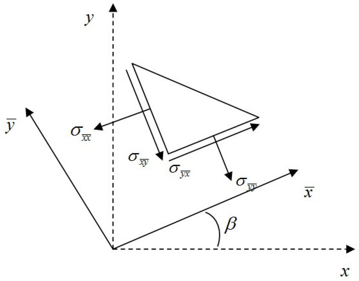
3.3. The Fracture Weighted Formula

During hydraulic fracturing, energy can well explain the fracture propagation, which includes the elastic modulus, normal stress, Poisson’s ratio and so on [1]. Hence, the fracture weighted formula with energy will be innovatively deduced in this section. Energy can be divided into two categories: mechanical energy and interface energy. The mechanical energy is for keeping natural fractures open, and it is related to the fracture length. Interface energy is for creating new fractures, which is related to the fracture length [24]. The energies during fracture propagation are described by weighted value in the shortest path problem. Considering fracture length, fracture type and so on, the weighted values of fracture are different from each other. Mechanical energy should be considered in natural fractures. However, for new fractures, both mechanical energy and interface energy should be considered during computing the weight values of new fractures [24]. The derivation processes of the fracture weighted formulas with energy are described as follows:

Assuming that fracture propagation length is c and the normal stress is P. The expression is [24]:

$$\begin{array}{c}\hfill P={\sigma }_{xx}{sin}^2\beta -2{\sigma }_{xy}sin\beta cos\beta +{\sigma }_{yy}{cos}^2\beta ,\end{array}$$

(2)

where $S[{\sigma }_{xx},{\sigma }_{xy},{\sigma }_{yy}]$ is in situ stress, and ${\sigma }_{xx}$ and ${\sigma }_{yy}$ are the x and y direction stress. ${\sigma }_{xy}$ is shear stress and β is the dip angle, and the schematic describing the fracture and stresses is shown in Figure 6.

Mechanical energy $U_M$ is the sum of the bearing system potential energy $U_A$ and elastic strain energy $U_E$ [25]:

$$\begin{array}{c}\hfill d{U}_M=d{U}_A+d{U}_E=-P^{2}d\lambda \left(c\right)+\frac{1}{2}{P}^{2}d\lambda \left(c\right)=-\frac{1}{2}{P}^{2}d\lambda \left(c\right),\end{array}$$

(3)

$$\begin{array}{c}\hfill G=-d{U}_M/dc=\frac{1}{2}{P}^{2}d\lambda \left(c\right)/dc,\end{array}$$

(4)

$$\begin{array}{c}\hfill \lambda \left(c\right)=\frac{2(1-\nu )}{G}·c,\end{array}$$

(5)

where G is the energy per unit area or length [25], c is the length of fracture, $\lambda \left(c\right)$ is elastic compliance, and ν is Poisson’s ratio. Generating Equations (4) and (5) into Equation (3), it is easy to obtain

$$\begin{array}{c}\hfill U_M=\frac{P^2{c}^2(1-\nu )}{G}.\end{array}$$

(6)

In another case, new fracture length is c, then, interface energy $U_S$ is:

$$\begin{array}{c}\hfill U_S=4·c·\gamma ,\end{array}$$

(7)

where γ is the surface energy per unit area or length.

During fracture propagation, the weighted value of natural fracture is computed only by considering mechanical energy $U_M$, which can be better understood by the energy of keeping the fractures open during gas extraction. The weighted value of new fractures is computed by combining mechanical energy $U_M$ and interface energy $U_S$.

4. Result of Numerical Modeling

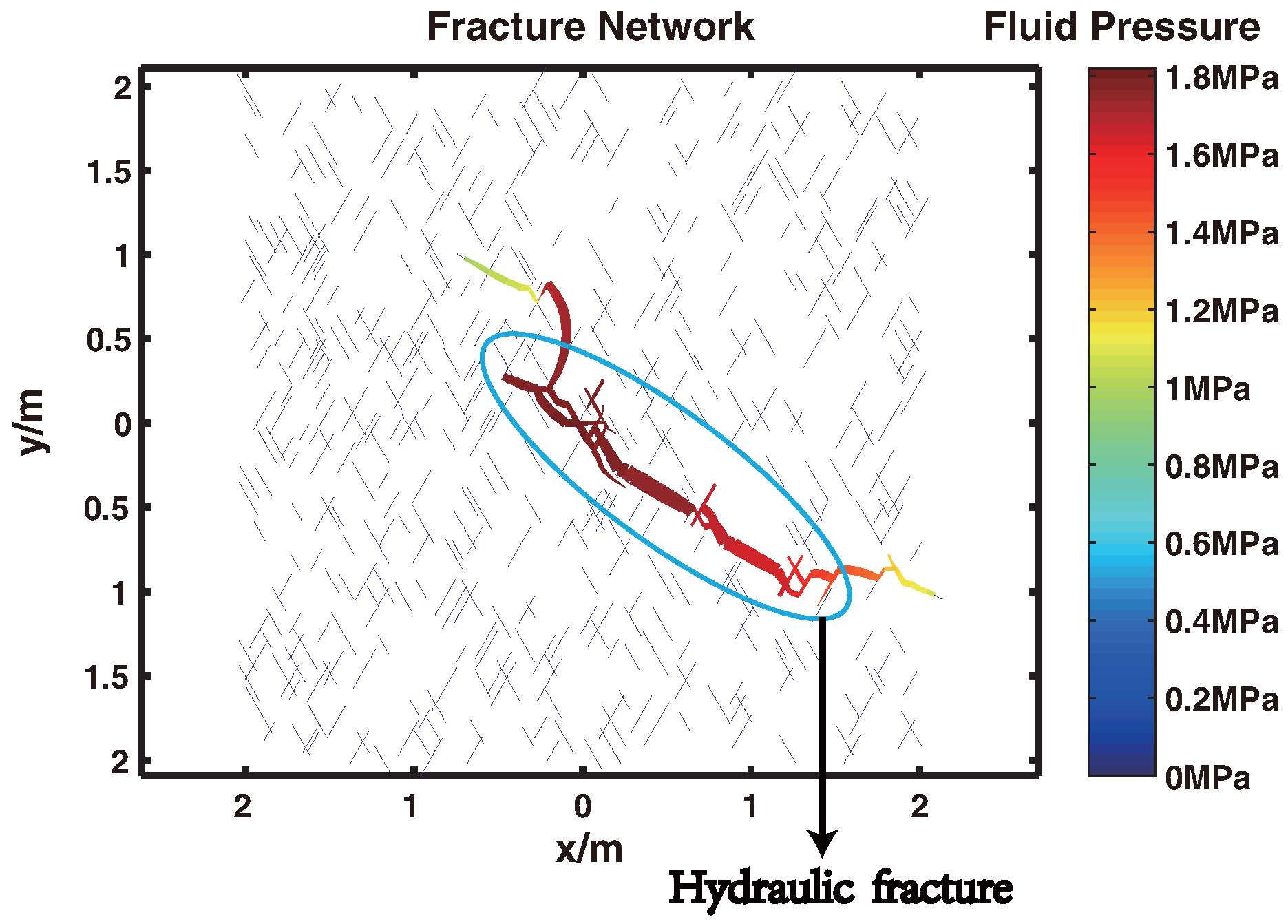
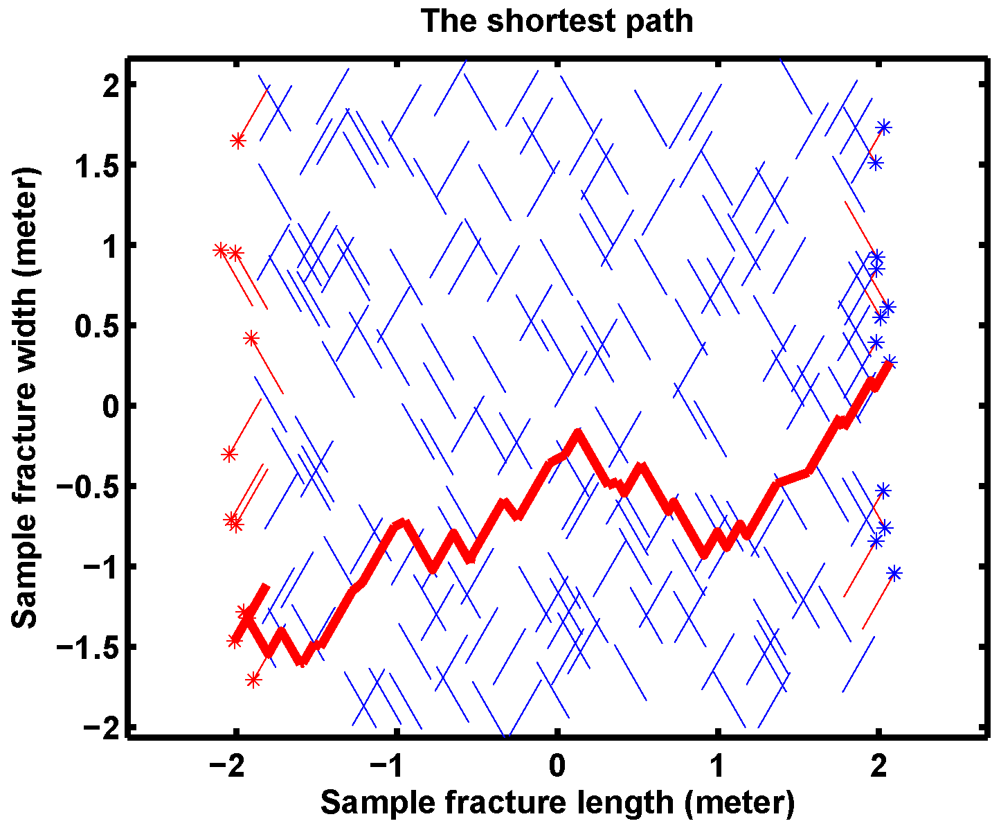
4.1. Determination of the Hydraulic Fracture

Assume that the direction of the maximum principal stress is horizontal. Predetermine that the new fracture in DFN has connected its downstream vertex with its upstream vertex. For example, vector $(u,v)$ represents the start vertex (indicated by $u(u_x,u_y)$) and the final point (indicated by $v(v_x,v_y)$) of a branch. If $u_x$ is greater than $v_x$, vertex u is marked as an upstream vertex. In addition, vertex v is made as a downstream vertex. On the contrary, vertex v is marked as upstream vertex. All the vertices in Figure 4 and intersections in Figure 5 are the elements of set V.

Select N vertices from the set V as source points. If the abscissa of these N vertices is smaller than other vertices’, these N vertices are denoted as initial vertices. In addition, found N vertices are also regarded as terminal points, if the abscissa of these N vertices are larger than other vertices’. Assume $N=12$. The initial vertices and terminal points can be obtained in this DFN by comparing their abscissa values, which are shown in Figure 7. The vertices marked by red ’*’ are the start vertices (indicated by $v_1,v_2,\dots ,v_{12}$), and the terminal points are marked by a blue ’*’ (indicated by $u_1,u_2,\dots ,u_{12}$).

Basing on Definition 3 of Section 2, the DFN is a collection of three sets, indicated by $G(V,E,W)$. All endpoints of the fracture in Figure 3 and intersection points in Figure 4 are the element of set $V=v_1,v_2,..,v_n$, where $v_{j+12}=u_j(j=1,2,\dots ,12)$, and $V_1=v_{2}5,v_{2}6,..,vn$ describe the intersection points. The element of set E is composed of the fracture in DFN. Set W is computed by Equations (6) and (7) in Section 3.3. Take in situ stress $S[{\sigma }_{xx},{\sigma }_{xy},{\sigma }_{yy}]=[6.0\times {10}^{7}Pa,1.0\times {10}^{7}Pa,5.0\times {10}^{7}Pa]$ in Equation (2), Poisson’s ratio $\nu =0.35$ in Equations (5) and (6), $\gamma =1.0\times {10}^{6}J/m$ in Equation (7). Based on Definition 2.2–2.3 in Section 2, $p_{ij}=(v_i,u_j)$ presents the weight from $v_i$ to $u_j$$(i,j=1,2,\dots ,12)$, and $\delta (u,v)$ represents the shortest path with the minimum sum of the fracture weights. Using Dijkstra’s algorithm with energy, the hydraulic fracture of DFN can be obtained. The main steps of algorithm are as follows:

Step 1. Set $x=1$.

Step 2. For the initial vertex $v_x$, initialize $S=\left\{v_x\right\},T=V\backslash S,dist\left[v_i\right]$ and $ver\left[x\right]$:

$$\begin{array}{c}\hfill S\left[v_i\right]=\left\{\begin{array}{c}0,v_i\notin S\hfill \\ 1,v_i\in S\hfill \end{array}\right.\hspace{1em},\end{array}$$

$$\begin{array}{c}\hfill dist\left[v_i\right]=\left\{\begin{array}{c}{U}_M,i\ne x\&(v_0,v_i)\in E\&naturefracture\hfill \\ U_M+U_S,i\ne x\&(v_0,v_i)\in E\&newfracture\hfill \\ \infty ,\left(v_{,}{v}_i\right)\notin E\hfill \\ 0,i=x\&(v_x,v_i)\in E\hfill \end{array}\right.\hspace{1em}i=1,2,\dots ,n,\end{array}$$

and

$$ver\left[x\right]=0,x=1,2,\dots ,12.$$

Step 3. Select the vertex $v_i$ in T, such that $dist\left[v_i\right]=\underset{v_j\in T}{min}dist\left[v_j\right]$. If $dist\left[v_i\right]=\infty$, stop, else go to Step 4.

Step 4. Set $S=S\cup v_i,T=T\backslash v_i$, and $S\left[v_i\right]=1$. If $T=\mathrm{⌀}$, stop, else go to Step 5.

Step 5. Update $dist\left[v_j\right]=min\{{\omega }_{0j},dist\left[v_i\right]+{\omega }_{ij}\}$. Go to Step 3.

Step 6. Find $p_{xj}$, and let $P_x=\underset{j=1,2,\dots ,12}{min}\left\{p_{xj}\right\}$.

Step 7. Set $ver\left[x\right]=1$, $x=x+1$ and go to Step 2 until $x=12$.

Step 8. $\delta (u,v)=\underset{j=1,2,\dots ,12}{min}\left\{P_j\right\}$.

In addition, the algorithm flow chart is shown in Figure 8. From the above steps, it can be shown that the potential distances are now recorded as updated edge weights so that no additional memory is required. Through combining the vector method and geological parameter with Dijkstra’s algorithm, the hydraulic fracture of DFN is obtained, which is marked by a red color in Figure 9.

4.2. Experiment and Comparison

The sample is sampled in the Jiaoshiba shale gas field, Sichuan Basin, and the sample’s detail is shown in Figure 10. We drilled a hole with diameter 10 mm and depth 50 mm in the center of sample. During the hydraulic fracturing test, the axial stress and confining stress are 30 MPa and 20 MPa, respectively, and the injection rate is 30 ml/min.

For comparison, the parameters in Section 4.1 are equal to the experimental conditions. The failure morphology of the sample after the experiment is shown in Figure 11a. It is worth noting that the sample has obvious horizontal bedding faces. The direction of natural fractures in the numerical model is along these horizontal bedding faces. As demonstrated in Figure 11a, it can be shown that the hydraulic fracture propagates through the whole sample along the direction of maximum horizontal in situ stress. Figure 11b shows the simulation results using the method above in Section 4.1. It can be shown that the hydraulic fracture, obtained by the method in this paper, is similar to the the failure morphology of the sample.

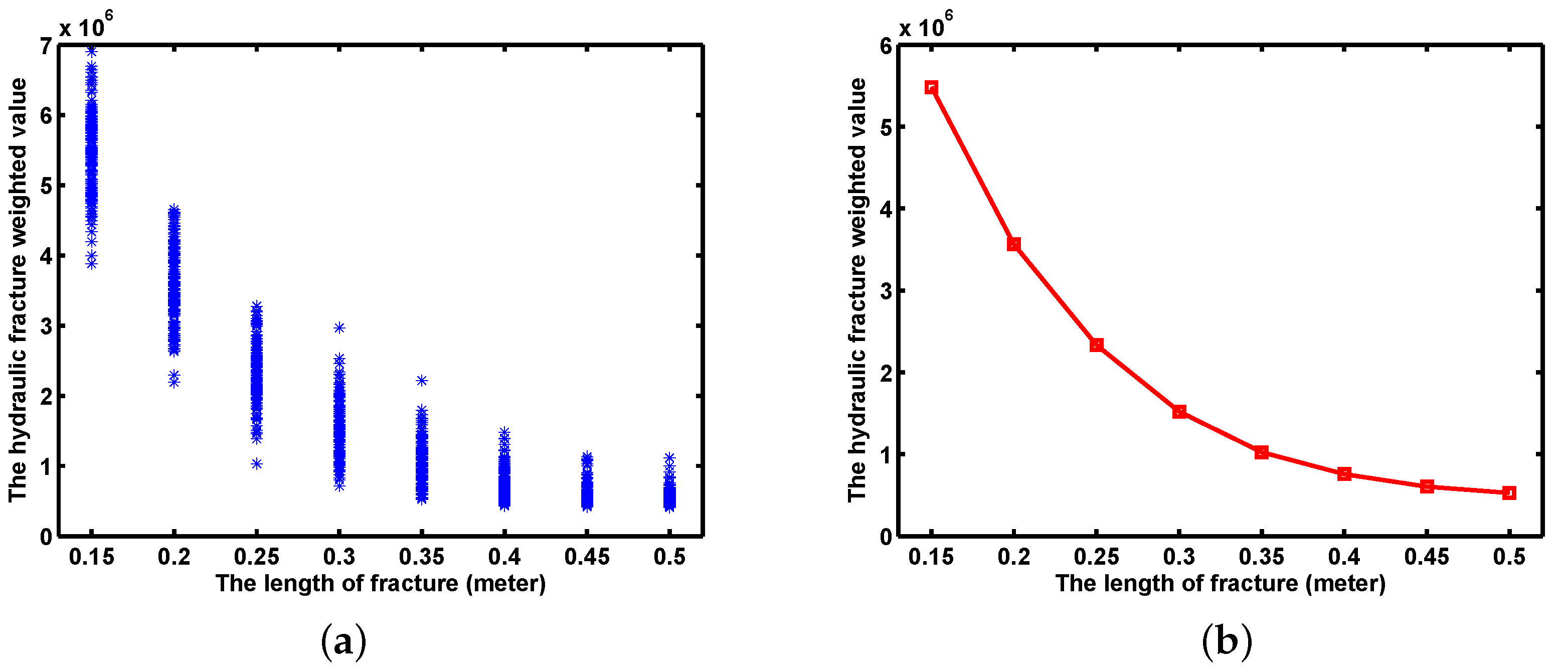
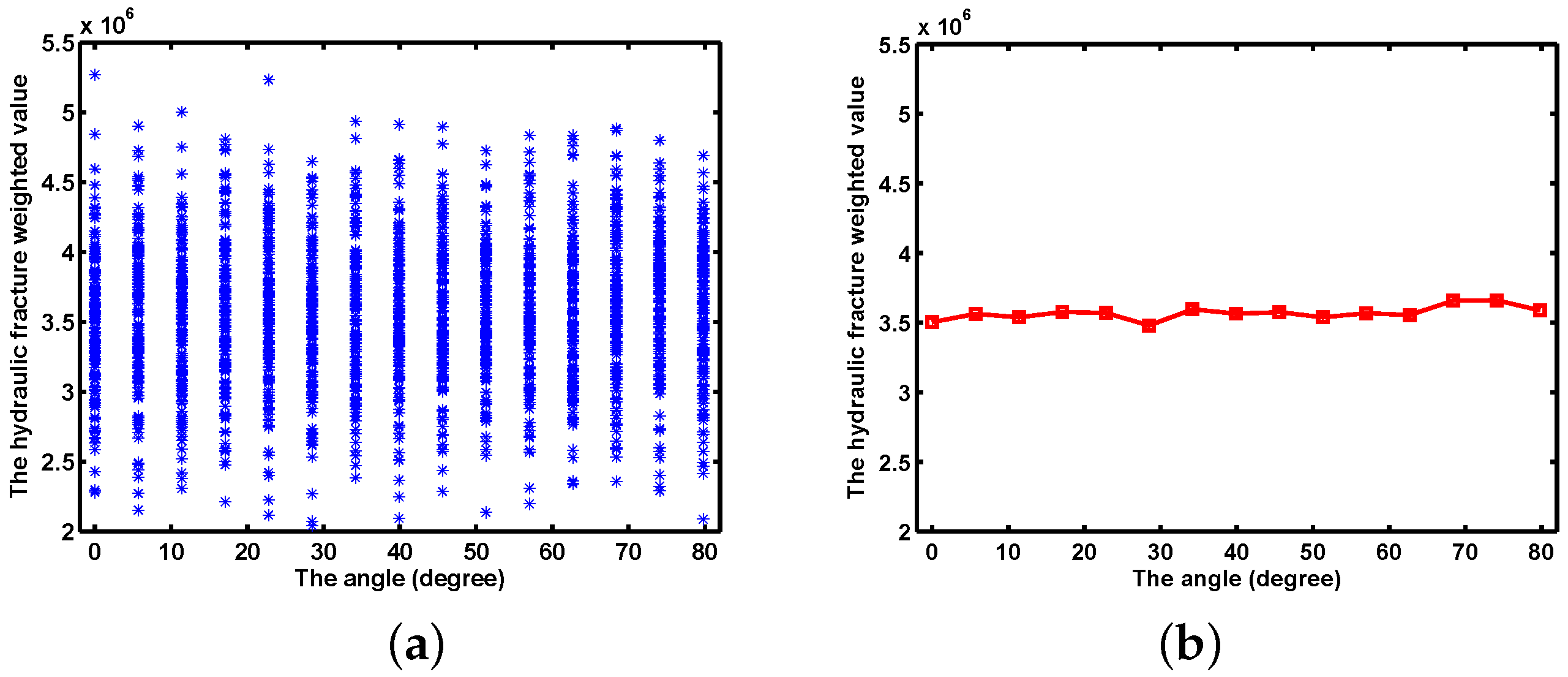
4.3. Parameter Sensitivity Analysis

During fracture propagation, several factors can influence the propagation of hydraulic fracture in a discrete fracture network system, such as intensity of discrete fracture (fracture number, and marked with n), fracture length (marked with l), and dip angle (marked with α). In this section, the weighted value of hydraulic fracture is used to explore how these parameters influence the hydraulic fracture propagation. Here, the DFN is a two-dimensional horizontal section of a rock with 4 m length and 4 m width. Assuming that the DFN is static, partially connected and randomly distributed. The maximum principal stress direction keeps in line with the x-axis, and many groups of fractures are repeated computing for eliminating the influence of randomness. Figure 12, Figure 13, Figure 14 and Figure 15 show quantitative comparison of the behavior of the models based on different parameters.

Firstly, the influence of fracture number on the weight value of hydraulic fracture is shown in Figure 12. The trends of scatter distribution and average distribution are consistent with each other, and the weight value of hydraulic fracture decreases with the increasing of fracture number. That also means that the greater the fracture, the better for the hydraulic fracture propagation. Then, Figure 13 shows that the weight value of hydraulic fracture decreases with increasing of fracture length. It also indicates that as the fracture length is growing, the weight value of the hydraulic fracture is reducing. Longer fracture length will benefit the hydraulic fracture propagation. Finally, as demonstrated in Figure 14, it has little influence on the weight value of hydraulic fracture for different values of α when the angle between two groups of fracture keeps orthogonal. Hence, the influence of different values of α on the weight value of hydraulic fracture will also be studied under two groups of fractures are not orthogonal. Figure 15 shows the weight value of the hydraulic fracture firstly decreases and then increases with the increase of α when the angle between two groups of fractures are ${20}^{\circ }$. That being said, the farther away from the maximum stress direction, the larger the weight value of the hydraulic fracture.

5. Discussion

The operating parameters are effective only when the geological parameters are favorable for fracturing treatment. Therefore, the evaluation of the geological parameters before hydraulic fracturing is crucial to hydraulic fracturing treatment in shale formation. The effects of geological parameters are investigated, including fracture density, fracture length, and dip angle (the angle between one group of fracture and the maximum principal stress direction). By analyzing the sensitivity of DFN with various parameters, it can be concluded that the hydraulic fracture weight value decreases with increase in the intensity of fracture and fracture length, and increases with increasing of the angle between fractures to the maximum principal stress direction. It means that the fracture density and fracture length are significant to the DFN connectivity.

6. Conclusions

Increases in natural gas extraction are being driven by rising energy demands, mandates for cleaner burning fuels, and the economics of energy use [26]. Directional drilling and hydraulic fracturing technologies are allowing expanded natural gas extraction from organic-rich shales [27], while the propagation of the hydraulic fracture is the crux of hydraulic fracturing, and can provide a high-conductivity path for methane migration in the low permeability reservoir. Accompanying the benefits of such extraction [28] are public concerns about hydraulic fracturing that are ubiquitous but lack a strong scientific foundation. In this paper, Dijkstra’s algorithm, energy theory and vector methods were combined to simulate the hydraulic fracture propagation in DFN during hydraulic fracturing. We successfully give the shortest path weighted value formula of fracture propagation, and obtained the hydraulic fracture in DFN during hydraulic fracturing. The direction of the hydraulic fracture is also simulated, which plays a key role in identifying the spatial position of the well bore during hydraulic fracturing. Numerical results with experimental data show that the hydraulic fracture obtained by our method is similar to the failure morphology of the sample (see Figure 11).

This study has played a very important role in the hydraulic fracturing field, including the following aspects: (1) obtaining the extension direction of the fracture; through comparing the energies of fracture propagation in different directions, the direction of the minimum energy fracture propagation is the most likely direction of the hydraulic fracture; (2) evaluating the complexity of the DFN. Through Dijkstra’s algorithm, several paths can be obtained whose energies are smaller. If the positions of these paths are very near, it is shown that the hydraulic fracture is a great advantage and it is harder to get a complex fracture network. On the contrary, if the positions of these paths are very far away, it is shown that the hydraulic fracture lacks strength and it is easy to get a complex fracture network; and (3) through computing the weight value of hydraulic fracture, the injected energy during hydraulic fracturing can be obtained, which is strongly related with pore pressure and fluid viscosity. During hydraulic fracturing treatment, the pore pressure decreases with the distance far away from the well bore, and this factor has been considered while computing fracture weight value.

References

- Veatch, R.W., Jr.; Moschovidis, Z.A.; Fast, C.R. An Overview of Hydraulic Fracturing, Recent Advances in Hydraulic Fracturing; Gidley, J.L., Holditch, S.A., Nierode, D.E., Veatch, R.W., Jr., Eds.; Society of Petroleum Engineers, Henry L Doherty Series Monograph: Beijing, China, 1986; Volume 12. [Google Scholar]
- Zhang, Z.; Li, X.; He, J.; Wu, Y.; Zhang, B. Numerical Analysis on the Stability of Hydraulic Fracture Propagation. Energies 2015, 8, 9860–9877. [Google Scholar] [CrossRef]
- Weng, X.W. Modeling of complex hydraulic fractures in naturally fractured formation. J. Unconv. Oil Gas Resour. 2015, 9, 114–135. [Google Scholar] [CrossRef]
- McClure, M.; Horne, R. Characterizing Hydraulic Fracturing with a Tendency-for-Shear-Stimulation Test. SPE Reserv. Eval. Eng. 2014, 11, 233–243. [Google Scholar] [CrossRef]
- Kresse, O.; Weng, X.W.; Gu, H.R. Numerical Modeling of Hydraulic Fractures Interaction in Complex Naturally Fractured Formations. Rock Mech. Rock Eng. 2013, 46, 555–568. [Google Scholar] [CrossRef]
- Mohammadnejad, T.; Khoei, A.R. An extended finite element method for hydraulic fracture propagation in deformable porous media with the cohesive crack model. Finite Elem. Anal. Design 2013, 73, 77–95. [Google Scholar] [CrossRef]
- Ferté, G.; Massina, P.; Moësba, N. 3D crack propagation with cohesive elements in the extended finite element method. Comput. Methods Appl. Mech. Eng. 2016, 300, 347–374. [Google Scholar]
- Fu, P.; Johnson, S.M.; Carrigan, C. An explicitly coupled hydro-geomechanical model for simulating hydraulic fracturing in complex discrete fracture networks. Int. J. Numer. Anal. Methods Geomech. 2012, 37, 2278–2300. [Google Scholar] [CrossRef]
- Verde, A.; Ghassemi, A. Modeling injection/extraction in a fracture network with mechanically interacting fractures using an efficient displacement discontinuity method. Int. J. Rock Mech. Min. Sci. 2015, 77, 278–286. [Google Scholar] [CrossRef]
- Dong, C.Y.; De Pater, C.J. Numerical implementation of displacement discontinuity method and its application in hydraulic fracturing. Comput. Methods Appl. Mech. Eng. 2001, 191, 745–760. [Google Scholar] [CrossRef]
- Behnia, M.; Goshtasbi, K.; Fatehi Marji, M.; Golshani, A. On the crack propagation modeling of hydraulic fracturing by a hybridized displacement discontinuity/boundary collocation method. J. Min. Environ. 2012, 2, 1–16. [Google Scholar]
- Bello, I.; Britton, J.R.; Kaul, A. Topics in Contemporary Mathematics. Chapter 15 (Graph Theory), 9th ed.; Richard Stratton: New York, NY, USA, 2008. [Google Scholar]
- Cherkassky, B.V.; Goldberg, A.V.; Radzik, T. Shortest paths algorithms: Theory and experimental evaluation. Math. Program. 1996, 73, 129–174. [Google Scholar] [CrossRef]
- Shirinivas, S.G.; Vetrivel, S.; Elango, N.M. Applications of graph theory in computer science an overview. Int. J. Eng. Sci. Technol. 2012, 2, 4610–4621. [Google Scholar]
- Klampfer, S.; Mohrko, J.; Cucej, Z.; Chowdhury, A. Graph’s theory approach for searching the shortest routing path in RIP protocol: A case study. Przeglad Elektrotech. 2012, 8, 224–231. [Google Scholar]
- Sarbu, I.; Valea, E.S. Application of operational research to determine optimal path for a water transmission main. In Proceedings of the International MultiConference of Engineers and Computer Scientists, Hong Kong, China, 13–15 March 2013.
- Falcao, A.X.; Stolfi, J.; de Alencar Lotufo, R. The image foresting transform: Theory, algorithms, and applications. IEEE Trans. Pattern Anal. Mach. Intell. 2004, 26, 19–29. [Google Scholar] [CrossRef] [PubMed]
- Lu, X.; Camitz, M. Finding the shortest paths by node combination. Appl. Math. Comput. 2011, 217, 6401–6408. [Google Scholar] [CrossRef]
- Zhang, W.; Chen, H.; Jiang, C.; Zhu, L. Improvement And Experimental Evaluation Bellman–Ford Algorithm. In 2013 International Conference on Advanced ICT and Education (ICAICTE-13); Atlantis Press: Paris, France, 2013. [Google Scholar]
- Garcia-Luna-Aceves, J.J. A minimum-hop routing algorithm based on distributed information. Comput. Netw. ISDN Syst. 1989, 16, 367–382. [Google Scholar] [CrossRef]
- Hougardy, S. The Floyd-Warshall algorithm on graphs with negative cycles. Inf. Process. Lett. 2010, 110, 279–281. [Google Scholar] [CrossRef]
- Snyder, V.; Sisam, C.H. Analytic Geometry Of Space. In Merchant Books; University of Michigan Library: Michigan, MI, USA, 2007. [Google Scholar]
- Stack Overflow. Available online: http://stackoverflow.com/questions/563198/how-do-you-detect-where-two-line-segments-intersect (accessed on 18 February 2009).
- McClure, M.; Horne, R.N. Discrete Fracture Network Modeling of Hydraulic Stimulation: Coupling Flow and Geomechanics; Springer Science & Business Media: London, UK, 2013. [Google Scholar]
- Lawn, B. Fracture of Brittle Solods; Cambridge University Press: Cambridge, UK, 1993. [Google Scholar]
- Nehring, D. Natural gas from shale bursts onto the scene. Science 2010, 328, 1624–1626. [Google Scholar]
- Osborn, S.G.; Vengosh, A.; Warner, N.R.; Jackson, R.B. Methane contamination of drinking water accompanying gas-well drilling and hydraulic fracturing. Proc. Natl. Acad. Sci. USA 2011, 108, 8172–8176. [Google Scholar] [CrossRef] [PubMed]
- Kargbo, D.M.; Wilhelm, R.G.; Campbell, D.J. Natural gas plays in the Marcellus shale: Challenges and potential opportunities. Environ. Sci. Technol. 2010, 44, 5679–5684. [Google Scholar] [CrossRef] [PubMed]
© 2016 by the authors; licensee MDPI, Basel, Switzerland. This article is an open access article distributed under the terms and conditions of the Creative Commons Attribution (CC-BY) license (http://creativecommons.org/licenses/by/4.0/).
Share and Cite
Wu, Y.; Li, X. Numerical Simulation of the Propagation of Hydraulic and Natural Fracture Using Dijkstra’s Algorithm. Energies 2016, 9, 519. https://doi.org/10.3390/en9070519
Wu Y, Li X. Numerical Simulation of the Propagation of Hydraulic and Natural Fracture Using Dijkstra’s Algorithm. Energies. 2016; 9(7):519. https://doi.org/10.3390/en9070519
Chicago/Turabian StyleWu, Yanfang, and Xiao Li. 2016. "Numerical Simulation of the Propagation of Hydraulic and Natural Fracture Using Dijkstra’s Algorithm" Energies 9, no. 7: 519. https://doi.org/10.3390/en9070519