On Real-Time Fault Detection in Wind Turbines: Sensor Selection Algorithm and Detection Time Reduction Analysis

Abstract

In this paper, we address the problem of real-time fault detection in wind turbines. Starting from a data-driven fault detection method, the contribution of this paper is twofold. First, a sensor selection algorithm is proposed with the goal to reduce the computational effort of the fault detection method. Second, an analysis is performed to reduce the data acquisition time needed by the fault detection method, that is, with the goal of reducing the fault detection time. The proposed methods are tested in a benchmark wind turbine where different actuator and sensor failures are simulated. The results demonstrate the performance and effectiveness of the proposed algorithms that dramatically reduce the number of sensors and the fault detection time.

1. Introduction

Wind energy, in contrast to burning fossil fuels, is a clean and inexhaustible renewable energy source. It is on the way to becoming a leading electricity generating technology in Europe. There is now 142 GW of installed wind power capacity with 131 GW onshore and 11 GW offshore [1]. Wind turbines have become the largest rotating machines on earth, while plans for future turbines show even larger diameters up to 200 m (10 to 15 MW) and there is a need for research to cope with the many challenges the technology upscaling implies [2]. One of the key challenges is to make wind energy one of the most cost-efficient energy sources. Avoiding unexpected failures seems to be the crux of the matter because of the impact on downtime and thus on the cost of energy [3]. Continuous monitoring of wind turbine health using automated failure detection algorithms can improve turbine reliability and reduce maintenance costs by detecting failures before they reach a catastrophic stage and by eliminating unnecessary scheduled maintenance.

Nowadays, a tremendous amount of information is available to support operation of wind turbines. Through the use of lidars, wind data become available, upstream as well as within the turbines. All turbines permanently collect big data from hundreds of sensors, ranging from gearbox oil temperature to stresses in the blade root. All control actions use sensor data as inputs, with increasing resolution and complexity. Condition monitoring relies on clever processing of these data. Proper selection and reduction of the amount of the data is of the utmost importance [3].

Traditionally, condition monitoring systems for wind turbines have focused on the detection of failures in the main bearing, generator, and gearbox, some of the highest cost components on a wind turbine. Two widely-used methods are vibration analysis and oil monitoring [4]. These are standalone systems that require installation of sensors and hardware. In this paper, the fault detection strategy presented in [5] is used. It uses on-line SCADA (supervisory control and data acquisition) data already available at an industrial wind turbine to provide advance warning of failures.

In this work, first, sensor selection is investigated based on principal components analysis. The goal is to select a reduced number of sensors to be used by the fault detection method. From a practical point of view, a reduced number of sensors installed in the wind turbine leads to a reduced cost of installation and maintenance. In addition, from a computational point of view, less sensors implies less computational effort. Due to these practical issues (reduction of hardware costs, possibility of storage or physical space, computational and communication burden), sensor selection is currently being studied and applied to several research areas. For instance, Chepuri and Leus [6] propose convex relaxations techniques to select the best subset of sensors that guarantees some recommended performance. Similarly, Bai et al. [7] suggest a sensor selection schedule to minimize the observation cost on a sequential probability ratio test (SPRT). With respect to a more precise problem, Miao et al. [8] investigated the performance of combinations of several metal-oxide sensors for the discrimination of a set of ginsengs. Equivalently and yet in the field of wind turbines, Wang et al. [9] review and apply standard techniques proposed by Jolliffe [10] for the sensor selection for wind turbine condition monitoring.

The contribution of this paper is twofold. On one hand, a sensor selection algorithm based on principal component analysis (PCA) is used to select the sensors that best separate the healthy and the faulty wind turbine with the purpose of fault detection thus leading to some reduction in the computational and communication effort. On the other hand, a reduction in the data acquisition time needed by the fault detection method is investigated. In this second case, the goal is to reduce the fault detection time.

In order to test the proposed sensor selection algorithm as well as the fault detection time reduction, we used data from simulations using the comprehensive wind turbine simulator FAST (fatigue, aerodynamic, structures and turbulence) for a 5 MW wind turbine [11]. Different actuator and sensor failures are simulated following the benchmark model proposed in [12]. In this benchmark challenge, a more sophisticated wind turbine model (using FAST) and updated fault scenarios are presented. This higher-fidelity model also allows the use of more realistic wind inputs that vary spatially across the rotor plane in addition to temporally.

This paper is organized as follows. In Section 2, the reference wind turbine, wind model, as well as generator-converter actuator and pitch actuator models are recalled. The fault scenarios are described in Section 3. Next, in Section 4, the proposed sensor selection algorithm is presented as well as results showing the effect on the fault detection strategy when using the reduced number of sensors. Thereafter, in Section 5, an analysis is performed to reduce the number of time instants needed by the fault detection method, thus reducing the fault detection time. Then, Section 6 analyzes the effect on the performance of the fault detection strategy when a reduced number of sensors is used altogether with reducing the fault detection time. Finally, conclusions are drawn in Section 7.

2. Reference WT

The National Renewable Energy Laboratory (NREL) offshore 5-MW baseline wind turbine [13] is used in the simulations. This model is used as a reference by research teams throughout the world to standardize baseline offshore wind turbine specifications and to quantify the benefits of advanced land- and sea-based wind energy technologies. In this work, the wind turbine is operated in its onshore version and in the above-rated wind-speed range. The main properties of this turbine are listed in

Table 1. Gross properties of the wind turbine [13].

Reference Wind Turbine
Rated power	5 MW
Number of blades	3
Rotor/Hub diameter	126 m, 3 m
Hub Height	90 m
Cut-In, Rated, Cut-Out Wind Speed	3 m/s, 11.4 m/s, 25 m/s
Rated generator speed	1173.7 rpm
Gearbox ratio	97

.

In this work, the proposed fault detection method is SCADA-data based, that is, it uses data already collected at the wind turbine controller. In particular,

Table 2. Assumed available measurements. These sensors are representative of the types of sensors that are available on a MW-scale commercial wind turbine.

Number	Sensor Type	Symbol	Units
1	Generated electrical power	$P_{e,m}$	kW
2	Rotor speed	${\omega }_{r,m}$	rad/s
3	Generator speed	${\omega }_{g,m}$	rad/s
4	Generator torque	${\tau }_{c,m}$	Nm
5	first pitch angle	${\beta }_{1,m}$	deg
6	second pitch angle	${\beta }_{2,m}$	deg
7	third pitch angle	${\beta }_{3,m}$	deg
8	fore-aft acceleration at tower bottom	$a_{fa,m}^b$	m/s2
9	side-to-side acceleration at tower bottom	$a_{ss,m}^b$	m/s2
10	fore-aft acceleration at mid-tower	$a_{fa,m}^m$	m/s2
11	side-to-side acceleration at mid-tower	$a_{ss,m}^m$	m/s2
12	fore-aft acceleration at tower top	$a_{fa,m}^t$	m/s2
13	side-to-side acceleration at tower top	$a_{ss,m}^t$	m/s2

presents assumed available data on a MW-scale commercial wind turbine that is used in this work by the fault detection method.

The reference wind turbine has a conventional variable-speed, variable blade-pitch-to-feather configuration. In such wind turbines, the conventional approach for controlling power-production operation relies on the design of two basic control systems: a generator-torque controller and a rotor-collective blade-pitch controller. In this work, the baseline torque and pitch controllers are utilized, but the generator-converter and the pitch actuators are modeled and implemented externally; i.e., apart from the embedded FAST code. This will facilitate to model different type of faults on the generator and the pitch actuator. The next subsections recall these models and also the wind model used to generate the wind data.

2.1. Wind Modeling

The TurbSim stochastic inflow turbulence tool (National Wind Technology Center, Boulder, CO, USA) [14] has been used. It provides the ability to drive design code (e.g., FAST) simulations of advanced turbine designs with simulated inflow turbulence environments that incorporate many of the important fluid dynamic features known to adversely affect turbine aeroelastic response and loading.

The generated wind data has the following characteristics: Kaimal turbulence model with intensity set to $10\%$, logarithmic profile wind type, mean speed is set to $18.2$ m/s and simulated at hub height, and the roughness factor is set to $0.01$ m.

In this work, every simulation is ran with a different wind data set.

2.2. Generator-Converter Actuator Model and Pitch Actuator Model

The generator-converter and the pitch actuators are modeled apart from the embedded FAST code, with the objective to ease the model of different type of faults on these parts of the wind turbine.

On one hand, the generator-converter can be modeled by a first-order differential system [12]:

$${\displaystyle \frac{{\tau }_r\left(s\right)}{{\tau }_c\left(s\right)}=\frac{{\alpha }_{gc}}{s+{\alpha }_{gc}}}$$

where ${\tau }_r$ and ${\tau }_c$ are the real generator torque and its reference (given by the controller), respectively, and we set ${\alpha }_{gc}=50$ [13]. The power produced by the generator, $P_e\left(t\right)$, can be modeled by [12]:

$$P_e\left(t\right)={\eta }_g{\omega }_g\left(t\right){\tau }_r\left(t\right)$$

where ${\eta }_g$ is the efficiency of the generator and ${\omega }_g$ is the generator speed. In the numerical experiments, ${\eta }_g=0.98$ is used [12].

On the other hand, the three pitch actuators are modeled as a second-order linear differential equation, pitch angle ${\beta }_i\left(t\right)$, and its reference $u\left(t\right)$ (given by the collective-pitch controller) [12]:

$${\displaystyle \frac{{\beta }_i\left(s\right)}{u\left(s\right)}=\frac{{\omega }_n^2}{s^2+2\xi {\omega }_{n}s+{\omega }_n^2},i=1,2,3}$$

(1)

where ${\omega }_n$ and ξ are the natural frequency and the damping ratio, respectively. In the fault free case, these values are set to ${\omega }_n=11.11$ rad/s, and $\xi =0.6$.

3. Fault Description

In this paper, the different faults proposed in the fault tolerant control benchmark [15] will be considered, as gathered in

Table 3. Fault scenarios.

Fault	Type	Description
1	Pitch actuator	Change in dynamics: high air content in oil (${\omega }_n=5.73$ rad/s, $\xi =0.45$)
2	Pitch actuator	Change in dynamics: pump wear (${\omega }_n=7.27$ rad/s, $\xi =0.75$)
3	Pitch actuator	Change in dynamics: hydraulic leakage (${\omega }_n=3.42$ rad/s, $\xi =0.9$)
4	Generator speed sensor	Scaling (gain factor equal to $1.2$)
5	Pitch angle sensor	Stuck (fixed value equal to 5 deg)
6	Pitch angle sensor	Stuck (fixed value equal to 10 deg)
7	Pitch angle sensor	Scaling (gain factor equal to $1.2$)
8	Torque actuator	Offset (offset value equal to 2000 Nm)

. These faults selected by the benchmark cover different parts of the wind turbine, different fault types and classes, and different levels of severity.

Usually, pitch systems use either an electric or a fluid power actuator. However, the fluid power subsystem has lower failure rates and better capability of handling extreme loads than the electrical systems. Therefore, fluid power pitch systems are preferred on multi-MW size and offshore turbines. However, general issues such as leakage, contamination, component malfunction and electrical faults make current systems work sub-optimal [16]. In this work, faults in the pitch actuator are considered in the hydraulic system, which result in changed dynamics due to either a high air content in oil (fault 1) or a drop in pressure in the hydraulic supply system due to pump wear (fault 2) or hydraulic leakage (fault 3) [17], as well as pitch position sensor faults (faults 5–7).

Pump wear (fault 2) is an irreversible slow process over the years that results in low pump pressure. As this wear is irreversible, the only possibility to fix it is to replace the pump, which will happen after pump wear reaches certain level. Meanwhile, the pump will still be operating and the system dynamics is slowly changing, while the turbine structure should be able to withstand the effects of this fault. Pump wear after approximately 20 years of operation might result in pressure reduction to $75\%$ of the rated pressure, which is reflected by the faulty natural frequency ${\omega }_n=7.27$ rad/s and a fault damping ratio of $\xi =0.75$.

Hydraulic leakage (fault 3) is another irreversible incipient fault but is introduced considerably faster than the pump wear. Leakage of pitch cylinders can be internal or external [16]. When this fault reaches a certain level, system repair is necessary, and if the leakage is too fast (normally due to external leakage), it will lead to a pressure drop and the preventive procedure is deployed to shut down the turbine before the blade is stuck in undesired position (if the hydraulic pressure is too low, the hydraulic system will not be able to move the blades that will cause the actuator to be stuck in its current position resulting in blade seize). The fast pressure drop is easy to detect (even visually as it is normally related to external leakage) and requires immediate reaction; however, the slow hydraulic leakage reduces the dynamics of the pitch system, and for a reduction of $50\%$ of the nominal pressure the natural frequency under this fault condition is reduced to ${\omega }_n=3.42$ rad/s and the corresponding damping ratio is $\xi =0.9$. In this work, the slow (internal) hydraulic leakage is studied.

On the contrary to pump wear and hydraulic leakage, high air content in the oil (fault 1) is an incipient reversible process, which means that the air content in the oil may disappear without any necessary repair to the system. The nominal value of the air content in the oil is $7\%$, whereas the high air content in the oil corresponds to $15\%$. The effect of such a fault is expressed by the new natural frequency ${\omega }_n=5.73$ rad/s and the damping ratio of $\xi =0.45$ (corresponding to the high air content in the oil).

The generator speed measurement is done using encoders. The gain factor fault (fault 4) is introduced when the encoder reads more marks on the rotating part than actually present, which can happen as a result of dirt or other false markings on the rotating part.

Faults in the pitch position measurement (pitch position sensor fault) are also advised. This is one of the most important failure modes found on actual systems [16,18]. The origin of these faults is either electrical or mechanical, and it can result in either a fixed value (faults 5 and 6) or a changed gain factor (fault 7) on the measurements. In particular, the fixed value fault should be easy to detect, and, therefore, it is important that a fault detection, isolation, and accommodation scheme be able to deal with this fault. If not handled correctly, these faults will influence the pitch reference position because the pitch controller is based on these pitch position measurements.

Finally, a converter torque offset fault is considered (fault 8). It is difficult to detect this fault internally (by the electronics of the converter controller). However, from a wind turbine level, it is possible to be detected, isolated, and accommodated because it changes the torque balance in the wind turbine power train.

4. Sensor Selection

The goal of this section is to present a method to select a reduced number of sensors to be used in the fault detection method. Classical approaches to sensor or variable selection may be summarized in the following example. Let us assume that we have N sensors or variables that are measuring during $(L-1)\Delta$ seconds, where Δ is the sampling time and $L\in \mathbb{N}$. The discretized measures of each sensor can be arranged as a column vector ${\mathbf{x}}^i={(x_1^i,x_2^i,\dots ,x_L^i)}^T,i=1,\dots ,N$ so we can build up a $L\times N$ matrix as follows:

$$\begin{array}{c}\hfill X=\left({\mathbf{x}}^1\left|{\mathbf{x}}^2\right|\cdots |{\mathbf{x}}^N\right)=\left(\begin{array}{cccc}{x}_1^1& x_1^2& \cdots & x_1^N\\ x_2^1& x_2^2& \cdots & x_2^N\\ ⋮& ⋮& \ddots & ⋮\\ x_i^1& x_i^2& \cdots & x_i^N\\ ⋮& ⋮& \ddots & ⋮\\ x_L^1& x_L^2& \cdots & x_L^N\end{array}\right)\in {\mathcal{M}}_{L\times N}\left(\mathbb{R}\right)\end{array}$$

(2)

It is worth noting that each column in matrix X in Equation (2) represents the measures of a single sensor or variable. In general, when some application of principal component analysis is used, and when a large number of variables or sensors is available, the results are usually slightly changed if just a subset of the sensors is used [10]. Consequently, a simple approach is to calculate the subset of σ sensors that maximizes the multiple correlation of the $N-\sigma$ non-selected sensors with respect to the σ selected sensors. A similar approach, based on principal component analysis (PCA), that is also used in the field of feature extraction, is to compute the first principal components and observe the coefficients of the corresponding eigenvectors. More precisely, if the unit eigenvector related to the largest eigenvalue is

$$\begin{array}{c}\hfill u_1={\alpha }_1{s}_1+{\alpha }_2{s}_2+\cdots +{\alpha }_N{s}_N,\sum _{i=1}^N{\alpha }_i^2=1\end{array}$$

the sensor associated with the smallest coefficient $\alpha =\underset{i=1,\dots ,N}{min}{\alpha }_i$ can be neglected. A comprehensive list of methods for deciding on which variables or sensors to reject can be found in [10].

However, when multiway principal component analysis is applied to data coming from N sensors at L discretization instants and n experimental trials, the information can be stored in an unfolded $n\times (N\times L)$ matrix as follows:

$$\mathbf{X}=\left(\begin{array}{ccccccccccc}{x}_{11}^1& x_{12}^1& \cdots & x_{1L}^1& x_{11}^2& \cdots & x_{1L}^2& \cdots & x_{11}^N& \cdots & x_{1L}^N\\ ⋮& ⋮& \ddots & ⋮& ⋮& \ddots & ⋮& \ddots & ⋮& \ddots & ⋮\\ x_{i1}^1& x_{i2}^1& \cdots & x_{iL}^1& x_{i1}^2& \cdots & x_{iL}^2& \cdots & x_{i1}^N& \cdots & x_{iL}^N\\ ⋮& ⋮& \ddots & ⋮& ⋮& \ddots & ⋮& \ddots & ⋮& \ddots & ⋮\\ x_{n1}^1& x_{n2}^1& \cdots & x_{nL}^1& x_{n1}^2& \cdots & x_{nL}^2& \cdots & x_{n1}^N& \cdots & x_{nL}^N\end{array}\right)$$

(3)

In this case, a column in matrix $\mathbf{X}$ in Equation (3) no longer represents the values of a variable at different time instants but the measurements of a variable at one particular time instant in the whole set of experimental trials. Consequently, even though PCA can be applied to these kind of matrices as a way to reduce the dimensionality of the data and to create a new coordinates space where the data is best represented, the eigenvalues and eigenvectors of the covariance matrix ${\mathbf{C}}_{\mathbf{X}}=\frac{1}{N\times L-1}{\mathbf{X}}^T\mathbf{X}$ cannot be directly used to infer what variables or sensors could be neglected. In addition, we are not only interested in the sensors that best model the healthy wind turbine but the sensors that best discriminate the faulty wind turbine. This is one of the main differences between the work proposed by Wang et al. [9] and the strategy presented in the present work: while in [9] the authors use principal component analysis to reduce the number of inputs (sensors) to build the model of the active and reactive powers of a wind turbine as a multiple-input multiple-output linear system, in this paper, PCA is used to find the sensors that best separate the healthy and the faulty wind turbine with the purpose of fault detection.

The overall strategy to select the best subset of sensors that discriminate the healthy and the faulty wind turbine is to create a multiway PCA model measuring a healthy wind turbine. With the model, and for each fault scenario, we measure the Euclidean distance between the arithmetic mean of the projections into the PCA model that come from the healthy wind turbine and the mean of the projections that come from the faulty one. The subset of sensors related to the maximum distance between the means of each pair of projections will be the selected sensors. The detailed algorithmic procedure is described in the next subsection.

4.1. Sensor Selection Algorithm

Sensor selection can be essentially viewed as a combinatorial problem involving some kind of performance criterion over all possible options. In the subsequent algorithm, some parameters must be selected, such as the cardinal of the initial set of variables or sensors N, the number of sensors σ to be combined or the number ℓ of principal components:

• Consider a set $\mathcal{S}=\{s_1,s_2,\dots ,s_{13}\}$ of $N=13$ sensors as in Table 2.
• Consider a number of sensors σ to be combined, $\sigma =2,\dots ,N$.
• Consider the set ${\Omega }^{\sigma }=\left\{{\mathcal{S}}_1^{\sigma },{\mathcal{S}}_2^{\sigma },\dots ,{\mathcal{S}}_{(\genfrac{}{}{0pt}{}{N}{\sigma })}^{\sigma }\right\}$ formed by the $(\genfrac{}{}{0pt}{}{N}{\sigma })$ $\sigma$-subsets of σ elements out of the set $\mathcal{S}$. For instance, ${\mathcal{S}}_1^2=\{s_1,s_2\}$. In a general case, we will write ${\mathcal{S}}_k^{\sigma }=\{s_{\left(1\right)},s_{\left(2\right)},\dots ,s_{\left(\sigma \right)}\}$, $k=1,\dots ,(\genfrac{}{}{0pt}{}{N}{\sigma })$, where $s_{\left(1\right)}$ refers to the first sensor in ${\mathcal{S}}_k^{\sigma }$, $s_{\left(2\right)}$ to the second sensor in the set and so on.
• For each $\sigma$-subset ${\mathcal{S}}_k^{\sigma }\in {\Omega }^{\sigma },k=1,\dots ,(\genfrac{}{}{0pt}{}{N}{\sigma })$, measure, from a healthy wind turbine, sensors $s_{\left(1\right)},s_{\left(2\right)},\dots ,s_{\left(\sigma \right)}$ during $(nL-1)\Delta$ seconds.
• Arrange the collected data coming from the σ sensors in a matrix $\mathbf{X}\in {\mathcal{M}}_{n\times (\sigma \times L)}\left(\mathbb{R}\right)$ as follows:

  $$\mathbf{X}=\left(\begin{array}{ccccccccccc}{x}_{11}^{\left(1\right)}& x_{12}^{\left(1\right)}& \cdots & x_{1L}^{\left(1\right)}& x_{11}^{\left(2\right)}& \cdots & x_{1L}^{\left(2\right)}& \cdots & x_{11}^{\left(\sigma \right)}& \cdots & x_{1L}^{\left(\sigma \right)}\\ ⋮& ⋮& \ddots & ⋮& ⋮& \ddots & ⋮& \ddots & ⋮& \ddots & ⋮\\ x_{i1}^{\left(1\right)}& x_{i2}^{\left(1\right)}& \cdots & x_{iL}^{\left(1\right)}& x_{i1}^{\left(2\right)}& \cdots & x_{iL}^{\left(2\right)}& \cdots & x_{i1}^{\left(\sigma \right)}& \cdots & x_{iL}^{\left(\sigma \right)}\\ ⋮& ⋮& \ddots & ⋮& ⋮& \ddots & ⋮& \ddots & ⋮& \ddots & ⋮\\ x_{n1}^{\left(1\right)}& x_{n2}^{\left(1\right)}& \cdots & x_{nL}^{\left(1\right)}& x_{n1}^{\left(2\right)}& \cdots & x_{nL}^{\left(2\right)}& \cdots & x_{n1}^{\left(\sigma \right)}& \cdots & x_{nL}^{\left(\sigma \right)}\end{array}\right)$$

  (4)
• Choose a number ℓ of principal components, $\ell =1,\dots ,\sigma \times L$.
• Perform a sensor-based group scaling and find the PCA model $\mathbf{P}\in {\mathcal{M}}_{(\sigma \times L)\times (\sigma \times L)}\left(\mathbb{R}\right)$ (also called loading matrix) as detailed in [5, Section 3.1]. Consider the reduced matrix $\widehat{\mathbf{P}}:=\mathbf{P}(:,1:\ell )\in {\mathcal{M}}_{(\sigma \times L)\times \ell }\left(\mathbb{R}\right)$ related to the ℓ highest eigenvalues, formed by the first ℓ columns of matrix $\mathbf{P}$.
• Measure, from a healthy wind turbine, sensors $s_{\left(1\right)},s_{\left(2\right)},\dots ,s_{\left(\sigma \right)}$ during $(n_{\text{h}}L-1)\Delta$ seconds. Arrange the collected data coming from the σ sensors in a matrix ${\mathbf{Y}}_{\text{h}}\in {\mathcal{M}}_{n_{\text{h}}\times (\sigma \times L)}\left(\mathbb{R}\right)$ as follows:

  $${\mathbf{Y}}_{\text{h}}=\left(\begin{array}{ccccccccccc}{y}_{11}^{\left(1\right)}& y_{12}^{\left(1\right)}& \cdots & y_{1L}^{\left(1\right)}& y_{11}^{\left(2\right)}& \cdots & y_{1L}^{\left(2\right)}& \cdots & y_{11}^{\left(\sigma \right)}& \cdots & y_{1L}^{\left(\sigma \right)}\\ ⋮& ⋮& \ddots & ⋮& ⋮& \ddots & ⋮& \ddots & ⋮& \ddots & ⋮\\ y_{i1}^{\left(1\right)}& y_{i2}^{\left(1\right)}& \cdots & y_{iL}^{\left(1\right)}& y_{i1}^{\left(2\right)}& \cdots & y_{iL}^{\left(2\right)}& \cdots & y_{i1}^{\left(\sigma \right)}& \cdots & y_{iL}^{\left(\sigma \right)}\\ ⋮& ⋮& \ddots & ⋮& ⋮& \ddots & ⋮& \ddots & ⋮& \ddots & ⋮\\ y_{n_{\text{h}}1}^{\left(1\right)}& y_{n_{\text{h}}2}^{\left(1\right)}& \cdots & y_{n_{\text{h}}L}^{\left(1\right)}& y_{n_{\text{h}}1}^{\left(2\right)}& \cdots & y_{n_{\text{h}}L}^{\left(2\right)}& \cdots & y_{n_{\text{h}}1}^{\left(\sigma \right)}& \cdots & y_{n_{\text{h}}L}^{\left(\sigma \right)}\end{array}\right)$$

  (5)

  Perform a sensor-based group scaling and project the data to the principal component space using the matrix product ${\widehat{\mathbf{T}}}_{\text{h}}={\mathbf{Y}}_{\text{h}}\widehat{\mathbf{P}}\in {\mathcal{M}}_{n_{\text{h}}\times \ell }\left(\mathbb{R}\right)$. Define $t_{\text{h}}^i\in {\mathbb{R}}^{\ell },i=1,\dots ,n_{\text{h}}$ each row vector of matrix ${\widehat{\mathbf{T}}}_{\text{h}}$. Note that $n_{\text{h}}$ is a natural number not necessarily equal to n in Step 4.
• Measure, from a faulty wind turbine, sensors $s_{\left(1\right)},s_{\left(2\right)},\dots ,s_{\left(\sigma \right)}$ during $(n_{\text{f}}L-1)\Delta$ seconds. Arrange the collected data coming from the σ sensors in a matrix ${\mathbf{Y}}_{\text{f}}\in {\mathcal{M}}_{n_{\text{f}}\times (\sigma \times L)}\left(\mathbb{R}\right)$ as follows:

  $${\mathbf{Y}}_{\text{f}}=\left(\begin{array}{ccccccccccc}{z}_{11}^{\left(1\right)}& z_{12}^{\left(1\right)}& \cdots & z_{1L}^{\left(1\right)}& z_{11}^{\left(2\right)}& \cdots & z_{1L}^{\left(2\right)}& \cdots & z_{11}^{\left(\sigma \right)}& \cdots & z_{1L}^{\left(\sigma \right)}\\ ⋮& ⋮& \ddots & ⋮& ⋮& \ddots & ⋮& \ddots & ⋮& \ddots & ⋮\\ z_{i1}^{\left(1\right)}& z_{i2}^{\left(1\right)}& \cdots & z_{iL}^{\left(1\right)}& z_{i1}^{\left(2\right)}& \cdots & z_{iL}^{\left(2\right)}& \cdots & z_{i1}^{\left(\sigma \right)}& \cdots & z_{iL}^{\left(\sigma \right)}\\ ⋮& ⋮& \ddots & ⋮& ⋮& \ddots & ⋮& \ddots & ⋮& \ddots & ⋮\\ z_{n_{\text{f}}1}^{\left(1\right)}& z_{n_{\text{f}}2}^{\left(1\right)}& \cdots & z_{n_{\text{f}}L}^{\left(1\right)}& z_{n_{\text{f}}1}^{\left(2\right)}& \cdots & z_{n_{\text{f}}L}^{\left(2\right)}& \cdots & z_{n_{\text{f}}1}^{\left(\sigma \right)}& \cdots & z_{n_{\text{f}}L}^{\left(\sigma \right)}\end{array}\right)$$

  (6)

  Perform a sensor-based group scaling and project the data to the principal component space using the matrix product ${\widehat{\mathbf{T}}}_{\text{f}}={\mathbf{Y}}_{\text{f}}\widehat{\mathbf{P}}\in {\mathcal{M}}_{n_{\text{f}}\times \ell }\left(\mathbb{R}\right)$. Define $t_{\text{f}}^i\in {\mathbb{R}}^{\ell },i=1,\dots ,n_{\text{f}}$ each row vector of matrix ${\widehat{\mathbf{T}}}_{\text{f}}$. Note again that $n_{\text{f}}$ is a natural number not necessarily equal to n in Step 4 neither $n_{\text{h}}$ in Step 8.
• Define ${\mathit{\mu }}_{\text{h}}$ as the mean vector value of $t_{\text{h}}^i\in {\mathbb{R}}^{\ell },i=1,\dots ,n_{\text{h}}$, that is,

  $$\begin{array}{c}\hfill {\mathit{\mu }}_{\text{h}}=\frac{1}{n_{\text{h}}}\sum _{i=1}^{n_{\text{h}}}{t}_{\text{h}}^i\in {\mathbb{R}}^{\ell }\end{array}$$
• Define ${\mathit{\mu }}_{\text{f}}$ as the mean vector value of $t_{\text{f}}^i\in {\mathbb{R}}^{\ell },i=1,\dots ,n_{\text{f}}$, that is,

  $$\begin{array}{c}\hfill {\mathit{\mu }}_{\text{f}}=\frac{1}{n_{\text{f}}}\sum _{i=1}^{n_{\text{f}}}{t}_{\text{f}}^i\in {\mathbb{R}}^{\ell }\end{array}$$
• Compute the Euclidean norm $\parallel {\mathit{\mu }}_{\mathbf{\text{h}}}-{\mathit{\mu }}_{\mathrm{f}}{\parallel }_2=:{\mathcal{N}}_k^{\sigma }$ associated to the $\sigma$-subset ${\mathcal{S}}_k^{\sigma }\in {\Omega }^{\sigma }$, $k=1,\dots ,(\genfrac{}{}{0pt}{}{N}{\sigma })$.
• Find ${\kappa }^{\sigma }\in \left\{1,\dots ,(\genfrac{}{}{0pt}{}{N}{\sigma })\right\}$ where

  $$\begin{array}{c}\hfill {\mathcal{N}}_{{\kappa }^{\sigma }}^{\sigma }=\underset{k=1,\dots ,(\genfrac{}{}{0pt}{}{N}{\sigma })}{max}{\mathcal{N}}_k^{\sigma }\end{array}$$

  Therefore, given a particular fault scenario, the σ sensors in the set ${\mathcal{S}}_{{\kappa }^{\sigma }}^{\sigma }$ are the sensors that separate most of the data coming from the healthy wind turbine and the data coming from the faulty one.

4.2. Results of the Sensor Selection

The results of the sensor selection are summarized in

Table 4. Results of the sensor selection when the number of sensors to be combined is $\sigma =6$ for each of the eight fault scenarios described in Table 3.

	Sensors
Fault no.	1	2	3	4	5	6	7	8	9	10	11	12	13
1					✓	✓	✓		✓		✓		✓
2					✓	✓	✓		✓		✓		✓
3					✓	✓	✓		✓		✓		✓
4	✓	✓	✓		✓	✓	✓
5	✓	✓			✓	✓	✓						✓
6	✓		✓		✓	✓	✓						✓
7					✓	✓	✓		✓		✓		✓
8	✓				✓	✓	✓				✓		✓

when the number of sensors to be combined is $\sigma =6$ and the number of principal components is $\ell =10$.

More precisely, with respect to Table 4, it is worth noting that sensors 5, 6 and 7—corresponding to the first, second and third pitch angles—appear as selected in all of the eight fault scenarios. In this case, the sextuple of sensors is completed in fault scenarios 1, 2, 3 and 7 with sensors 9, 11 and 13 (side-to-side accelerations at tower bottom, mid-tower and tower top, respectively); in fault scenario 4 with sensors 1, 2 and 3 (generated electrical power, rotor speed and generator speed, respectively); in fault scenario 5 with sensors 1, 2 and 13 (generated electrical power, rotor speed and side-to-side acceleration at tower top, respectively); in fault scenario 6 with sensors 1, 3 and 13 (generated electrical power, generator speed and side-to-side acceleration at tower top, respectively); and finally, in fault scenario 8 with sensors 1, 11 and 13 (generated electrical power, side-to-side acceleration at mid-tower and tower top, respectively). From a physical point of view, when using $\sigma =6$ sensors, it is interesting to note that the three pitch angles and the side-to-side accelerations (and not the fore-aft accelerations that are in the same direction as the wind speed) are the most important signals to detect faults.

4.3. Fault Detection with a Reduced Number of Sensors

To analyze the effect on the overall performance of the fault detection strategy with a reduced number of sensors, we will study a total of 24 samples of $\nu =50$ elements each, corresponding to the following distribution:

• 16 samples of a healthy wind turbine, and
• Eight samples of a faulty wind turbine with respect to each of the eight particular fault scenarios defined in Table 3.

In this section, we will consider the following combination of $\sigma =6$ sensors:

• sensors $1,2,4,5,6$ and 7, that is, we will measure and collect the information provided by the generated electrical power, rotor speed, generator torque and the first, second and third pitch angles.

For this combination of sensors, each sample of $\nu =50$ elements is formed by the measures gathered from the sensors during $(\nu \times L-1)\Delta =312.4875$ seconds, where $L=500$ and the sampling rate $1/\Delta =80$ Hz. The fault detection strategy is based on the work by Pozo and Vidal [5], where multiway principal component analysis (MPCA) is first applied and then the so-called Welch–Satterthwaite method [19] to test for the equality of means. One of the key issues of the strategy presented in [5] is the way the data is collected and arranged in a matrix. To create the baseline pattern or PCA model, we measure the $\sigma =6$ sensors from a healthy wind turbine and all the collected data is organized in a matrix $\mathbf{X}\in {\mathcal{M}}_{n\times (N\times L)}$ as follows:

$$\begin{array}{cc}\hfill \mathbf{X}& =\left(\begin{array}{ccccccccccc}{x}_{11}^{\left(1\right)}& x_{12}^{\left(1\right)}& \cdots & x_{1L}^{\left(1\right)}& x_{11}^{\left(2\right)}& \cdots & x_{1L}^{\left(2\right)}& \cdots & x_{11}^{\left(\sigma \right)}& \cdots & x_{1L}^{\left(\sigma \right)}\\ ⋮& ⋮& \ddots & ⋮& ⋮& \ddots & ⋮& \ddots & ⋮& \ddots & ⋮\\ x_{i1}^{\left(1\right)}& x_{i2}^{\left(1\right)}& \cdots & x_{iL}^{\left(1\right)}& x_{i1}^{\left(2\right)}& \cdots & x_{iL}^{\left(2\right)}& \cdots & x_{i1}^{\left(\sigma \right)}& \cdots & x_{iL}^{\left(\sigma \right)}\\ ⋮& ⋮& \ddots & ⋮& ⋮& \ddots & ⋮& \ddots & ⋮& \ddots & ⋮\\ x_{n1}^{\left(1\right)}& x_{n2}^{\left(1\right)}& \cdots & x_{nL}^{\left(1\right)}& x_{n1}^{\left(2\right)}& \cdots & x_{nL}^{\left(2\right)}& \cdots & x_{n1}^{\left(\sigma \right)}& \cdots & x_{nL}^{\left(\sigma \right)}\end{array}\right)\hfill \\ & =\left({\mathbf{X}}^{\left(1\right)}\left|{\mathbf{X}}^{\left(2\right)}\right|\cdots |{\mathbf{X}}^{\left(\sigma \right)}\right)\hfill \end{array}$$

(7)

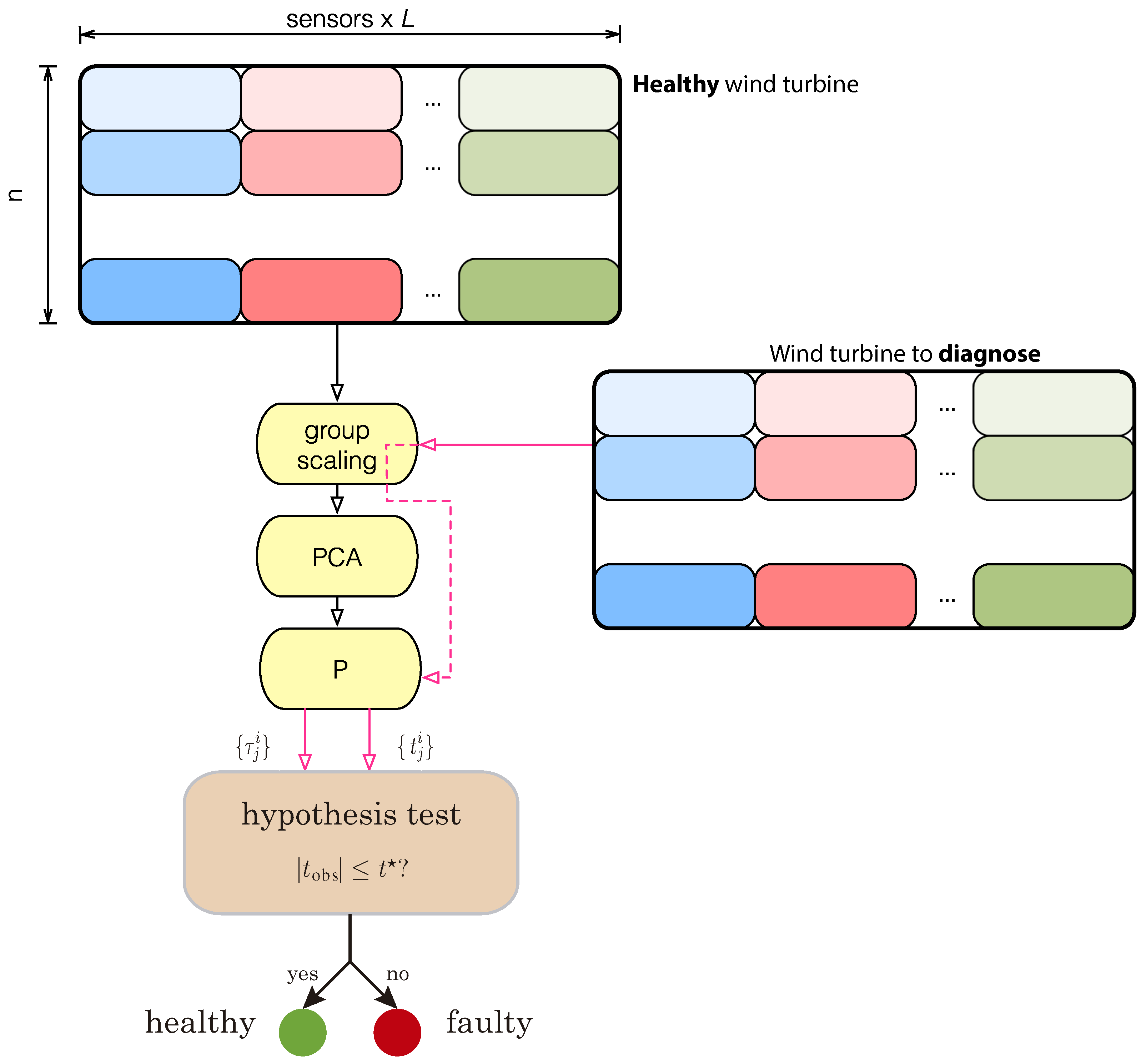
where the superindex $s=1,\dots ,\sigma$ of each element $x_{ij}^{\left(s\right)},i=1,\dots ,n,j=1,\dots ,L$ in the matrix represents the number of sensors. For the sake of completeness, we summarize in the following itemized list the fault detection strategy presented in [5], which is also illustrated in Figure 1:

• Sensor group-scaling is applied to matrix $\mathbf{X}$ in Equation (7) so the mean of each column is 0 and the standard deviation of each sensor submatrix ${\mathbf{X}}^{\left(s\right)},s=1,\dots ,\sigma$ is 1.
• The covariance matrix ${\mathbf{C}}_{\mathbf{X}}$ is computed according to the expression

  $$\begin{array}{c}\hfill {\mathbf{C}}_{\mathbf{X}}=\frac{1}{n-1}{\mathbf{X}}^T\mathbf{X}\in {\mathcal{M}}_{(\sigma \times L)\times (\sigma \times L)}\left(\mathbb{R}\right)\end{array}$$
• The eigenvalues and eigenvectors of matrix ${\mathbf{C}}_{\mathbf{X}}$ are computed. The eigenvectors (principal components) constitute the columns of the transformation matrix $\mathbf{P}$—also called PCA model or baseline pattern— according to the eigenvalues in descending order.
• With respect to the first principal component, for instance, the baseline sample is defined as the set of numbers $\left\{{\tau }_1^i\right\}:=\mathbf{X}(i,:)\times \mathbf{P}\times {\mathbf{e}}_1,i=1,\dots ,n$, where ${\mathbf{e}}_1$ is the first vector of the canonical basis.
• When the measures of the $\sigma =6$ sensors are obtained from the current wind turbine to be diagnosed, a new matrix Y has to be constructed as in Equation (7):

  $$\begin{array}{cc}\hfill \mathbf{Y}& =\left(\begin{array}{ccccccccccc}{y}_{11}^{\left(1\right)}& y_{12}^{\left(1\right)}& \cdots & y_{1L}^{\left(1\right)}& y_{11}^{\left(2\right)}& \cdots & y_{1L}^{\left(2\right)}& \cdots & y_{11}^{\left(\sigma \right)}& \cdots & y_{1L}^{\left(\sigma \right)}\\ ⋮& ⋮& \ddots & ⋮& ⋮& \ddots & ⋮& \ddots & ⋮& \ddots & ⋮\\ y_{i1}^{\left(1\right)}& y_{i2}^{\left(1\right)}& \cdots & y_{iL}^{\left(1\right)}& y_{i1}^{\left(2\right)}& \cdots & y_{iL}^{\left(2\right)}& \cdots & y_{i1}^{\left(\sigma \right)}& \cdots & y_{iL}^{\left(\sigma \right)}\\ ⋮& ⋮& \ddots & ⋮& ⋮& \ddots & ⋮& \ddots & ⋮& \ddots & ⋮\\ y_{\nu 1}^{\left(1\right)}& y_{\nu 2}^{\left(1\right)}& \cdots & y_{\nu L}^{\left(1\right)}& y_{\nu 1}^{\left(2\right)}& \cdots & y_{\nu L}^{\left(2\right)}& \cdots & y_{\nu 1}^{\left(\sigma \right)}& \cdots & y_{\nu L}^{\left(\sigma \right)}\end{array}\right)\hfill \\ & =\left({\mathbf{Y}}^{\left(1\right)}\left|{\mathbf{Y}}^{\left(2\right)}\right|\cdots |{\mathbf{Y}}^{\left(\sigma \right)}\right)\hfill \end{array}$$

  (8)

  Note that the number ν of rows in matrix $\mathbf{Y}$ in Equation (8) is a natural number not necessarily equal to the number of rows n in matrix $\mathbf{X}$ in Equation (7).
• Matrix $\mathbf{Y}$ in Equation (8) is scaled with respect to matrix $\mathbf{X}$ in Equation (7), that is, we subtract to the κ-th column of matrix $\mathbf{Y}$, $\kappa =1,\dots ,\nu \times L\times \sigma$, the mean of the κ-th column of matrix $\mathbf{X}$. Likewise, each element in the submatrix ${\mathbf{Y}}^{\left(s\right)},s=1,\dots ,\sigma$, is divided by the standard deviation of the submatrix ${\mathbf{X}}^{\left(s\right)}$.
• With respect to the first principal component, for instance, the sample of the current wind turbine to be diagnosed is defined as the set of numbers $\left\{t_1^i\right\}:=\mathbf{Y}(i,:)\times \mathbf{P}\times {\mathbf{e}}_1,i=1,\dots ,\nu$.
• The Welch–Satterthwaite test for the equality of means [19] is used with samples $\left\{{\tau }_1^i\right\}$ and $\left\{t_1^i\right\}$ to classify the current wind turbine to be diagnosed as healthy or not.

As stated before, a particular configuration of $\sigma =6$ sensors has been considered.

Table 5. Scheme for the presentation of the results in Table 6.

	Healthy Sample (H0)	Faulty Sample (H1)
Fail to reject $H_0$	Correct decision	Type II error (missing fault)
Reject $H_0$	Type I error (false alarm)	Correct decision

summarizes how the results in

Table 6. Categorization of the samples with respect to the presence or absence of a fault and the result of the test for each of the four scores when the size of the samples to diagnose is $\nu =50$ and the sensors used are numbers $1,2,4,5,6$ and 7.

	Score 1		Score 2		Score 3		Score 4
	H0	H1	H0	H1	H0	H1	H0	H1
Fail to reject $H_0$	16	0	8	1	9	0	13	1
Reject $H_0$	0	8	8	7	7	8	3	7

are organized. More precisely, Table 6 includes—using the measures of sensors $1,2,4,5,6$ and 7—the number of samples of the healthy wind turbine correctly classified by the test as healthy (correct decision); the number of samples of the faulty wind turbine correctly classified as faulty (correct decision); the number of samples of the faulty wind turbine wrongly classified as healthy (type II error or missing fault); and the number of samples of the healthy wind turbine wrongly classified as faulty (type I error or false alarm). It is worth noting that, for this configuration, type I errors (false alarms) and type II errors (missing faults) occur when we consider scores 2, 3 or 4, i.e., when the test is based purely on the first score all the classifications are accurate.

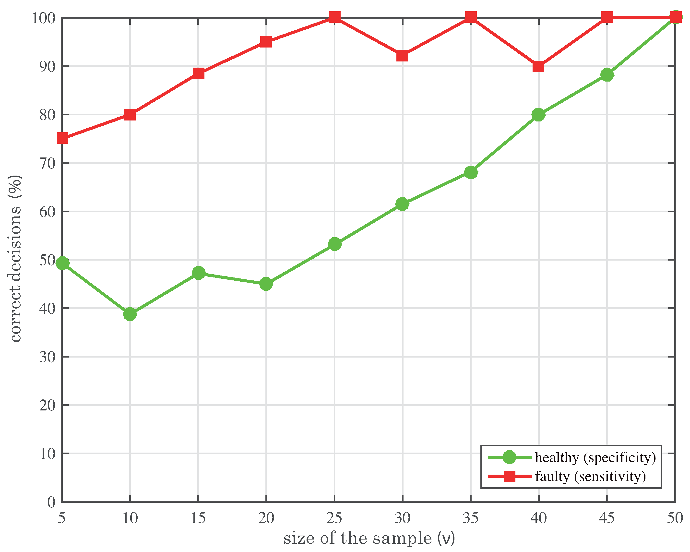
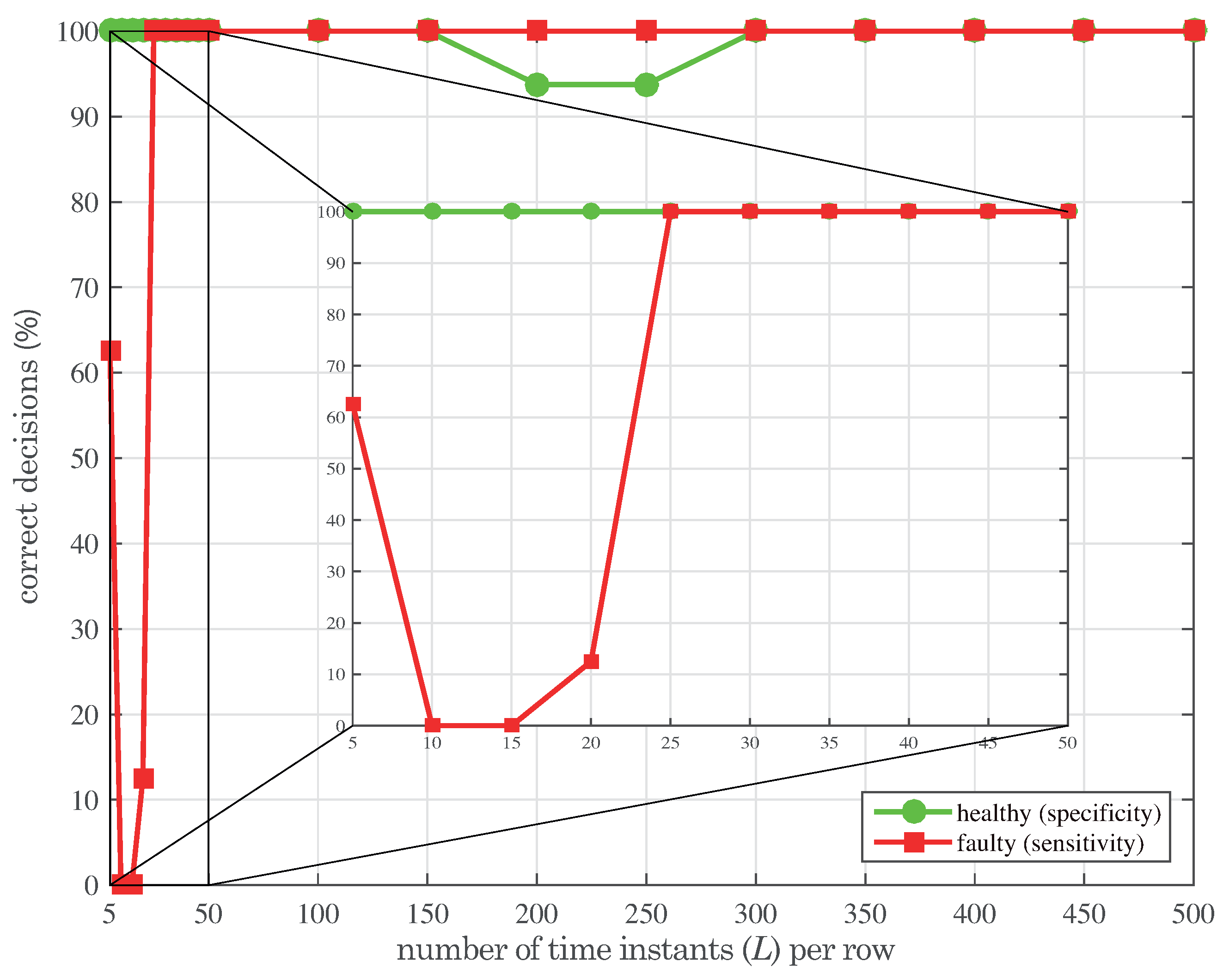
The sensitivity and specificity can also be used here as two statistical measures to analyze the performance of the test. On one hand, the sensitivity or power of the test is defined as the ratio of samples from the faulty wind turbine correctly classified. Therefore, if the false negative rate is defined as γ, the sensitivity is computed as $1-\gamma$. On the other hand, the specificity of the test can be defined as the percentage of samples from the healthy wind turbine correctly identified as such and is usually expressed as $1-\alpha$, where α is the false positive rate. These two measures are calculated—organized as detailed in

Table 7. Scheme for the presentation of the results in Table 8 (specificity and sensitivity).

	Healthy Sample (H0)	Faulty Sample (H1)
Fail to reject $H_0$	Specificity ($1-\alpha$)	False negative rate (γ)
Reject $H_0$	False positive rate (α)	Sensitivity ($1-\gamma$)

—in

Table 8. Sensitivity and specificity of the test for each of the four scores when the size of the samples to diagnose is $\nu =50$ and the sensors used are numbers $1,2,4,5,6$ and 7.

	Score 1		Score 2		Score 3		Score 4
	H0	H1	H0	H1	H0	H1	H0	H1
Fail to reject $H_0$	1.00	0.00	0.50	0.12	0.56	0.00	0.81	0.12
Reject $H_0$	0.00	1.00	0.50	0.88	0.44	1.00	0.19	0.88

with respect to the 24 samples and for the first four scores. The results in Table 8 show that the sensitivity $1-\gamma$ of the test is, on average, $94\%$, which is very close to $100\%$. Sensitivities of $100\%$ are achieved when scores 1 and 3 are considered. The mean value of the the specificity is $72\%$, which is very close to the expected value of $1-\alpha =64\%$, since the level of significance used in the test is $\alpha =36\%$. The specificity when only score 1 is considered is increased to $100\%$.

The reliability of the fault detection strategy can also be measured using the true rate of false negatives and the true rate of false positives. These two quantities are based on the Bayes theorem [20]. On one hand, the true rate of false positives is defined as the proportion of samples from the faulty wind turbine with respect to the samples that have been classified by the test as healthy, that is,

$$\begin{array}{c}\hfill P\left(H_1\right|\text{accept}{H}_0)\end{array}$$

On the other hand, the true rate of false negatives is defined as the proportion of samples from the healthy wind turbine with respect to those samples that have been classified by the test as faulty, that is,

$$\begin{array}{c}\hfill P\left(H_0\right|\text{accept}{H}_1)\end{array}$$

For the sensor configuration proposed in this section, the results—organized as described in

Table 9. Relationship between the proportion of false negatives and false positives and scheme for the presentation of the results in Table 10.

	Healthy Sample (H0)	Faulty Sample (H1)
Fail to reject $H_0$	P($H_0|\mathrm{accept}{H}_0$)	true rate of false negatives   $P\left(H_1\right|\mathrm{accept}{H}_0)$
Reject $H_0$	true rate of false positives   $P\left(H_0\right|\mathrm{accept}{H}_1)$	P($H_1|\mathrm{accept}{H}_1$)

—are summarized in

Table 10. True rate of false positives and false negatives for each of the four scores when the size of the samples to diagnose is $\nu =50$ and the sensors used are numbers $1,2,4,5,6$ and 7.

	Score 1		Score 2		Score 3		Score 4
	H0	H1	H0	H1	H0	H1	H0	H1
Fail to reject $H_0$	1.00	0.00	0.89	0.11	1.00	0.00	0.93	0.07
Reject $H_0$	0.00	1.00	0.53	0.47	0.47	0.53	0.36	0.64

.

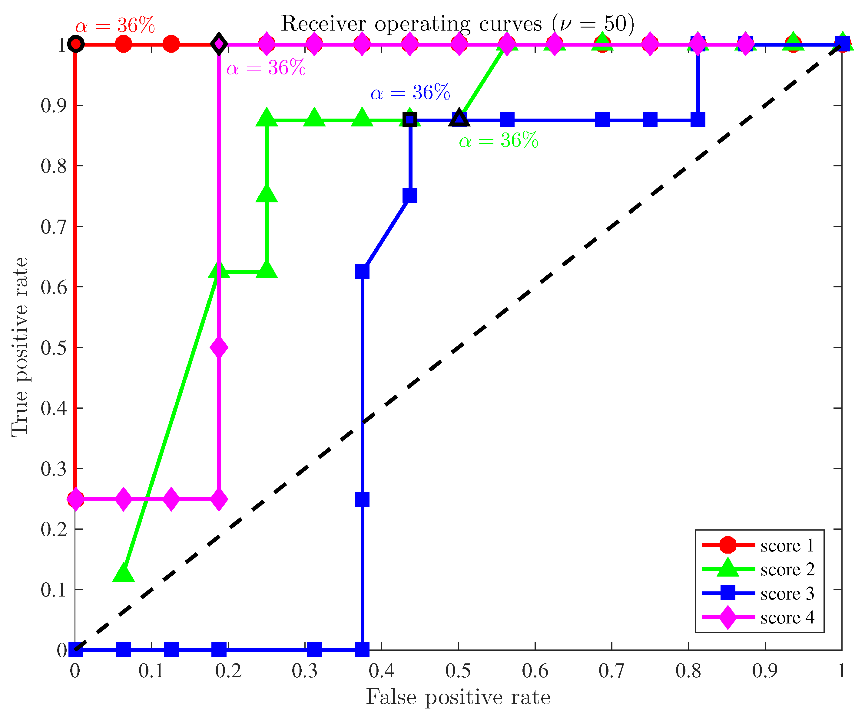
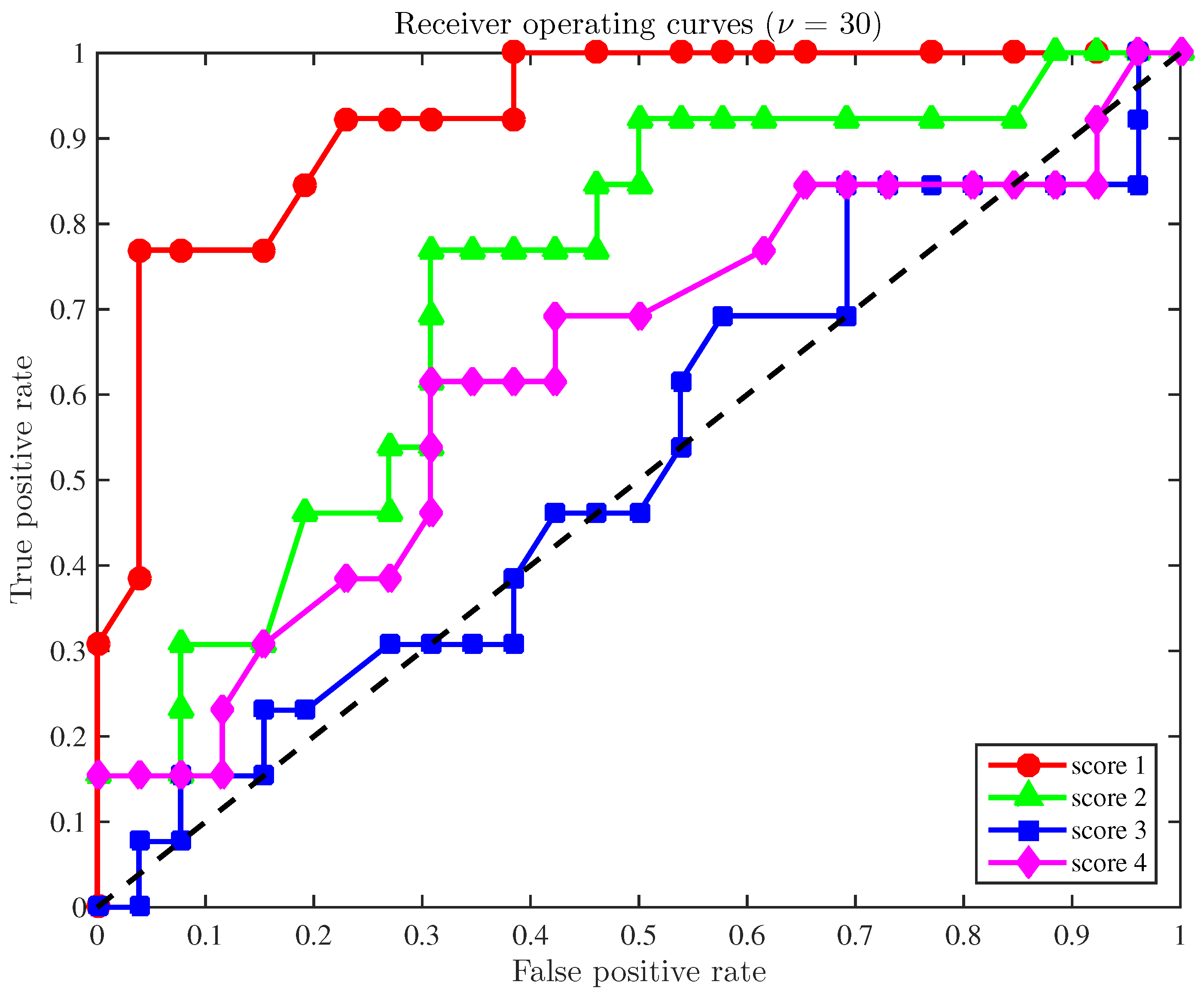
A final study is developed here based on the receiver operating curves (ROC) to demonstrate the overall accuracy of the fault detection strategy applied to a configuration with a reduced number of sensors. In general, these curves illustrate the compromise between the sensitivity and the false positive rate. More precisely, for a given level of significance and for each score, the pair of quantities

$$\begin{array}{c}\hfill (\text{false}\text{positive}\text{rate},\text{sensitivity})\in [0,1]\times [0,1]\subset {\mathbb{R}}^2\end{array}$$

is represented on a plane. As in [5], we have considered 49 levels of significance, ${\alpha }_1,\dots ,{\alpha }_{49}$, within the range $[0.02,0.98]$, where ${\alpha }_i=0.02\times i,i=1,\dots ,49$. The position of such points can be understood as follows. Since the ultimate goal is to reduce the quantity of false positives while the number of true positives is increased, these points must be ideally placed in the upper-left half plane. Therefore, a method is considered as satisfactory if those points lie within that upper-left half plane. 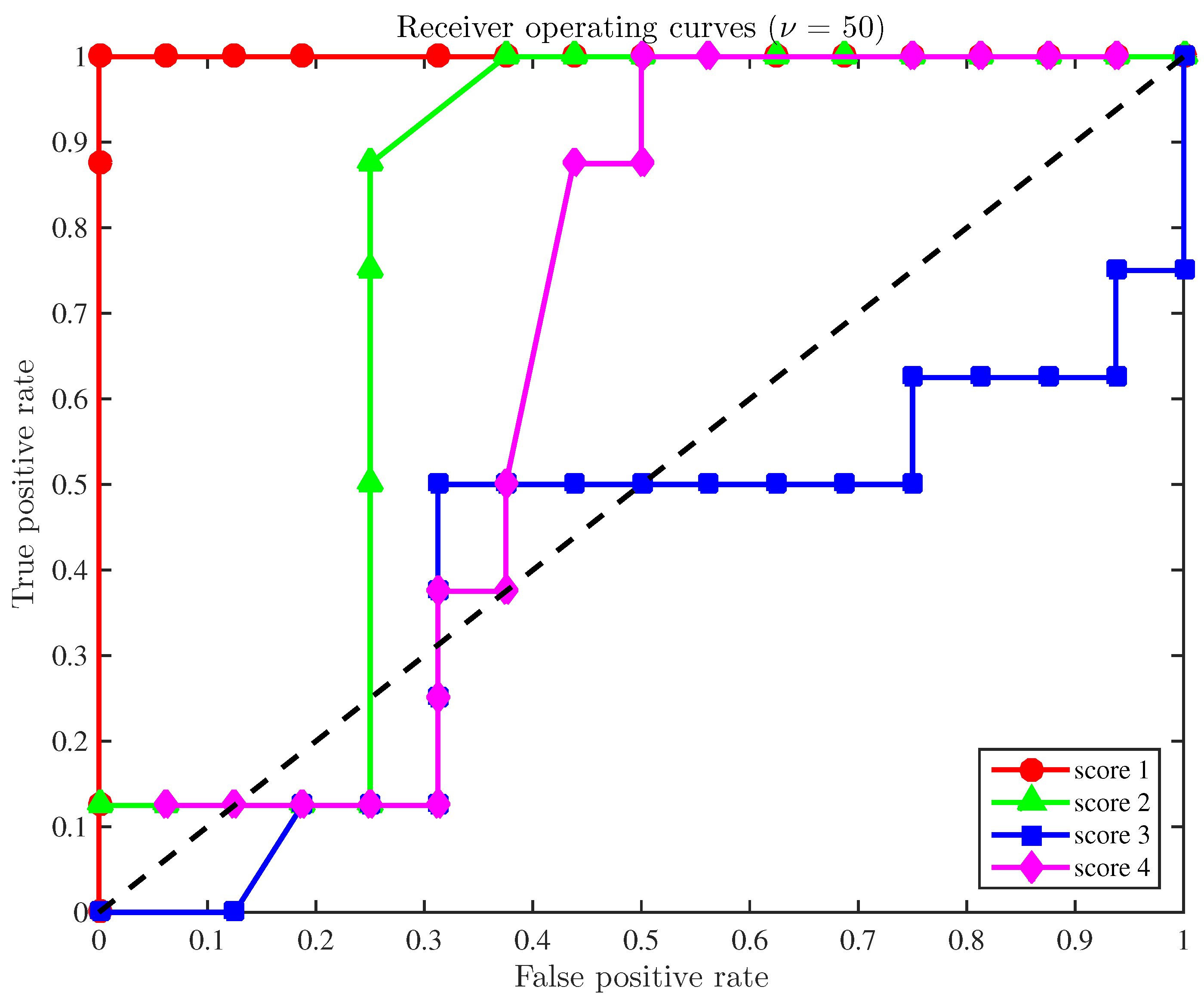In this sense, Figure 2 illustrates the receiver operating curves for the four scores when the size of the samples to diagnose is $\nu =50$ and the sensors used are numbers $1,2,4,5,6$ and 7. The ROCs for score 1 (in red, Figure 2) are particularly remarkable. The overall behavior of scores 2 and 4 are still acceptable, while the ROC for the third score must be considered as unsatisfactory.

The results of the fault detection strategy presented in this section, with respect to score 1 and using a reduced number of sensors (6 out of 13), when compared to the results in [5]—when the 13 sensors are used—do not present any performance degradation. That is, in both cases, we have a $100\%$ of accuracy in the detection of the 24 samples (healthy and faulty), but with about $54\%$ less sensors.

5. Detection Time Reduction Analysis

In the previous section, we have considered a strategy to reduce and select the number of sensors used in the fault detection strategy. It has been shown, for instance that, with $54\%$ less sensors, we are still able to accurately detect when the wind turbine is healthy or faulty. With the goal of the reduction of the detection time, in this section, we present an analysis of the effect of the structure of the matrix $\mathbf{Y}$ in Equation (8) with respect to number of rows (ν), number of columns (L), detection time (basically $(\nu \times L-1)\Delta$ seconds) and accuracy in the detection. The detection time is basically the time of collection since the computational time involved in the mathematical operations needed once the data is collected is comparatively quite small. Consequently, the detection time can be reduced if we reduce: (i) the number of rows (ν) of matrix $\mathbf{Y}$, that is, the size of the samples; (ii) the number of columns (L) of matrix $\mathbf{Y}$, that is, the number of time instants per row; or (iii) both ν and L. The effect of these reductions on the accuracy of the fault detection strategy will be analyzed in the following subsections, where all the available sensors are used.

5.1. On the Size of the Sample (ν)

The first way to study the detection time is the reduction of the size of the sample. The size of the sample has a physical meaning in our system: the information stored in the matrix is the data collected by the sensors, and therefore the smaller the size is, the lesser time the data must be acquired. The original Y matrix is formed by the data from all 13 sensors, and the information fulfills the matrix as detailed in Equation (8). This matrix is formed by submatrices of $\nu =50$ rows and $L=500$ columns, one for each sensor. Therefore, as said before, if there is a reduction on the size of the sample (ν), the total diagnosing time is reduced.

To analyze the effect on the overall performance of the fault detection strategy with a reduced number of rows, we will study a total of 10 different scenarios, corresponding to 10 different values for ν:

$$\begin{array}{c}\hfill {\nu }_1=5,{\nu }_2=10,\dots ,{\nu }_i=5i,\dots ,{\nu }_{10}=50\end{array}$$

For each scenario, we will study a different number of samples of $\nu ={\nu }_i,i=1,\dots ,10$ elements each, corresponding to the following distribution:

• $⌊\frac{48001}{{\nu }_i\times L}⌋$ samples of a faulty wind turbine with respect to each of the 8 particular fault scenarios defined in Table 3, resulting in a total of $8\times ⌊\frac{48001}{{\nu }_i\times L}⌋$ faulty samples, where $\lfloor ·\rfloor$ is the floor function and $L=500$, and
• $16\times ⌊\frac{48001}{{\nu }_i\times L}⌋$ samples of a healthy wind turbine,

which is also detailed in

Table 11. For each scenario, we will study a different number of faulty and healthy samples of $\nu ={\nu }_i,i=1,\dots ,10$ elements each.

	Faulty Samples	Healthy Samples
${\nu }_1=5$	$19\times 8=152$	304
${\nu }_2=10$	$9\times 8=72$	144
${\nu }_3=15$	$6\times 8=48$	96
${\nu }_4=20$	$4\times 8=32$	64
${\nu }_5=25$	$3\times 8=24$	48
${\nu }_6=30$	$3\times 8=24$	48
${\nu }_7=35$	$2\times 8=16$	32
${\nu }_8=40$	$2\times 8=16$	32
${\nu }_9=45$	$2\times 8=16$	32
${\nu }_{10}=50$	$1\times 8=8$	16

. The positive integer $⌊\frac{48001}{{\nu }_i\times L}⌋$ comes from the fact that we have simulated, for each fault scenario, the wind turbine during $(48001-1)\times \Delta =600$ seconds. This way, we can create $⌊\frac{48001}{{\nu }_i\times L}⌋$ samples of ${\nu }_i$ rows each.

In order to analyze the effect on the accuracy of the fault detection strategy, the sensitivity and specificity have been studied for the 10 different scenarios, corresponding to 10 different values for ν. As defined in Section 4.3, the specificity is the percentage of correct decisions when the sample studied is healthy (a healthy sample is set as healthy, hence failing to reject $H_0$), whereas the sensitivity is the percentage of faulty samples ($H_1$) rejected to be healthy.

As can be seen in Figure 3, the sensitivity and specificity change drastically when varying ν. Therefore, there is a direct connection between the correct decisions and the size of the sample. It can be seen that when the size (ν) decreases, the specificity (that is, out of the $8\times ⌊48001/({\nu }_i\times L)⌋$ healthy samples, how many of them are detected as healthy) decreases rapidly from its maximum (a $100\%$ effectivity at $\nu =50$) to values around $50\%$ when the size is half its initial value. Therefore, the results get worse as soon as the size of the sample decreases from 50. However, the sensitivity (how many of the $⌊48001/({\nu }_i\times L)⌋$ faults are detected correctly) maintains a pretty good effectivity from sizes between 25 and 50, but then decreases to approximately $75\%$ accuracy.

If we examine the ROC curves in Figure 4, Figure 5 and Figure 6 for three different values of ν ($\nu =50,\nu =30$ and $\nu =10$, respectively), we see that, when $\nu =50$, the first score has a perfect performance, as it is always detecting both faulty and healthy situations. However, as ν decreases, there is a degradation in all scores, and, therefore, the results obtained are not as good as desired.

As a conclusion to this study, it is suggested that the size of the sample, that is, the number of rows of matrix $\mathbf{Y}$ in Equation (8), cannot be reduced from 50. This quantity is the minimum value with the maximum accuracy, and the results get much worse as soon as it began being reduced. This result is consistent with the general theory of statistical hypothesis testing [19], where the power or sensitivity of a test and the sample size are shown to be related.

5.2. On the Time Instants per Row (L)

The second possibility to reduce the time of diagnosis is to decrease the number of columns in the original matrix $\mathbf{Y}$ in Equation (8). Each column represents a different time instant. Therefore, the bigger number of columns the matrix needs, the more time instants the sensor must collect as information before processing it. To analyze the effect on the accuracy of the fault detection strategy, the reduction in the number of columns is made keeping the number of rows as $\nu =50$.

To analyze the effect on the overall performance of the fault detection strategy with a reduced number of columns, we will study a total of 19 different scenarios, corresponding to 19 different values for L:

$$\begin{array}{c}\hfill L_1=5,L_2=10,L_3=15,\dots ,L_{10}=50\end{array}$$

$$\begin{array}{c}\hfill L_{11}=100,L_{12}=150,L_{13}=200,\dots ,L_{19}=500\end{array}$$

For each scenario, we will study a total of 24 samples of $\nu =50$ elements each, corresponding to the following distribution:

• 16 samples of a healthy wind turbine, and
• Eight samples of a faulty wind turbine with respect to each of the eight particular fault scenarios defined in Table 3.

The results of this analysis can be summarized as follows:

• There is no direct connection between the decrease of the number of time instants and the specificity and the sensitivity. Hence, the detection is maintained to values of $100\%$ of effectivity of detection in both healthy and faulty samples (Figure 7), except for $L=200$ and $L=250$, when there are $6.25\%$ of false alarms (which can be considered a quite good performance), and for values of L smaller than 25.
• It can also be observed from Figure 7 that the first principal component (score 1) has a perfect recognition of the faulty samples of the wind turbine, as its detection is always $100\%$ when L is greater or equal to 25.
• As it can be inferred from the ROC curves in Figure 8 and Figure 9, the first principal component keeps, in both cases, a very good overall performance.

As a conclusion to this study, we can infer that the number of columns (L, time instants) can be reduced up to 25 without a degradation in the overall performance. Therefore, the detection time can be reduced from $312.4875$ seconds to only $15.6125$ seconds, that is, a reduction of $95\%$ of the original detection time.

6. Fault Detection with a Reduced Number of Sensors and a Reduced Number of Time Instants (L)

In this section, we will present two examples considering a fault detection strategy with a reduced number of sensors, as stated in Section 4, and also a reduced number of time instants ($L_a=50$ and $L_b=25$), as considered in Section 5.2. The purpose of this example is to prove that both simplifications altogether follow the objective of fault detection, without missing faults nor false alarms, and with a clear reduction in detection time and computational effort.

To analyze the effect on the overall performance of the fault detection strategy with a reduced number of sensors and with $L_a=50$ and $L_b=25$ time instants per row, we will study a total of 24 samples of $\nu =50$ elements each, respectively, corresponding to the following distribution:

• 16 samples of a healthy wind turbine, and
• Eight samples of a faulty wind turbine with respect to each of the eight particular fault scenarios defined in Table 3.

In both cases, the following combination of $\sigma =6$ sensors is considered:

• sensors $1,2,4,5,6$ and 7, that is, we will measure and collect the information provided by the generated electrical power, rotor speed, generator torque and the first, second and third pitch angles.

For the first case, each sample of $\nu =50$ elements is formed by the measures gathered from the sensors during $(\nu \times L_a-1)\Delta =31.24875$ seconds, where $L_a=50$ and the sampling rate $1/\Delta =80$ Hz. For the second case, each sample of $\nu =50$ elements is formed by the measures gathered from the sensors during $(\nu \times L_b-1)\Delta =15.6125$ seconds, where $L_b=50$ and the same sampling rate as in the first case.

For the first case ($L_a=50$), the results of the fault detection strategy are summarized in

Table 12. Categorization of the samples with respect to the presence or absence of a fault and the result of the test for each of the four scores when the size of the samples to diagnose is $\nu =50$, $L_a=50$, and the sensors used are numbers $1,2,4,5,6$ and 7.

	Score 1		Score 2		Score 3		Score 4
	H0	H1	H0	H1	H0	H1	H0	H1
Fail to reject $H_0$	16	0	9	0	5	0	7	0
Reject $H_0$	0	8	7	8	11	8	9	8

and

Table 13. True rate of false positives and false negatives for each of the four scores when the size of the samples to diagnose is $\nu =50$ and the sensors used are numbers $1,2,4,5,6$ and 7.

	Score 1		Score 2		Score 3		Score 4
	H0	H1	H0	H1	H0	H1	H0	H1
Fail to reject $H_0$	1.00	0.00	0.56	0.00	0.31	0.00	0.44	0.00
Reject $H_0$	0.00	1.00	0.44	1.00	0.69	1.00	0.56	1.00

. These results clearly exposed that the first principal component is capable of detecting all the faulty samples, and, at the same time, it is capable to state that all 16 healthy samples come from a wind turbine working on their normal condition. Thus, there are neither missing faults, which is a major problem in wind turbines, nor false alarms.

For the second case ($L_b=25$), the results for the first score are summarized in

Table 14. Categorization of the samples with respect to the presence or absence of a fault and the result of the test for the first score when the size of the samples to diagnose is $\nu =50$, $L_b=25$, and the sensors used are numbers $1,2,4,5,6$ and 7.

	Score 1		Score 1
	H0	H1	H0	H1
Fail to reject $H_0$	16	0	1.00 (specificity)	0.00
Reject $H_0$	0	8	0.00	1.00 (sensitivity)

. Even for this case, when the fault detection scheme is based on the measured gathered from the sensors during less than 16 seconds, the strategy is able to correctly classify a 100% of the samples both coming from the healthy and faulty wind turbine. More precisely, with 54% less sensors and 95% less detection time—compared to [5]—the fault detection strategy is still able to accurately detect when the wind turbine is healthy or faulty.

7. Conclusions

The proposed strategy, using only six sensors when $\nu =50$ and $L=25$, detects all the studied faults with a detection time of $15.6125$ s and with no false positive detections nor missed detections.

On one hand, compared to the five solutions to the problem given in [15], our strategy reduces the detection time for all the pitch actuator faults (that is, faults 1, 2, and 3), and for the scaling pitch angle sensor fault (fault 7). In the case of faults 4, 5, 6 and 8, our detection time is not the best nor the worst (again, compared to the five solutions given in [15]). However, it is noteworthy that, for all the studied faults, our fault detection scheme is the only one that achieves, in all cases, sensitivity and specificity of 100%.

On the other hand, compared to [5], with 54% less sensors and 95% less detection time, the real-time application of the fault detection method is now possible while still being able to detect when the wind turbine is healthy or faulty with a sensitivity and specificity of 100%.

References

1. Association, E.W.E. Wind in Power: 2015 European Statistics; European Wind Energy Association: Brussels, Belgium, 2016. [Google Scholar]
2. Jensen, P.H.; Fugleberg, K. Wind Energy Research Strategy by Danish Research Consortium for Wind Energy; Technical Report; Danish Research Consortium for Wind Energy: Roskilde, Denmark, 2015. [Google Scholar]
3. Van Kuik, G.; Peinke, J.; Nijssen, R.; Lekou, D.; Mann, J.; Sørensen, J.N.; Ferreira, C.; van Wingerden, J.; Schlipf, D.; Gebraad, P.; et al. Long-term research challenges in wind energy—A research agenda by the European Academy of Wind Energy. Wind Energy Sci. 2016, 1, 1–39. [Google Scholar] [CrossRef] [Green Version]
4. Crabtree, C.J.; Zappalá, D.; Tavner, P.J. Survey of commercially available condition monitoring systems for wind turbines. Available online: http://dro.dur.ac.uk/12497/ (accessed on 1 July 2016).
5. Pozo, F.; Vidal, Y. Wind Turbine Fault Detection through Principal Component Analysis and Statistical Hypothesis Testing. Energies 2016, 9, 3. [Google Scholar] [CrossRef] [Green Version]
6. Chepuri, S.P.; Leus, G. Sensor selection for estimation, filtering, and detection. In Proceedings of the 2014 International Conference on Signal Processing and Communications (SPCOM), Bangalore, India, 22–25 July 2014; pp. 1–5.
7. Bai, C.Z.; Katewa, V.; Gupta, V.; Huang, Y.F. A stochastic sensor selection scheme for sequential hypothesis testing with multiple sensors. IEEE Trans. Signal Process. 2015, 63, 3687–3699. [Google Scholar] [CrossRef]
8. Miao, J.; Zhang, T.; Wang, Y.; Li, G. Optimal Sensor Selection for Classifying a Set of Ginsengs Using Metal-Oxide Sensors. Sensors 2015, 15, 16027–16039. [Google Scholar] [CrossRef] [PubMed]
9. Wang, Y.; Ma, X.; Malcolm, J. Optimal sensor selection for wind turbine condition monitoring using multivariate principal component analysis approach. In Proceedings of the 2012 18th International Conference on Automation and Computing (ICAC), Loughborough, UK, 7–8 September 2012; pp. 1–7.
10. Jolliffe, I.T. Discarding variables in a principal component analysis. I: Artificial data. J. R. Stat. Soc. Ser. C (Appl. Stat.) 1972, 21, 160–173. [Google Scholar] [CrossRef]
11. Jonkman, J. NWTC Computer-Aided Engineering Tools (FAST), version v7; National Wind Technology Center: Boulder, CO, USA, Last modified 28 October 2013.
12. Odgaard, P.; Johnson, K. Wind Turbine Fault Diagnosis and Fault Tolerant Control—An Enhanced Benchmark Challenge. In Proceedings of the 2013 American Control Conference–ACC, Washington, DC, USA, 17–19 June 2013; pp. 1–6.
13. Jonkman, J.M.; Butterfield, S.; Musial, W.; Scott, G. Definition of a 5-MW Reference Wind Turbine for Offshore System Development; Technical Report NREL/TP-500-38060; National Renewable Energy Laboratory: Golden, CO, USA, 2009.
14. Kelley, N.; Jonkman, B. NWTC Computer-Aided Engineering Tools (Turbsim), version 1.06.00; National Wind Technology Center: Boulder, CO, USA, Last modified 30 May 2013.
15. Odgaard, P.F.; Stoustrup, J.; Kinnaert, M. Fault-tolerant control of wind turbines: A benchmark model. IEEE Trans. Control Syst. Technol. 2013, 21, 1168–1182. [Google Scholar] [CrossRef]
16. Liniger, J.; Pedersen, H.C.; Soltani, M. Reliable Fluid Power Pitch Systems: A Review of State of the Art for Design and Reliability Evaluation of Fluid Power Systems. In Proceedings of the ASME/BATH 2015 Symposium on Fluid Power and Motion Control, Chicago, IL, USA, 12–14 October 2015; p. V001T01A026.
17. Chaaban, R.; Ginsberg, D.; Fritzen, C.P. Structural Load Analysis of Floating Wind Turbines Under Blade Pitch System Faults. In Wind Turbine Control and Monitoring; Luo, N., Vidal, Y., Acho, L., Eds.; Springer International Publishing: Cham, Switzerland, 2014; pp. 301–334. [Google Scholar]
18. Chen, L.; Shi, F.; Patton, R. Active FTC for hydraulic pitch system for an off-shore wind turbine. In Proceedings of the 2013 Conference on Control and Fault-Tolerant Systems (SysTol), Nice, France, 9–11 October 2013; pp. 510–515.
19. Ugarte, M.D.; Militino, A.F.; Arnholt, A. Probability and Statistics with R; Chemical Rubber Company (CRC) Press: Boca Raton, FL, USA, 2008. [Google Scholar]
20. DeGroot, M.H.; Schervish, M.J. Probability and Statistics; Pearson: Boston, MA, USA, 2012. [Google Scholar]
Figure 1. The fault detection strategy is based on testing for notable changes in the distributions of the sample coming from the healthy wind turbine and the sample coming from the current wind turbine to diagnose [5].
Energies 09 00520 g001
Figure 2. The receiver operating curves (ROCs) for the four scores when the size of the samples to diagnose is ν = 50 and the sensors used are numbers 1 , 2 , 4 , 5 , 6 and 7. The pair (false positive rate, sensitivity) R 2 is emphasized—with a black border—for the four scores when the level of significance is α = 36 % .
Energies 09 00520 g002
Figure 3. Specificity (green) and sensitivity (red) of the test as a function of the size of the sample (ν), that is, the number of rows of matrix Y in Equation (8), when the first score is used.
Energies 09 00520 g003
Figure 4. The ROCs for the four scores when the size of the samples to diagnose is ν = 50 and all the sensors are used.
Energies 09 00520 g004
Figure 5. The ROCs for the four scores when the size of the samples to diagnose is ν = 30 and all the sensors are used.
Energies 09 00520 g005
Figure 6. The ROCs for the four scores when the size of the samples to diagnose is ν = 10 and all the sensors are used.
Energies 09 00520 g006
Figure 7. Specificity (green) and sensitivity (red) of the test as a function of the number of time instants per row (L) when the first score is used.
Energies 09 00520 g007
Figure 8. The ROCs for the four scores when the number of time instants per row is L = 500 .
Energies 09 00520 g008
Figure 9. The ROCs for the four scores when the number of time instants per row is L = 100 .
Energies 09 00520 g009