Dynamic Prediction of Power Storage and Delivery by Data-Based Fractional Differential Models of a Lithium Iron Phosphate Battery

Abstract

A fractional derivative system identification approach for modeling battery dynamics is presented in this paper, where fractional derivatives are applied to approximate non-linear dynamic behavior of a battery system. The least squares-based state-variable filter (LSSVF) method commonly used in the identification of continuous-time models is extended to allow the estimation of fractional derivative coefficents and parameters of the battery models by monitoring a charge/discharge demand signal and a power storage/delivery signal. In particular, the model is combined by individual fractional differential models (FDMs), where the parameters can be estimated by a least-squares algorithm. Based on experimental data, it is illustrated how the fractional derivative model can be utilized to predict the dynamics of the energy storage and delivery of a lithium iron phosphate battery (LiFePO${}_4$) in real-time. The results indicate that a FDM can accurately capture the dynamics of the energy storage and delivery of the battery over a large operating range of the battery. It is also shown that the fractional derivative model exhibits improvements on prediction performance compared to standard integer derivative model, which in beneficial for a battery management system.

1. Introduction

Technological improvements in rechargeable solid-state batteries are recently being driven by an ever-increasing demand for electrical applications in automotive, power tools and communication systems. Among the various existing technologies, state-of-the-art lithium-ion (Li-ion) battery technologies are the default choice, providing one of the best energy-to-weight ratios, offering flexible and lightweight design, having low self-discharge when not in use and exhibiting little to no memory effect. All of these beneficial features, as well as decreasing costs, have made Li-ion batteries one of the primary candidates for the next generation of energy storage and delivery systems in portable electronics, electrified transportation, renewable energy integration, and smart grids [1,2,3,4,5,6,7].

Due to volatility, flammability and entropy changes, Li-ion batteries can cause irreversible, and under extreme conditions, catastrophic damages when overcharged or subjected to high discharge rates. Moreover, overcharging and overdischarging may reduce cell storage capacity and total cycle life of the battery due to irreversible chemical reactions [8,9,10]. Therefore, a battery management system (BMS) plays a vital role in improving battery performance and optimizing battery operation in a safe and reliable manner. A BMS is composed of hardware and software in order to protect the battery from operating outside its safe operating area, monitoring the state of the battery, and controlling its environment [11,12].

Some (Li-ion) battery model is required for designing and building BMS algorithms that uses this model to predict unmeasurable variables such as the state of charge (SOC) and state of health (SOH) of the battery. In addition, a BMS may be used to predict and compare measurable variables such as current, voltage, power and battery temperature [13,14,15,16,17] for battery fault and conditioning monitoring. An example of BMS usage can be seem in electric vehicle (EV) applications, shown in Figure 1. Indeed, among all the functions, one of the primary tasks of BMS is to track physical (un)measurable parameters and observe the states of the battery as the battery ages [18,19,20].

A BMS may use a physics-based battery model based on electrochemical principles [21] typically describing with a set of partial differential equations (PDE). A physics-based battery PDE model can account for the diffusion, intercalation, and electrical dynamics of a battery. A physics-based battery PDE model has the advantage of being able to describe detailed information in terms of integration of the various physical processes occurring in a battery and prediction capabilities, but may suffer from complexity and parameter uncertainty. Parameter estimation can be a solution to parameter uncertainty, but is limited by parameter identifiability conditions when only external voltage, current and temperature information is available.

With limited computing resources in a BMS for parameter estimation and model simulation, simplification of the electrochemical model can be done via the porous electrode model with a polynomial approximation model (PAM) and a single particle model (SPM) [23,24]. Although both PAM and SPM are computationally faster, they do not account for all physical processes. For example, the solution phase diffusion limitations are ignored, thus they have limitations in prediction of battery performance [25,26].

Another way for battery modeling is the simple equivalent circuit model (ECM), which is developed by using internal resistance, effective capacitance and equivalent potential to mimic the phenomenological behavior of batteries [27]. This model has a clear electrical interpretation. Unfortunately, the linearity and finite order of the ECM lacks the possibility to capture the possibly volatile and partial derivative nature of the electrochemical process over the full operating range of a Li-ion battery [28,29]. Although the accuracy of an ECM in predicting the input/output behavior of the battery can be improved by allowing the model parameters to vary with applied current, temperature and the SOC, the validity of the underlying ECM is still unreliable in high power and high energy applications. Especially for battery application in the automotive industry, where safety is critical for a high energy battery pack [30,31]

It is clear that alternative battery dynamic models with low computational requirements for the BMS are desired. A BMS may use a simplified dynamic model to capture battery dynamics formulated on the basis of observations from a power charge/discharge demand signal to the voltage and current signals [22]. Besides focusing on the dynamics of the electrochemical process of Li-ion battery, it is also very important to model the dynamics of battery energy storage capacity in terms of energy demand based on measurable input/output signals in real-time. From this point of view, a viable alternative method to model the battery system is to model the dynamic effects of power storage and delivery, as indicated in Figure 2. In this paper, such a dynamic model for power storage and delivery is based on fractional derivative model, used to capture the possible infinite dimensional behavior of battery power dynamics.

A recently published method for parameter estimation of a fractional differential model (FDM) for a battery system has shown the requirements of a large amount of convolution and integration calculations [32] that can be time consuming and sensitive to the noise on voltage and/or current measurements and the value of the fractional derivative.

The purpose of this paper is to show that: (a) the power storage/delivery dynamics of a Li-ion battery can be accurately modeled by a continuous-time FDM; and (b) optimization of parameters can be found via state variable filters (SVF) to generate smooth fractional derivatives of input/output signals that are less susceptible to noise. Based on filtered fractional derivative signals, the least squares-based state-variable filter (LSSVF) method [33] is utilized to identify the parameters of the FDM. The performance of the proposed method is evaluated on the FDM identification for energy storage and delivery of a lithium iron phosphate battery (LiFePO${}_4$).

As indicated in Figure 2, the proposed method to predict power delivery of a battery based FDM is done by modeling the individual dynamics from a power charge/discharge demand signal to the voltage and the current signals of a LiFePO${}_4$ battery, respectively. The models are combined to formulate a dynamic model of a battery as a power storage/delivery system to identify how fast a battery can store and deliver energy as a function of time.

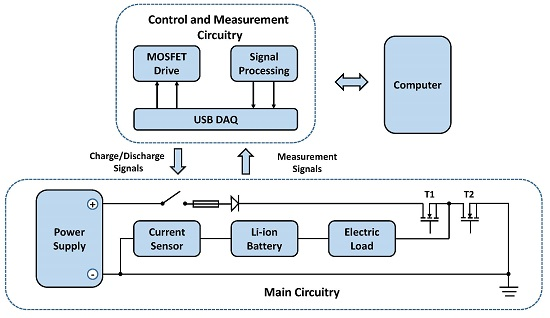
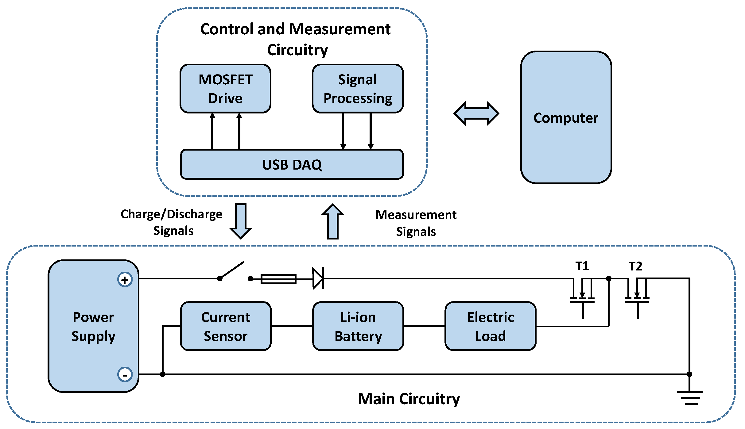
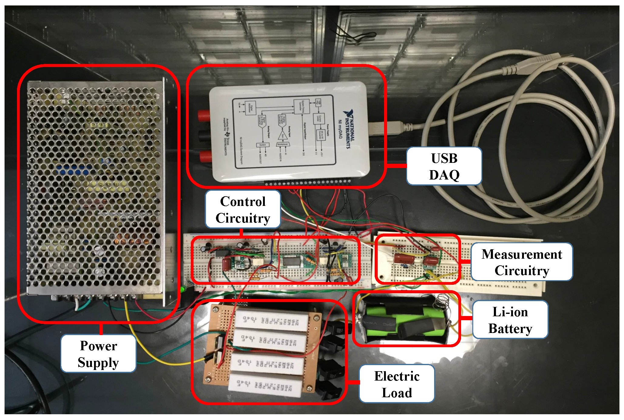
2. Experimental Setup

As shown in Figure 3, an experimental setup is built to test a battery as a power storage/delivery system. The charge/discharge demand signal can be applied as the input when measuring current and voltage signals of the batteries are recorded in real-time. There are three parts of the experimental setup: main circuitry, control and measurement circuitry, and computer.

In the main circuity, metal-oxide-semiconductor field-effect transistor (MOSFETs) T${}_1$ and T${}_2$ are used to allow the control of the power supply to Li-ion batteries. When T${}_1$ is on and T${}_2$ is off, the Li-ion battery is connected to the power supply. The power is transferred to charge the battery. When T${}_1$ is off and T${}_2$ is on, the battery is disconnected with the power supply. The power flow from the supply is switched off, thus the battery is connected to the ground and discharged. The main use of the pulse-width modulation (PWM) technique of T${}_1$ and T${}_2$ is to allow for modulating charge and discharge demand signals. The electric load is comprised of a parallel connection of load resistors. Such an electric load behaves to limit the current when the battery is charged, and performs as the load when the battery is discharged.

In the control and measurement circuitry, a National Instruments (NI, Austin, TX, USA) USB data acquisition (DAQ) device is used to delivery corresponding control signals to switch MOSFETs. The DAQ device is also applied to receive the measured signals and can communicate with the computer via a USB cable in real-time. A MOSFET drive is developed to boost the level of the digital output signal generated by the DAQ device. Low-order Butterworth low-pass filtering circuitry is used to reduce aliasing effects on the measured switching signals. a NI LabVIEW program was developed to automatically load cycle signals from existing files and can also save measured signals from the DAQ device. The experimental battery test can be repeated by applying the same sequence of charge/discharge demand signals.

A photograph of the experimental battery tester is shown in Figure 4. A 2.3 Ah-3.3 V LiFePO${}_4$ battery cell ANR26650 manufactured by A123 Systems (Waltham, MA, USA) is utilized in the experimental test. Pulse discharge at 10 s can reach 120 A and maximum continuous discharge is 70 A. Low drain-to-source on-resistance MOSFET IRLZ34 is applied to adapt in a high current flow. A bidirectional ± 20 A Hall effect sensor ACS714 is utilized to measure the current, and an analog-to-digital (A/D) conversion is used to measure the voltage over the battery.

3. Fractional Differential Systems

3.1. Fractional Differential System Equation

A fractional differential system is governed by a fractional differential equation

$$y\left(t\right)+a_1{D}^{{\mathsf{\alpha }}_1}y\left(t\right)+...+a_n{D}^{{\mathsf{\alpha }}_n}y\left(t\right)=b_0{D}^{{\mathsf{\beta }}_0}u\left(t\right)+b_1{D}^{{\mathsf{\beta }}_1}u\left(t\right)+...+b_m{D}^{{\mathsf{\beta }}_m}u\left(t\right)$$

(1)

where $(a_j,b_i)\in {\mathbb{R}}^2$, and the differentiation orders ${\mathsf{\alpha }}_1<{\mathsf{\alpha }}_2<...<{\mathsf{\alpha }}_n$, ${\mathsf{\beta }}_0<{\mathsf{\beta }}_1<...<{\mathsf{\beta }}_m$, and ${\mathsf{\alpha }}_i,{\mathsf{\beta }}_i\in {\mathbb{R}}^{+}$ are allowed to be non-integer positive real numbers. The concept of differentiation to an arbitrary non-integer order $\mathsf{\alpha }$ is defined as [34,35,36]

$$D^{\mathsf{\alpha }}={(\frac{\text{d}}{\text{d}t})}^{\mathsf{\alpha }},\forall \mathsf{\alpha }\in {\mathbb{R}}^{+}$$

The $\mathsf{\alpha }$-th order uninitialized fractional derivative of a function $f\left(t\right)$ is defined as an integer derivative of order $\lceil \mathsf{\alpha }\rceil$ of a non-integer integral of order $\mathsf{\alpha }-\lfloor \mathsf{\alpha }\rfloor$

$$D^{\mathsf{\alpha }}f\left(t\right)={(\frac{\text{d}}{\text{d}t})}^{\mathsf{\alpha }}\frac{1}{\mathsf{Г}(\lceil \mathsf{\alpha }\rceil -\mathsf{\alpha })}{\int }_0^t\frac{f\left(\mathsf{\tau }\right)}{{(t-\mathsf{\tau })}^{\mathsf{\alpha }-\lfloor \mathsf{\alpha }\rfloor }}\mathrm{d}\mathsf{\tau }$$

(2)

where $t>0,\forall \mathsf{\alpha }\in {\mathbb{R}}^{+}$, and Euler gamma function $\mathsf{Г}\left(\mathsf{\beta }\right)$ is defined for every $\mathsf{\beta }$ $\in {\mathbb{R}}^{+}$ by

$$\mathsf{Г}\left(\mathsf{\beta }\right)={\int }_0^{\infty }{z}^{\mathsf{\beta }-1}{\mathrm{e}}^{-z}\mathrm{d}z$$

(3)

In the above equations, $\lceil ·\rceil$ denotes the ceiling function that is defined as the smallest integer still greater than $\mathsf{\alpha }$, and $\lfloor ·\rfloor$ is the floor function that represents the largest integer still smaller than $\mathsf{\alpha }$. The Laplace transform

$$\mathcal{L}\left\{D^{\mathsf{\alpha }}f\left(t\right)\right\}=s^{\mathsf{\alpha }}F\left(s\right),\mathrm{if}f\left(t\right)=0\forall t\le 0$$

(4)

of $\mathsf{\alpha }$-th derivative ($\mathsf{\alpha }\in {\mathbb{R}}^{+}$) can also be used to describe a fractional systems [37,38]. With both the input signal $u\left(t\right)$ and the output signal $y\left(t\right)$ equal to 0 for all $t<0$, allows Equation (1) to be written in a transfer function form

$$G\left(s\right)=\frac{b_0{s}^{{\mathsf{\beta }}_0}+b_1{s}^{{\mathsf{\beta }}_1}+\cdots +b_m{s}^{{\mathsf{\beta }}_m}}{1+a_1{s}^{{\mathsf{\alpha }}_1}+\cdots +a_n{s}^{{\mathsf{\alpha }}_n}}$$

(5)

which represents the fractional order continuous-time transfer function $G\left(s\right)$ of the FDM throughout the paper.

3.2. Direct Least Squares Method

To consider estimation of the parameters in the FDM in Equation (1) or $G\left(s\right)$ in Equation (5), measurable output signals $y\left(t\right)$ are considered to be corrupted by an additive noise $e\left(t\right)$ given by

$$y\left(t\right)=y_0\left(t\right)+e\left(t\right)$$

(6)

where $y_0\left(t\right)$ is hypothetical noise-free deterministic system output. The input $u\left(t\right)$ and the output $y\left(t\right)$ signals are supposed to be related by Equation (1) and the equation error can be described as [39]

$$\mathsf{\epsilon }\left(t\right)=y\left(t\right)-\mathsf{\phi }{\left(t\right)}^T\mathsf{\theta }$$

(7)

where the regressor is given by

$$\mathsf{\phi }{\left(t\right)}^T=\left[D^{{\mathsf{\beta }}_0}u\left(t\right)D^{{\mathsf{\beta }}_1}u\left(t\right)...D^{{\mathsf{\beta }}_m}u\left(t\right)-D^{{\mathsf{\alpha }}_1}y\left(t\right)-D^{{\mathsf{\alpha }}_2}y\left(t\right)...-D^{{\mathsf{\alpha }}_n}y\left(t\right)\right]$$

(8)

and the parameter is denoted by the vector

$${\mathsf{\theta }}^T=[b_0{b}_1...b_m{a}_1{a}_2...a_n]$$

(9)

Minimizing the $L_2$ norm of $\mathsf{\epsilon }\left(t\right)$

$$J={\int }_0^T{\left(\mathsf{\epsilon }\left(t\right)\right)}^2\mathrm{d}t$$

(10)

with respect to $\mathsf{\theta }$, would lead to the following least squares (LS) estimate

$${\widehat{\mathsf{\theta }}}_{\text{LS}}={\left[\begin{array}{c}{\int }_0^T\mathsf{\phi }{\left(t\right)}^T\mathsf{\phi }\left(t\right)\mathrm{d}t\end{array}\right]}^{-1}{\int }_0^T\mathsf{\phi }{\left(t\right)}^{T}y\left(t\right)\mathrm{d}t$$

(11)

Clearly, a numerical discretization of the fractional derivatives of the input/ouput signals must be employed for the numerical computation of the estimate in Equation (11). With a time digitized regression vector $\mathsf{\phi }\left(k{T}_s\right),k=1,2,\dots ,N$ over N data points, we can formulate the regressor matrix

$$\mathsf{Ф}={\left[\mathsf{\phi }\left(T_s\right)\mathsf{\phi }\left(2T_s\right)\dots \mathsf{\phi }\left(N{T}_s\right)\right]}^T$$

(12)

Similarly, an output matrix $\mathbf{Y}$ can be defined as a column vector of the digitized system output $y\left(k{T}_s\right),k=1,2,\dots ,N$ over N data points to allow the LS estimation to be computed via

$${\widehat{\mathsf{\theta }}}_{\text{LS}}={\left({\mathsf{Ф}}^T\mathsf{Ф}\right)}^{-1}{\mathsf{Ф}}^T\mathbf{Y}$$

(13)

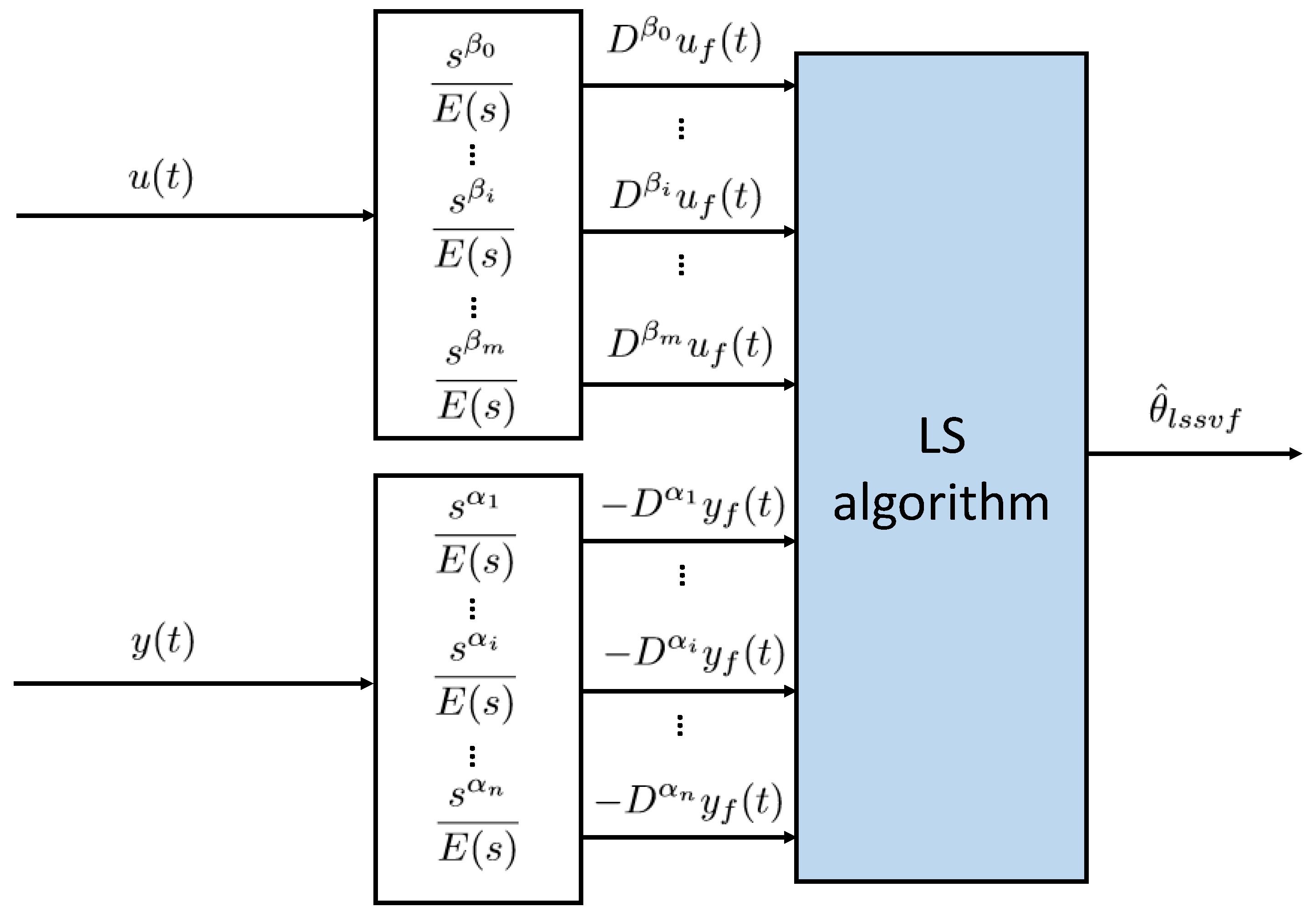
3.3. Least Squares-Based State-Variable Filter Method

Perturbations on either the initial conditions or the coefficients of a differential equation will typically lead to perturbations in the solution [35]. Special care needs to be given to the estimation of the coefficients of the FDM to reduce the effect of perturbations and/or noise on the input and output data. An effective way to estimate the coefficients of a continuous-time (fractional order) model is through a SVF [40,41,42]. From a signal analysis point of view, the SVF consists of multiple band-pass filters used to obtain the behavior of differentiation at low frequencies, while reducing the effect of noise at high frequencies. The SVF uses a common operator model [33,40]

$$L\left(s\right)=\frac{1}{E\left(s\right)}=\frac{1}{{(s+\lambda )}^n}$$

(14)

which is applied to pre-process the input and output signals

$$u_f\left(t\right)=L\left(s\right)u\left(t\right),y_f\left(t\right)=L\left(s\right)y\left(t\right)$$

(15)

where $u_f$ and $y_f$ are filtered input and output signals, respectively. The notion of an SVF can be extended to the (fractional) derivatives in Equation (1) to formulate a least squares-based SVF (LSSVF) method based on the filtered signals in

$$y_f\left(t\right)+a_1{D}^{{\mathsf{\alpha }}_1}{y}_f\left(t\right)+...+a_n{D}^{{\mathsf{\alpha }}_n}{y}_f\left(t\right)=b_0{D}^{{\mathsf{\beta }}_0}{u}_f\left(t\right)+b_1{D}^{{\mathsf{\beta }}_1}{u}_f\left(t\right)+...+b_m{D}^{{\mathsf{\beta }}_m}{u}_f\left(t\right)$$

(16)

Based on a filtered signal in Equation (16), the $L_2$ norm of ${\mathsf{\epsilon }}_f\left(t\right)$ now to be minimized is given by

$${\mathsf{\epsilon }}_f\left(t\right)=y_f\left(t\right)-{\mathsf{\phi }}_f{\left(t\right)}^T\mathsf{\theta }$$

(17)

where the regressor is given by the filtered input/output signals

$${\mathsf{\phi }}_f{\left(t\right)}^T=\left[D^{{\mathsf{\beta }}_0}{u}_f\left(t\right)D^{{\mathsf{\beta }}_1}{u}_f\left(t\right)\dots D^{{\mathsf{\beta }}_m}{u}_f\left(t\right)-D^{{\mathsf{\alpha }}_1}{y}_f\left(t\right)-D^{{\mathsf{\alpha }}_2}{y}_f\left(t\right)\dots -D^{{\mathsf{\alpha }}_n}{y}_f\left(t\right)\right]$$

(18)

Again, a numerical discretization of the (fractional) derivatives of the input/ouput signals must be employed for the numerical computation of a parameter estimate. More details on the computation of the digitized fractional derivatives follows in the next section. With a time digitized filtered regression vector ${\mathsf{\phi }}_f\left(k{T}_s\right),k=1,2,\dots ,N$ over N data points, we can formulate the LSSVF estimate as

$${\widehat{\mathsf{\theta }}}_{\text{LSSVF}}={\left({\mathsf{Ф}}_f^T{\mathsf{Ф}}_f\right)}^{-1}{\mathsf{Ф}}_f^T{\mathbf{Y}}_f$$

(19)

where

$${\mathsf{Ф}}_f={[{\mathsf{\phi }}_f\left(T_s\right){\mathsf{\phi }}_f\left(2T_s\right)...{\mathsf{\phi }}_f\left(N{T}_s\right)]}^T$$

(20)

and ${\mathbf{Y}}_f$ is a column vector of the filtered system output $y_f\left(k{T}_s\right),k=1,2,\dots ,N$ over N data points. The overall filtering and LS estimation in the LSSVF algorithm are summarized in Figure 5.

3.4. Computation of Digitized Fractional Derivatives

Time-analysis of a fractional derivative model, i.e., simulation of the system response to an arbitrary input signal, is carried out using a revised Grünwald-Letnikov definition. The revised Grünwald-Letnikov definition is given by

$$D^{\mathsf{\alpha }}f\left(t\right)=\underset{h\to 0}{lim}\frac{1}{h^{\mathsf{\alpha }}}\sum _{j=0}^{\left[\frac{t-a}{h}\right]}{(-1)}^j\left(\begin{array}{c}\mathsf{\alpha }\\ j\end{array}\right)f(t-jh)$$

(21)

where [·] donates the integer part. Usign the revised Grünwald-Letnikov definition, the closed-form numerical solution to the fractional-order differential Equation (1) is obtained in [43] by the recursive formulation

$$y_t=\frac{1}{{\sum }_{i=0}^n}\left(\begin{array}{c}{u}_t-\sum _{i=0}^n\frac{a_i}{h^{{\mathsf{\alpha }}_i}}\sum _{j=1}^{\left[\frac{t-a}{h}\right]}{w}_j^{\left({\mathsf{\alpha }}_j\right)}{y}_{t-jh}\end{array}\right)$$

(22)

where h is the step-size in computation, The function $w_j\left(\mathsf{\alpha }\right)$ in the recursive formulation of Equation (22) can be computed recursively from

$$w_0^{\mathsf{\alpha }}=1,w_j^{\mathsf{\alpha }}=(1-\frac{\mathsf{\alpha }+1}{j})w_{j-1}^{\mathsf{\alpha }},j=1,2,...$$

(23)

Using the above recursive formulations, the fractional derivatives of both the input and output signals can be calculated with Equation (22) and substituting ${(-1)}^{\mathsf{\alpha }}$ $\left(\begin{array}{c}\mathsf{\alpha }\\ j\end{array}\right)$ = $w_j^{\mathsf{\alpha }},$. Due to the fixed-step computation, the accuracy of the simulation may depend on the chosen step-size h, thus validating the results by gradually decreasing step-size h until there is no variation in the simulation results is desirable.

4. Power-Based Modeling

In order to establish a dynamic model of a Li-ion battery as a power storage/delivery system, the power charge/discharge demand signal $r\left(t\right)$ is considered as an input signal. The voltage signal $v\left(t\right)$ and current signal $i\left(t\right)$ of the battery are considered as observable output signals. As shown in Figure 2, the multiplication of voltage signal $v\left(t\right)$ and current signal $i\left(t\right)$ is equal to the power storage/delivery signal $p\left(t\right)$. The experimental results included below illustate that the parameters of the two separate FDMs between $r\left(t\right)$ as input signals and $v\left(t\right)$ and $i\left(t\right)$ as output signals can be estimated very well with the LSSVF method.

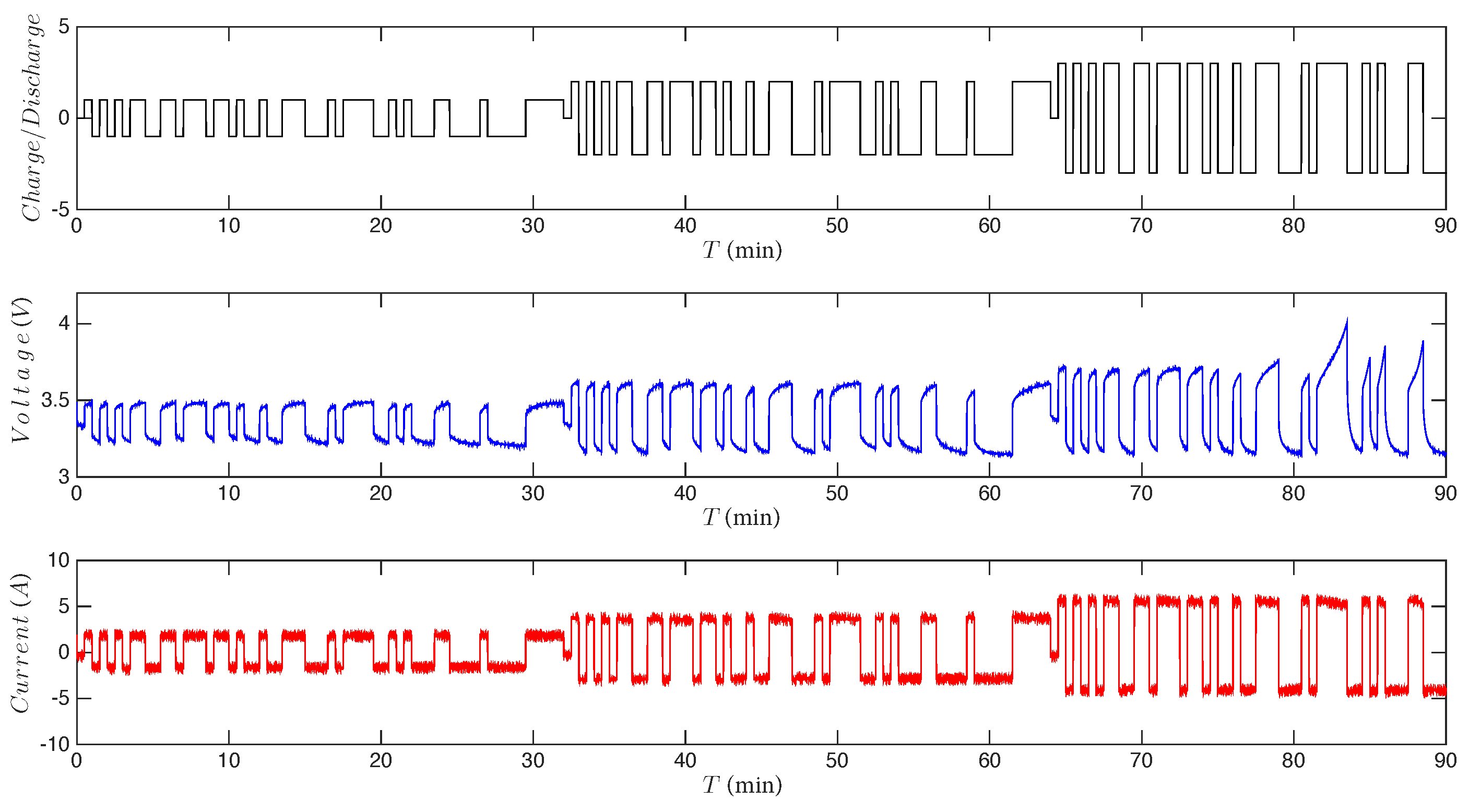
4.1. Experimental Results

For experimental verification of the parameter estimation of the battery FDM, the battery is charged and discharged by a sequence of charge/discharge demand signal composed of 6th order pseudo random binary sequence (PRBS) [22]. Specifically, each PRBS is the 6th order with different scaling factors of 1, 2, and 3, respectively. As a result, different C-rates are implemented in the experiment. Each PRBS is connected with a period of zero-state, which indicated the idle status of the charge/discharge system, as shown in Figure 6. The measured signals of voltage and current are also shown in Figure 6. The experimental time is T = 90 min, and the sample rate is 10 Hz, which contains 54,000 samples.

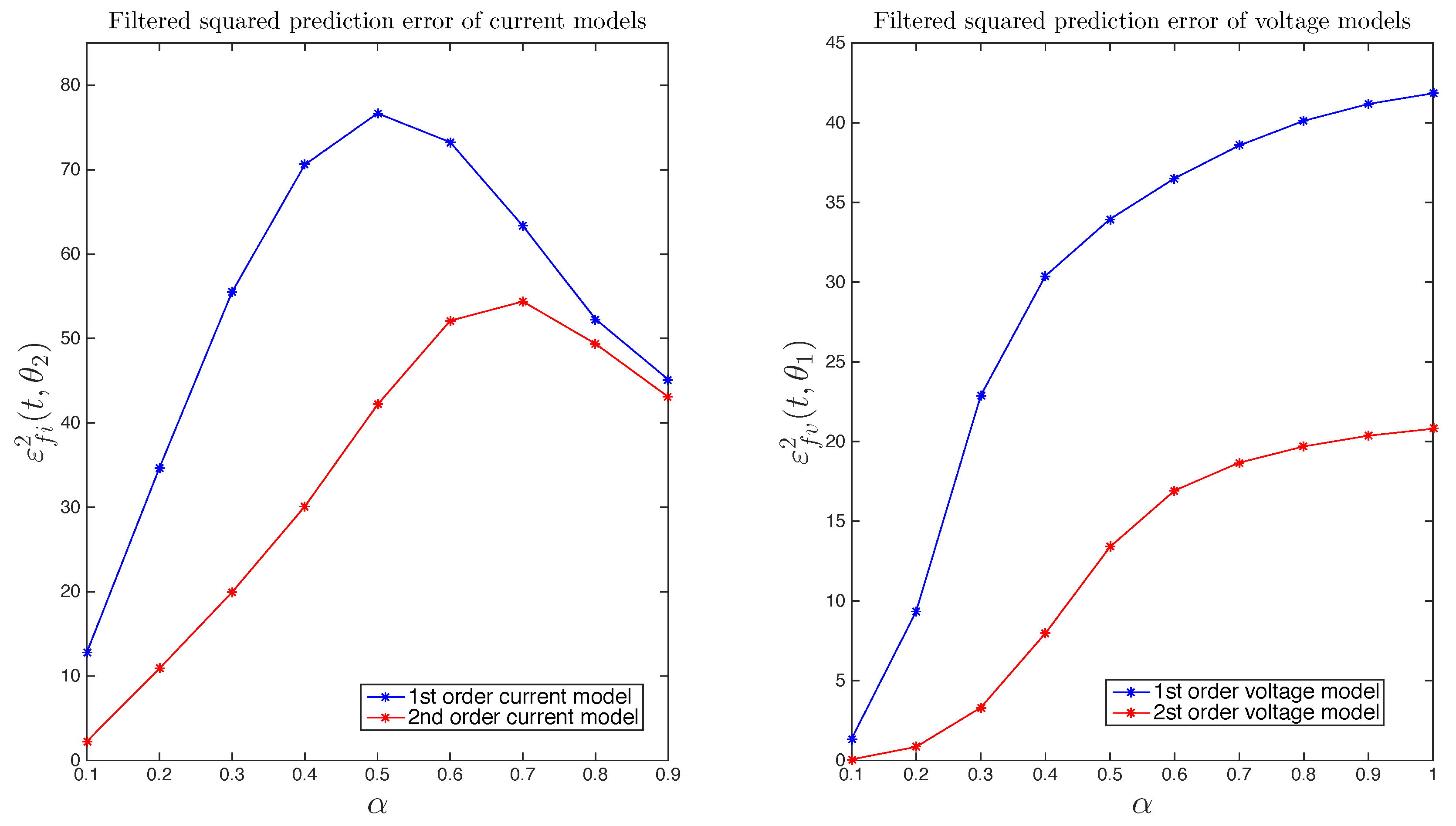
4.2. Voltage Model

A second-order voltage FDM, with input $r\left(t\right)$ and output $v\left(t\right)$, has much better prediction performance as shown in Figure 7,and the simplest form to capture the voltage dynamics is estimated by the LSSVF method in the form

$$v\left(t\right)=v_n\left(t\right)+v_0=\frac{b_2{s}^{2\mathsf{\alpha }}+b_1{s}^{\mathsf{\alpha }}+b_0}{a_2{s}^{2\mathsf{\alpha }}+a_1{s}^{\mathsf{\alpha }}+1}r\left(t\right)+v_0$$

(24)

where $v_0$ and $v_n\left(t\right)$ are offset voltage and new output voltage signals, separately. First order SVF $L\left(s\right)=\frac{1}{s+\mathsf{\lambda }}$ is then applied to get the filtered charge/discharge demand signal $r_f\left(t\right)$ and the filtered new output voltage signal $v_{nf}\left(t\right)$. In order to estimate the parameters, the filtered prediction error of voltage model can be defined as

$${\mathsf{\epsilon }}_{fv}(t,{\mathsf{\theta }}_1)=v_{nf}\left(t\right)-{\mathsf{\phi }}_{1f}^{*}{\left(t\right)}^T{\mathsf{\theta }}_1$$

(25)

where the regression vector is given by

$${\mathsf{\phi }}_{1f}^{*}{\left(t\right)}^T=[s^{2\mathsf{\alpha }}{r}_f\left(t\right)s^{\mathsf{\alpha }}{r}_f\left(t\right)r_f\left(t\right)-s^{2\mathsf{\alpha }}{v}_{nf}\left(t\right)-s^{\mathsf{\alpha }}{v}_{nf}\left(t\right)]$$

(26)

and the parameter vector

$${\mathsf{\theta }}_1^T=\left[b_2{b}_1{b}_0{a}_2{a}_1\right]$$

(27)

combines the unknown parameters.

subsequently, the predicted voltage

$$\widehat{v}(t,{\mathsf{\theta }}_1)={\widehat{v}}_n(t,{\mathsf{\theta }}_1)+v_0={\mathsf{\phi }}_{1f}^{*}{\left(t\right)}^T{\mathsf{\theta }}_1+v_0$$

(28)

is applied to estimate the performance of the model, where ${\widehat{v}}_n(t,{\mathsf{\theta }}_1)$ is the predicted new voltage. The filtered squared prediction error of voltage model given by

$${\mathsf{\epsilon }}_{fv}^2(t,{\mathsf{\theta }}_1)=\left|\right|v_{nf}\left(t\right)-{\widehat{v}}_n(t,{\mathsf{\theta }}_1){\left|\right|}_2^2$$

(29)

is utilized to validate the accuracy of the estimation.

4.3. Current Model

Following the same procedure, a first-order current FDM with the input $r\left(t\right)$ and the output $i\left(t\right)$, can be estimated by the LSSVF method to capture the current dynamics of battery. The first-order current FDM is of the from

$$i\left(t\right)=\frac{d_1{s}^{\mathsf{\alpha }}+d_0}{c_1{s}^{\mathsf{\alpha }}+1}r\left(t\right)$$

(30)

and still excellent prediction performance as shown in Figure 7.

After applying the same filter $L\left(s\right)$, the filtered current signal $i_f\left(t\right)$ and filtered charge/discharge demand signal $r_f\left(t\right)$ are used to minimize the $L_2$ norm of ${\mathsf{\epsilon }}_{fi}(t,{\mathsf{\theta }}_2)$

$${\mathsf{\epsilon }}_{fi}(t,{\mathsf{\theta }}_2)=i_f\left(t\right)-{\mathsf{\phi }}_{2f}^{*}{\left(t\right)}^T{\mathsf{\theta }}_2$$

(31)

where the regression vector is given by

$${\mathsf{\phi }}_{2f}^{*}{\left(t\right)}^T=[s^{\mathsf{\alpha }}{r}_f\left(t\right)r_f\left(t\right)-s^{\mathsf{\alpha }}{i}_f\left(t\right)]$$

(32)

and the parameter vector

$${\mathsf{\theta }}_2^T=\left[d_1{d}_0{c}_1\right]$$

(33)

combines the unknown coefficients in the first order current FDM. As in the voltage model, the filtered squared prediction error of current model is now built as

$${\mathsf{\epsilon }}_{fi}^2(t,{\mathsf{\theta }}_2)=\left|\right|i_f\left(t\right)-\widehat{i}(t,{\mathsf{\theta }}_2){\left|\right|}_2^2$$

(34)

to verify the accuracy of the model, where $\widehat{i}(t,{\mathsf{\theta }}_2)$ as the predicted current output.

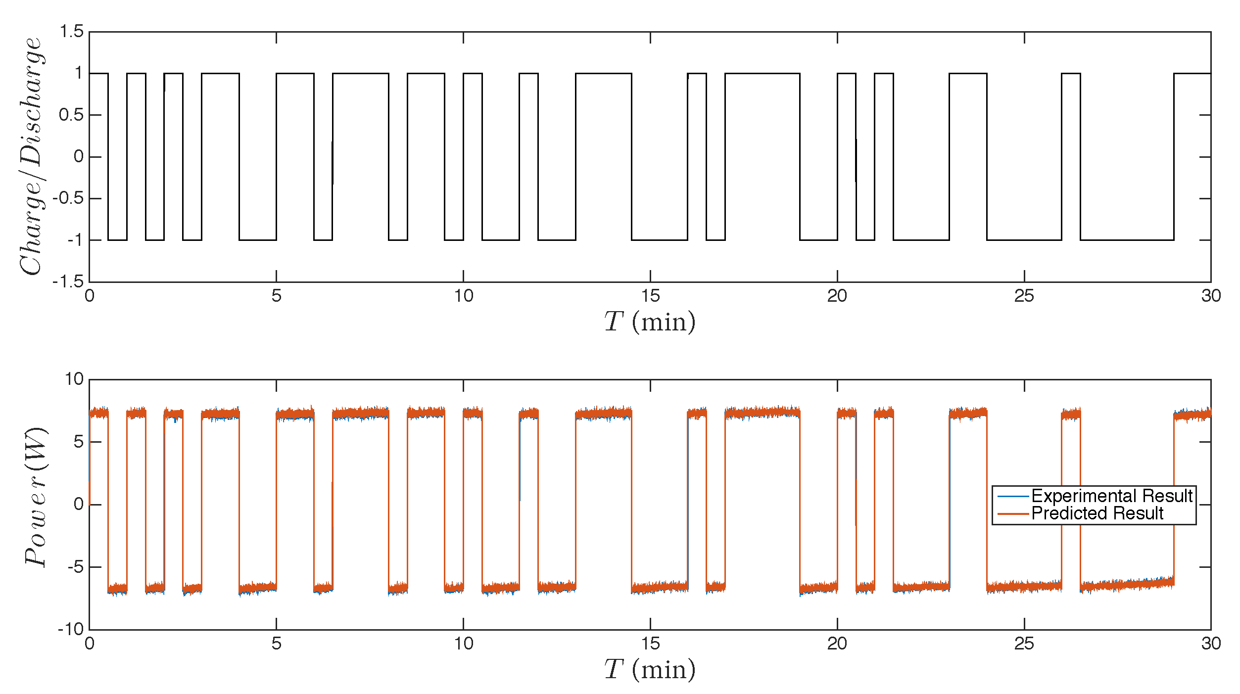
4.4. Experimental Data-Based Modeling

For identification and model validation purposes, the first 30 min of measured data and 5 Hz cut-off frequency SVF are applied to estimate the parameters and validate the models. The filtered squared prediction error of the first order and the second order voltage model ${\mathsf{\epsilon }}_{fv}^2$, and the current model ${\mathsf{\epsilon }}_{fi}^2$ as a function of fractional differential order $\mathsf{\alpha }$ are shown in Figure 7. The dependency on the fractional differential order $\mathsf{\alpha }$ is used to charactrize the accuracy of the models for different values of $\mathsf{\alpha }$, where a lower value along the y-axis indicates a more accurate estimation.

As can be seen in Figure 7, the results show that the filtered squared prediction error of a second-order voltage FDM is significantly smaller than a first-order model. This explains that the selected second-order model indeed has much better prediction performance, while still preserving the requirement of a model of the smallest complexity to capture the voltage dynamic. For the current FDM it is observed that a first order FDM suffices. Although the second-order current FDM has a slightly smaller prediction error, the first-order current FDM shows similar performance with the advantage of only having to need a first order model.

When the fractional differential order $\mathsf{\alpha }$ is chosen as $\mathsf{\alpha }=0.1$ both ${\mathsf{\epsilon }}_{fv}^2$ and ${\mathsf{\epsilon }}_{fi}^2$ have the smallest value, which leads to the most accurate estimation. Therefore, the fractional differential order $\mathsf{\alpha }$ = 0.1 is chosen in the system identification via the LSSVS method for both the voltage and current FDM in Equations (24) and (30). Fixing the fractional differential order, the batch-wise estimation leads to the following voltage model and the current model, respectively given by

• Voltage Model

  $$v\left(t\right)=\frac{0.2420s^{0.2}-0.3766s^{0.1}+0.1105}{1.7607s^{0.2}-2.9055s^{0.1}+1}r\left(t\right)+3.2141$$

  (35)
• Current Model

  $$i\left(t\right)=\frac{-1.7381s^{0.1}+2.1883}{-0.7840s^{0.1}+1}r\left(t\right)$$

  (36)

The estimated voltage FDM in Equation (35) and the current FDM in Equation (36) are used to predict the voltage, current outputs and power output on the basis of measurements of the charge/discharge demand signal $r\left(t\right)$ that acts as an input to these models. Prediction of the voltage and current signals is done with the parameters of the voltage and current FDMs in Equations (35) and (36) that have been optimized for 1-step-ahead prediction. The resulting 1-step-ahead predictions are given by

$$\widehat{v}\left(t\right|t-1)={\mathsf{\phi }}_1^{*}{\left(t\right)}^T{\mathsf{\theta }}_1+v_0$$

(37)

and

$$\widehat{i}\left(t\right|t-1)={\mathsf{\phi }}_2^{*}{\left(t\right)}^T{\mathsf{\theta }}_2$$

(38)

using the regessor vectors

$${\mathsf{\phi }}_1^{*}{\left(t\right)}^T=[s^{0.2}r\left(t\right)s^{0.1}r\left(t\right)r\left(t\right)-s^{0.2}{v}_n\left(t\right)-s^{0.1}{v}_n\left(t\right)]$$

(39)

and

$${\mathsf{\phi }}_2^{*}{\left(t\right)}^T=[s^{0.1}r\left(t\right)r\left(t\right)-s^{0.1}i\left(t\right)]$$

(40)

creating the 1-step-ahead power predictor by

$$\widehat{p}\left(t\right|t-1)=\widehat{v}\left(t\right|t-1)·\widehat{i}\left(t\right|t-1)$$

(41)

as a multiplication of the 1-step-ahead prediction of voltage and current.

It should be noted that the models given in Equations (35) and (36) may not be suitable for simulation, as parameters are optimized for prediction. Instead, the predictors in Equations (37) and (38) should be used for 1-step-ahead power delivery/storage prediction of the battery. As shown in Figure 8, the comparison of the predicted and measured results indicates that the estimated voltage and curent FDMs obtained via the LSSVF method can both capture the dynamics of the voltage and current signals of the battery system. Furthermore, the proposed method is evaluated to estimate the performance of FDM identification for power storage/delivery model, which is achieved by multiplying the outputs of the individual FDMs. As shown in Figure 9, the estimation results indicate that the power storage/delivery modelsis able to capture the dynamics of the battery as the power storage/delivery systems.

It should be noted that the one-step-ahead predictors using FDMs yield better prediction than using the same order integer models. The voltage and current prediction errors comparison between the optimized fractional models ($\mathsf{\alpha }=0.1$) given in Equations (35) and (36) and the integer models ($\mathsf{\alpha }=1$) given in Equations (24) and (30) are shown in Figure 10. The comparison result obtained indicates that very low relative voltage prediction errors and slight low current prediction errors of fractional models offer substantially better accuracy of prediction ability than integer models.

As a final comparision of the FDM quaility, a model fit ratio

$${\mathsf{\gamma }}_{x,x\in \{v,i,p\}}=(1-\frac{\parallel \widehat{x}\left(t\right|t-1)-x\parallel }{\parallel x-\overline{x}\parallel })$$

(42)

is introduced to validate the accuracy of the model, where x, $\overline{x}$ and $\widehat{x}\left(t\right|t-1)$ are output, mean value of output and one-step-ahead output predictor, respectively. Also shown in

Table 1. Model fit ratios comparison between fractional models ($\mathsf{\alpha }$ = 0.1) and integer models.

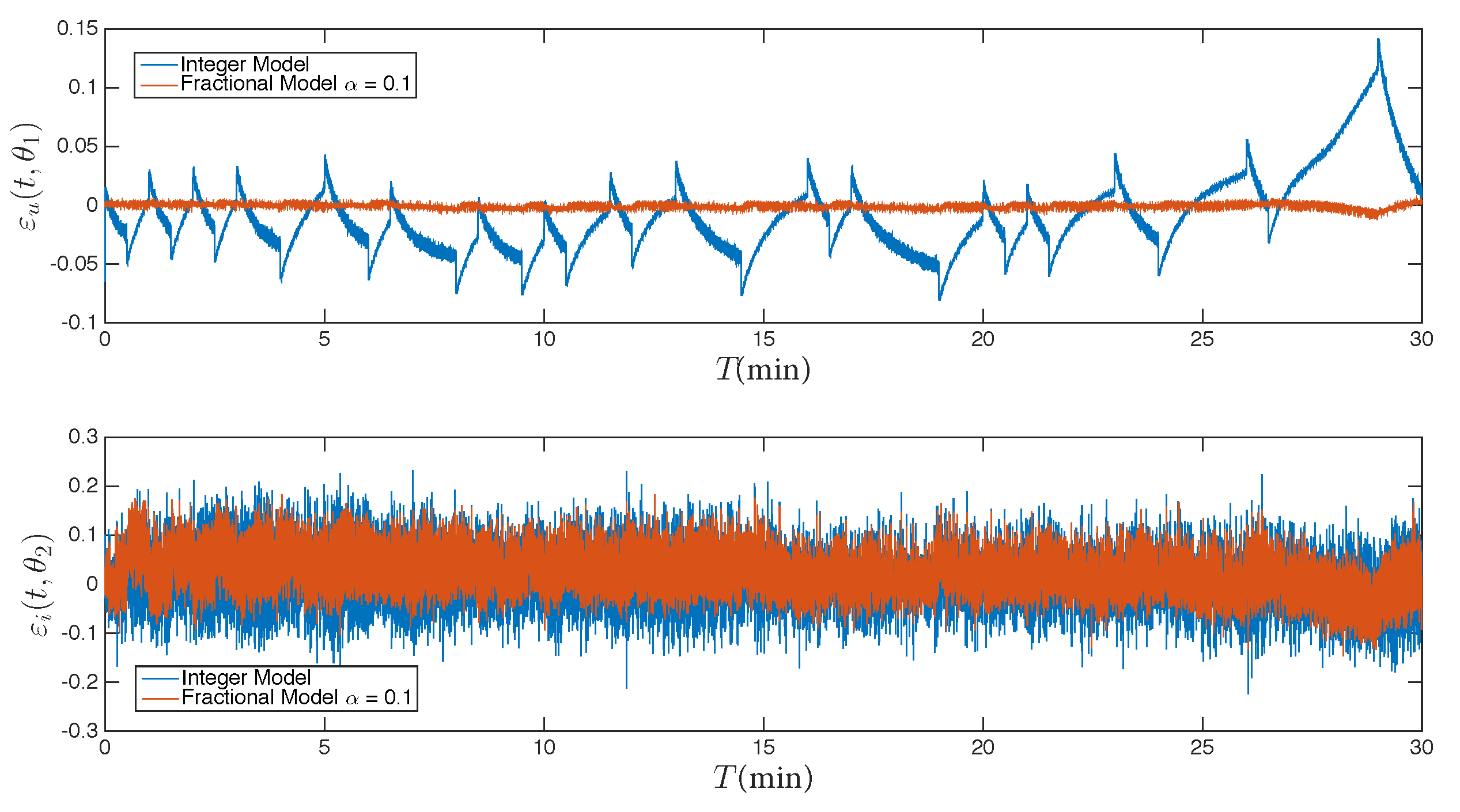
Model Fit Ratio	Fractional Model	Integer Model
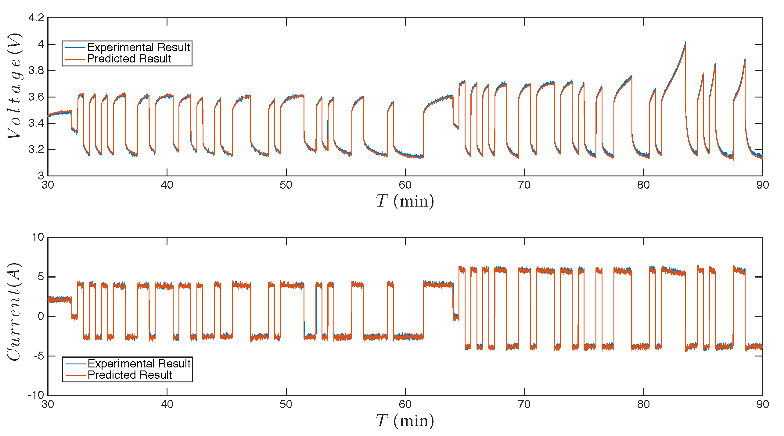
Voltage Model ${\mathsf{\gamma }}_v$	98.9893%	81.7168%
Current Model ${\mathsf{\gamma }}_i$	97.5721%	97.1509%
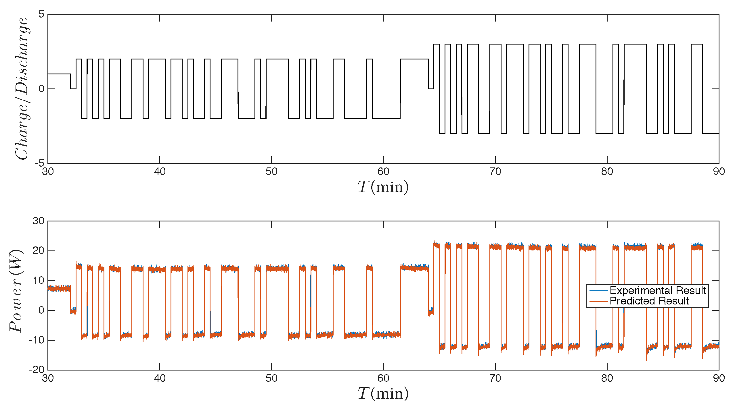
Power Storage/Delivery Model ${\mathsf{\gamma }}_p$	97.9440%	91.0754%

, the model fit ratios comparison illustrates that our proposed fractional models via the LSSVF method obtain more accurate estimation for all of the voltage models, the current model and the power storage/delivery model, assuming that fractional models are more believable than integer models.

Furthermore, the last 60 min data set is used to validate the estimated voltage model and the current model in Equations (24) and (30), respectively. The comparison of the predicted and measured results is shown in Figure 11. The comparison results indicate that the estimated models can also capture the dynamics of the objective system in the last 60 min and predict well with various C-rate charging and discharging and the wider range of SOC. As indicated in Figure 12, the predicted power output, which is combined by the product of the predicted voltage and current, is compared with measured power. The results validate that our proposed dynamic model can accurately predict the dynamics from the demand signal to the power storage/delivery signal of the battery for various operating situations of the battery.

5. Conclusions

System identification of a proposed FDM of a battery via the LSSVF method is described in this paper. This method allows for a consistent estimation of the battery output dynamics by fixing the value of the fractional differential order and then computing smooth fractional derivative signals of voltage and current signals to perform parameter estimation through standard Least Squares minimization. Furthermore, an additional line search over the fractional differential order is utilized to minimize the estimation error and find the best fractional differential order. The proposed method is applied to model the dynamics from a power demand signal to the actual power storage/delivery of a LiFePO${}_4$ battery cell. This is done by estimating two separate FDMs from the power demand signal to the voltage and current signals measured at the battery in real-time. Based on the experimental data set obtained from the LiFePO${}_4$ battery system, comparison of predicted and measured results validates that the FDM estimated via the LSSVF method can capture the power storage/delivery dynamics over a large operation range of the battery and reveal better prediction performance than standard linear differential equation models with integer derivatives. It is anticipated that the proposed estimation method is easily implemented in a BMS to determine and predict the power delivery dynamics of a battery.

References

- Kanchev, H.; Lu, D.; Colas, F.; Lazarov, V.; Francois, B. Energy Management and Operational Planning of a Microgrid with a PV-Based Active Generator for Smart Grid Applications. IEEE Trans. Ind. Electron. 2011, 58, 4583–4592. [Google Scholar] [CrossRef] [Green Version]
- Chaturvedi, N.A.; Klein, R.; Christensen, J.; Ahmed, J.; Kojic, A. Algorithms for Advanced Battery-Management Systems. IEEE Control Syst. 2010, 30, 49–68. [Google Scholar] [CrossRef]
- Perez, H.; Shahmohammadhamedani, N.; Moura, S. Enhanced Performance of Li-Ion Batteries via Modified Reference Governors and Electrochemical Models. IEEE/ASME Trans. Mechatron. 2015, 20, 1511–1520. [Google Scholar] [CrossRef]
- Guo, X.; Kang, L.; Yao, Y.; Huang, Z.; Li, W. Joint Estimation of the Electric Vehicle Power Battery State of Charge Based on the Least Squares Method and the Kalman Filter Algorithm. Energies 2016, 9, 100. [Google Scholar] [CrossRef]
- Lee, J.; Sung, W.; Choi, J.H. Metamodel for Efficient Estimation of Capacity-Fade Uncertainty in Li-Ion Batteries for Electric Vehicles. Energies 2015, 8, 5538–5554. [Google Scholar] [CrossRef]
- Hua, Y.; Xu, M.; Li, M.; Ma, C.; Zhao, C. Estimation of State of Charge for Two Types of Lithium-Ion Batteries by Nonlinear Predictive Filter for Electric Vehicles. Energies 2015, 8, 3556–3577. [Google Scholar] [CrossRef]
- Zou, Z.; Xu, J.; Mi, C.; Cao, B.; Chen, Z. Evaluation of Model Based State of Charge Estimation Methods for Lithium-Ion Batteries. Energies 2014, 7, 5065–5082. [Google Scholar] [CrossRef]
- Sidhu, A.; Izadian, A.; Anwar, S. Adaptive Nonlinear Model-Based Fault Diagnosis of Li-Ion Batteries. IEEE Trans. Ind. Electron. 2015, 62, 1002–1011. [Google Scholar] [CrossRef]
- Xing, Y.; Ma, E.W.M.; Tsui, K.L.; Pecht, M. Battery Management Systems in Electric and Hybrid Vehicles. Energies 2011, 4, 1840–1857. [Google Scholar] [CrossRef]
- Lee, Y.S.; Cheng, M.W. Intelligent control battery equalization for series connected lithium-ion battery strings. IEEE Trans. Ind. Electron. 2005, 52, 1297–1307. [Google Scholar] [CrossRef]
- Lawder, M.T.; Suthar, B.; Northrop, P.W.C.; De, S.; Hoff, C.M.; Leitermann, O.; Crow, M.L.; Santhanagopalan, S.; Subramanian, V.R. Battery Energy Storage System (BESS) and Battery Management System (BMS) for Grid-Scale Applications. Proc. IEEE 2014, 102, 1014–1030. [Google Scholar] [CrossRef]
- Elsayed, A.T.; Lashway, C.R.; Mohammed, O.A. Advanced Battery Management and Diagnostic System for Smart Grid Infrastructure. IEEE Trans. Smart Grid 2016, 7, 897–905. [Google Scholar] [CrossRef]
- Bruen, T.; Hooper, J.M.; Marco, J.; Gama, M.; Chouchelamane, G.H. Analysis of a Battery Management System (BMS) Control Strategy for Vibration Aged Nickel Manganese Cobalt Oxide (NMC) Lithium-Ion 18650 Battery Cells. Energies 2016, 9, 255. [Google Scholar] [CrossRef]
- Xia, M.; Lai, Q.; Zhong, Y.; Li, C.; Chiang, H.D. Aggregator-Based Interactive Charging Management System for Electric Vehicle Charging. Energies 2016, 9, 159. [Google Scholar] [CrossRef]
- Xia, B.; Wang, H.; Wang, M.; Sun, W.; Xu, Z.; Lai, Y. A New Method for State of Charge Estimation of Lithium-Ion Battery Based on Strong Tracking Cubature Kalman Filter. Energies 2015, 8, 13458–13472. [Google Scholar] [CrossRef]
- Yuan, S.; Wu, H.; Ma, X.; Yin, C. Stability Analysis for Li-Ion Battery Model Parameters and State of Charge Estimation by Measurement Uncertainty Consideration. Energies 2015, 8, 7729–7751. [Google Scholar] [CrossRef]
- Scavongelli, C.; Francesco, F.; Orcioni, S.; Conti, M. Battery management system simulation using SystemC. In Proceedings of the 2015 12th International Workshop on Intelligent Solutions in Embedded Systems (WISES), Ancona, Italy, 29–30 October 2015; pp. 151–156.
- Fang, H.; Zhao, X.; Wang, Y.; Sahinoglu, Z.; Wada, T.; Hara, S.; de Callafon, R.A. Improved adaptive state-of-charge estimation for batteries using a multi-model approach. J. Power Sources 2014, 254, 258–267. [Google Scholar] [CrossRef]
- Moura, S.J.; Chaturvedi, N.A.; Krstic, M. PDE estimation techniques for advanced battery management systems—Part I: SOC estimation. In Proceedings of the 2012 American Control Conference (ACC), Montreal, QC, Canada, 27–29 June 2012; pp. 559–565.
- Moura, S.J.; Chaturvedi, N.A.; Krstić, M. PDE estimation techniques for advanced battery management systems—Part II: SOH identification. In Proceedings of the 2012 American Control Conference (ACC), Montreal, QC, Canada, 27–29 June 2012; pp. 566–571.
- Shiau, J.K.; Ma, C.W. Li-Ion Battery Charging with a Buck-Boost Power Converter for a Solar Powered Battery Management System. Energies 2013, 6, 1669–1699. [Google Scholar] [CrossRef]
- Zhao, X.; de Callafon, R.A. Data-based modeling of a lithium iron phosphate battery as an energy storage and delivery system. In Proceedings of the 2013 IEEE American Control Conference (ACC), Washington, DC, USA, 17–19 June 2013; pp. 1908–1913.
- Mastali, M.; Samadani, E.; Farhad, S.; Fraser, R.; Fowler, M. Three-dimensional Multi-Particle Electrochemical Model of LiFePO4 Cells based on a Resistor Network Methodology. Electrochim. Acta 2016, 190, 574–587. [Google Scholar] [CrossRef]
- Abada, S.; Marlair, G.; Lecocq, A.; Petit, M.; Sauvant-Moynot, V.; Huet, F. Safety focused modeling of lithium-ion batteries: A review. J. Power Sources 2016, 306, 178–192. [Google Scholar] [CrossRef]
- Santhanagopalan, S.; Guo, Q.; Ramadass, P.; White, R.E. Review of models for predicting the cycling performance of lithium ion batteries. J. Power Sources 2006, 156, 620–628. [Google Scholar] [CrossRef]
- Zhang, D.; Popov, B.N.; White, R.E. Modeling Lithium Intercalation of a Single Spinel Particle under Potentiodynamic Control. J. Electrochem. Soc. 2000, 147, 831–838. [Google Scholar] [CrossRef]
- Sepasi, S.; Roose, L.R.; Matsuura, M.M. Extended Kalman Filter with a Fuzzy Method for Accurate Battery Pack State of Charge Estimation. Energies 2015, 8, 5217–5233. [Google Scholar] [CrossRef]
- Rahmoun, A.; Biechl, H. Modelling of Li-ion batteries using equivalent circuit diagrams. Available online: http://pe.org.pl/articles/2012/7b/40.pdf (accessed on 21 July 2016).
- He, H.; Xiong, R.; Fan, J. Evaluation of Lithium-Ion Battery Equivalent Circuit Models for State of Charge Estimation by an Experimental Approach. Energies 2011, 4, 582–598. [Google Scholar] [CrossRef]
- Gao, L.; Liu, S.; Dougal, R.A. Dynamic lithium-ion battery model for system simulation. IEEE Trans. Compon. Packag. Technol. 2002, 25, 495–505. [Google Scholar]
- Klein, R.; Chaturvedi, N.A.; Christensen, J.; Ahmed, J.; Findeisen, R.; Kojic, A. Electrochemical Model Based Observer Design for a Lithium-Ion Battery. IEEE Trans. Control Syst. Technol. 2013, 21, 289–301. [Google Scholar] [CrossRef]
- Eckert, M.; Kolsch, L.; Hohmann, S. Fractional algebraic identification of the distribution of relaxation times of battery cells. In Proceedings of the 2015 54th IEEE Conference on Decision and Control (CDC), Osaka, Janpan, 15–18 December 2015; pp. 2101–2108.
- Malti, R.; Victor, S.; Oustaloup, A.; Garnier, H. An optimal instrumental variable method for continuous-time fractional model identification. IFAC Proc. Vol. 2008, 41, 14379–14384. [Google Scholar] [CrossRef]
- Victor, S.; Malti, R.; Oustaloup, A. Instrumental variable method with optimal fractional differentiation order for continuous-time system identification. IFAC Proc. Vol. 2009, 42, 904–909. [Google Scholar] [CrossRef]
- Diethelm, K. The Analysis of Fractional Differential Equations; Springer Berlin Heidelberg: Berlin/Heidelberg, Germany, 2010. [Google Scholar]
- Kaczorek, T.; Rogowski, K. Fractional Linear Systems and Electrical Circuits, Studies in Systems, Decision and Control; Springer International Publishing: Cham, Switzerland, 2015; Volume 13. [Google Scholar]
- Podlubny, I. The Laplace Transform Method for Linear Differential Equations of the Fractional Order. 1997. arXiv:funct-an/9710005. arXiv.org e-Print archive. Avaliable online: http://arxiv.org/abs/funct-an/9710005 (accessed on 21 July 2016).
- Kexue, L.; Jigen, P. Laplace transform and fractional differential equations. Appl. Math. Lett. 2011, 24, 2019–2023. [Google Scholar] [CrossRef]
- Ljung, L. System Identification. In Signal Analysis and Prediction; Procházka, A., Uhlíř, J., Rayner, P.W.J., Kingsbury, N.G., Eds.; Birkhäuser Boston: Boston, MA, USA, 1998; pp. 163–173. [Google Scholar]
- Cois, O.; Oustaloup, A.; Poinot, T.; Battaglia, J.L. Fractional state variable filter for system identification by fractional model. In Proceedings of the 2001 European Control Conference (ECC), Porto, Portugal, 4–7 September 2001; pp. 2481–2486.
- Garnier, H.; Wang, L.; Young, P.C. Direct Identification of Continuous-Time Models from Sampled Data: Issues, Basic Solutions and Relevance. In Identification of Continuous-time Models from Sampled Data; Garnier, H., Wang, L., Eds.; Springer: London, UK, 2008; pp. 1–29. [Google Scholar]
- Garnier, H.; Gilson, M.; Bastogne, T.; Mensler, M. The CONTSID Toolbox: A Software Support for Data-based Continuous-time Modelling. In Identification of Continuous-time Models from Sampled Data; Garnier, H., Wang, L., Eds.; Springer: London, UK, 2008; pp. 249–290. [Google Scholar]
- Tepljakov, A.; Petlenkov, E.; Belikov, J. FOMCON: Fractional-order modeling and control toolbox for MATLAB. In Proceedings of the 2011 Proceedings of the 18th International Conference Mixed Design of Integrated Circuits and Systems (MIXDES), Gliwice, Poland, 16–18 June 2011; pp. 684–689.