An Algorithmic Game Approach for Demand Side Management in Smart Grid with Distributed Renewable Power Generation and Storage

Abstract

In this paper, the problem of minimizing electricity cost and the peak system load in smart grids with distributed renewable energy resources is studied. Unlike prior research works that either assume all of the jobs are interruptible or power-shiftable, this paper focuses on more challenging scenarios in which jobs are non-interruptible and non-power-shiftable. In addition, as more and more newly-built homes have rooftop solar arrays, it is assumed that all users are equipped with a solar-plus-battery system in this paper. Thus, power can be drawn from the battery as needed to reduce the cost of electricity or to lower the overall system load. With a quadratic load-dependent cost function, this paper first shows that the electricity cost minimization problem in such a setting is NP-hard and presents a distributed demand-side management algorithm, called DDSM, to solve this. Experimental results show that the proposed DDSM algorithm is effective, scalable and converges to a Nash equilibrium in finite rounds.

1. Introduction

The cost of electricity generation in a power grid can vary hour by hour depending on numerous factors, including the type of fuels used, power plants, transmission and distribution lines, weather conditions, regulations and demands. For many decades, economists have argued that retail electricity prices should thus fluctuate to help cut power costs for users with flexible power consumption schedules and to reduce the peak system load [1]. 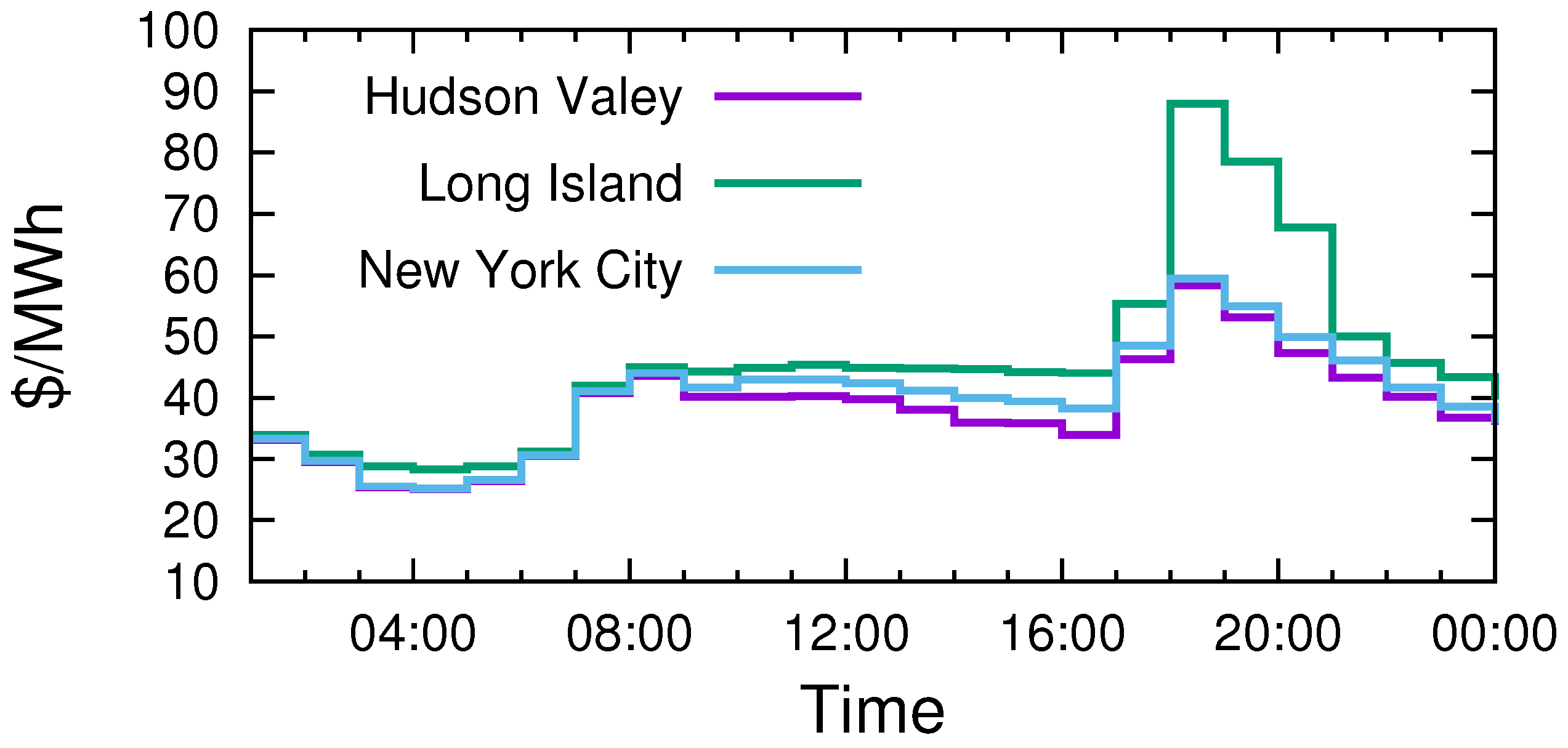Figure 1 shows examples of hourly electricity prices for Hudson Valley, Long Island and New York City on 1 December 2011 [2]. Under the dynamic pricing scheme, electric utility companies provide consumers with information about the actual cost of electricity at any given time via text messages, emails, telephones or smart meters. Consumers, in turn, adjust their electricity usage to coincide with the times that prices are lower. However, they need to closely monitor the price changes in order to take advantage of the lower prices, which is not very practical. Therefore, the first goal of this paper is to design an autonomous scheduling algorithm that can simultaneously minimize electricity costs for all users and the peak system load.

In addition to shifting loads to non-peak hours, energy costs and the peak system demand can be lowered by utilizing ambient energy. In the past few years, there has been an increasing number of grid-connected solar-plus-battery systems installed in the residential market. The City of Lancaster, California, for example, has required newly-built homes to feature solar power systems since 1 January 2014 [3]. Although these distributed renewable power sources are not as reliable as traditional power plants fueled by coal or natural gas, they can be used to further reduce energy costs for users. Hence, the second goal of this paper is to develop a power management algorithm for maximizing the utility of such renewable power systems.

There have been some research studies in the literature addressing similar problems under various settings, such as single-user scenarios [4,5,6], interruptible or power-shiftable appliances (i.e., appliances that are allowed to consume power in an intermittent fashion) [7,8,9], load-independent electricity pricing (i.e., the electricity price does not depend on the overall demand on the entire grid) [5,6,10,11] and centralized renewable power generation [12]. Among the aforementioned studies, References [6,11] are probably the ones that are most similar to ours. However, the authors in [6,11] assume that the electricity prices are independent of the overall system load and are known to the consumers beforehand.

In summary, this paper studies the problem of demand-side management for smart grids with distributed renewable power generation and storage. The focus is on scenarios in which appliances are non-interruptible and non-power-shiftable. Here, non-interruptible means that once an appliance is started, it cannot be interrupted until its task is finished; while non-power-shiftable means that the power consumption pattern of an appliance cannot be arbitrarily adjusted depending on the optimization methods. An example of a non-interruptible device is washing machines. A washing machine is also non-power-shiftable because its power consumption cannot be arbitrarily adjusted and must be strictly followed [13]. Although this paper focuses on the scheduling of non-interruptible appliances, the proposed model and algorithms can be easily extended to handle interruptible appliances, as well. Throughout the paper, it is assumed that each appliance has an associated deadline and that all users are equipped with a renewable power generation and storage system. There is a single electric utility company in the grid. To provide reliable energy, the utility company uses generators that burn fossil fuels. Thus, similar to [8,12,14], the power generation cost is assumed to be a quadratic function of the system load and can vary in real time. Under such a setting, the goals of this paper are reducing the peak system demand, as well as minimizing energy costs for all users. To solve this problem, a bottom-up approach is adopted. First, the complexity of the problem is analyzed. Then, an algorithm inspired by the local search concept is proposed to solve the job scheduling problem. Based on the resulting job schedules, a power management algorithm is developed to reduce the cost of electricity further by drawing power from the battery at time intervals when the electricity prices are high and charging the battery for future use when the electricity prices are low. Lastly, combining the aforementioned job scheduling and power management algorithms, a multi-user distributed algorithm, called DDSM, is proposed to minimize the overall energy costs for all users in the grid. Experimental results show that the DDSM algorithm is effective, scalable and converges in finite rounds.

The rest of this paper is organized as follows. Section 2 reviews related works. Section 3 introduces the system model and the problem formulation. Section 4 presents the proposed algorithms for solving the electricity cost minimization problem. Section 5 analyzes and discusses the experimental results. In the end, Section 6 concludes the paper.

2. Related Works

There have been some research studies that have addressed the problems of minimizing the peak-to-average ratio (PAR) in load demand or electricity costs in smart grids under various settings. Mohsenian-Rad et al. [7] considered the PAR minimization problem in an autonomous power grid in which the utility company can adopt adequate pricing tariffs that differentiate energy usage in terms of both time and level. The price information and the current total load of the system can be exchanged via a communication system between the utility company and the end users. The authors showed that under a common scenario, with a single utility company serving multiple customers, the globally optimal performance can be achieved using an algorithmic game approach. Nguyen et al. [8] extended this earlier work [7] by allowing end users to store purchased electricity in a battery when the system load is low and then draw on the saved energy when the system load is high. The work in [9] extended the idea further by considering the possibility of injecting stored energy back to the grid, although the goal was minimizing the electricity cost rather than minimizing the PAR. Note that all of the aforementioned works adopt a simplified model in which the operations of all household appliances are assumed to be interruptible. In other words, appliances can alternate between active and inactive states as long as they finish their jobs before the given deadlines. In this regard, [15] adopted a more realistic model in which appliances are non-interruptible. The authors proposed a centralized approximation algorithm to solve the PAR minimization problem from the perspective of the utility company. Goudarzi et al. [10] also adopted the non-interruptible load model. However, rather than minimizing the PAR, the authors studied a single-user electricity cost minimization problem. A branch-and-bound-based approach was applied to solve the problem under the time-of-use (time-based pricing is a pricing strategy where the electricity price for any given time is pre-established and known to consumers in advance) pricing model. Samadi et al. [16] considered both interruptible and non-interruptible appliances. The objective was to minimize PAR with real-time pricing. Nonetheless, unlike our models, which allow non-interruptible appliances to be delayed, the authors of [16] assumed that non-interruptible appliances became active right at the earliest time slot in which they could be scheduled. Li et al. [17] considered both interruptible and non-interruptible appliances. Unlike the aforementioned works that directly minimize either the PAR or the electricity cost, the authors modeled demand-side management as a utility maximization game between the utility company and the end users. Similar to [16], there are also a few differences in the way non-interruptible appliances were modeled in [17]. For some non-interruptible appliances, the authors assumed that their working times were given and fixed (e.g., air conditioner), while others were modeled as power-shiftable devices (e.g., hybrid electric vehicles).

As one of the key features of a smart grid is the ability to accommodate all generation and storage options, more and more research studies have started to introduce various types of distributed power generation sources, including renewables. Moon et al. [4] studied a job-shop scheduling problem with time- and machine-dependent electricity costs by considering distributed energy resources (mainly fuel cells) and energy storage. The goal was to minimize the overall electricity cost, as well as the sum of maximal-completion-time related costs for a single production facility. The work in [6] considered the problem of minimizing residential electricity bills under the time-of-use pricing tariff. Each residential house was assumed to have a photovoltaic system and an energy storage system. To prevent all of the appliances from converging to time slots with low electricity prices, Yu et al. [6] introduced a constraint to limit the peak system load. Under the assumption that the hourly energy generation of the photovoltaic system is known, Yu et al. [6] utilized some optimization software package to solve the problem. The work in [12] focused on minimizing the electricity cost for an isolated micro-grid with one wind turbine, one fast responding conventional generator and several users. The authors used a Markov chain with six states to model the stochastic wind power generation process and proposed an optimal consumption strategy based on the backward induction technique. The problem setting in [6] is probably the most similar to that considered here. However, this paper focuses on non-interruptible and non-power-shiftable loads with real-time pricing, which makes the problem more challenging.

Apart from job scheduling, some research studies have also considered the possibility of reducing energy costs by carefully scheduling conventional power generators, such as [11,18]. The authors of [18] studied an electricity generation cost minimization problem for micro-grids equipped with both unstable renewable sources and conventional power generators. The goal was to determine a robust schedule for the appliances and the conventional generators under uncertain renewable sources. To deal with the uncertainty of renewable sources, the authors developed a novel uncertainty model to capture the randomnesses of renewable energy generation. In general, the authors assumed that the distribution of renewable energy generation is shifting around a known distribution that can be obtained either by prediction or long-term field measurements. Then, based on the aforementioned assumption, a robust optimization problem was formulated. To allow an easier solution, the authors decomposed the prime problem into a main problem and a subproblem. The subproblem was solved first to estimate the renewable power generation. Then, the result was fed to the main problem to determine the optimal schedule for the appliances and the conventional generators. The authors of [11] extended [18] to deal with cases in which the electricity price is also uncertain. Since the solution approach is similar to that of [18], we refer the reader to [11] for details. In this paper, although it is assumed that the distribution of uncertain renewable energy is known for the sake of clarity, our proposed method can be combined with robust optimization techniques, such as the primal cut algorithm in [19], to solve the electricity cost minimization problem when the real distribution of uncertain renewable is not available. More details on this are discussed in Section 4.5.

3. System Model

In this paper, a slotted time system is adopted. The time during a day is partitioned into T slots. Each user i has a set of appliances $A_i$, and each appliance $a_{ij}\in A_i$ has an energy consumption profile $(e_{ij},d_{ij})$, where $e_{ij}$ and $d_{ij}$ are the per-time slot power consumption and the time-to-completion of $a_{ij}$, respectively. Moreover, every appliance $a_{ij}$ has a deadline ${\beta }_{ij}$ specified by the user. For example, a user can set the deadline of her washer-dryer to 8 a.m. to make sure clean clothes are readily available before leaving for work. Let $s_{ij}(t)$ denote a binary variable indicating whether appliance $a_{ij}$ starts at time slot t. Then, the deadline constraint can be formulated as:

$$\sum _{t=1}^{{\beta }_{ij}-d_{ij}+1}{s}_{ij}(t)=1$$

(1)

Equation (1) implies that an appliance $a_{ij}$ must start at a time slot that is sufficiently ahead of its deadline, so that its task can be completed in time. During each active time slot, an appliance $a_{ij}$ must consume $e_{ij}$ amount of energy. This can be expressed as:

$$E_{ij}(t)=e_{ij}·I_{ij}(t)$$

(2)

where:

$$I_{ij}(t)=\sum _{k=max\{1,t-d_{ij}+1\}}^t{s}_{ij}(k)$$

(3)

is an indicator function that is equal to one if $a_{ij}$ is active at time t and is equal to zero otherwise.

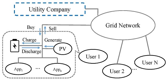
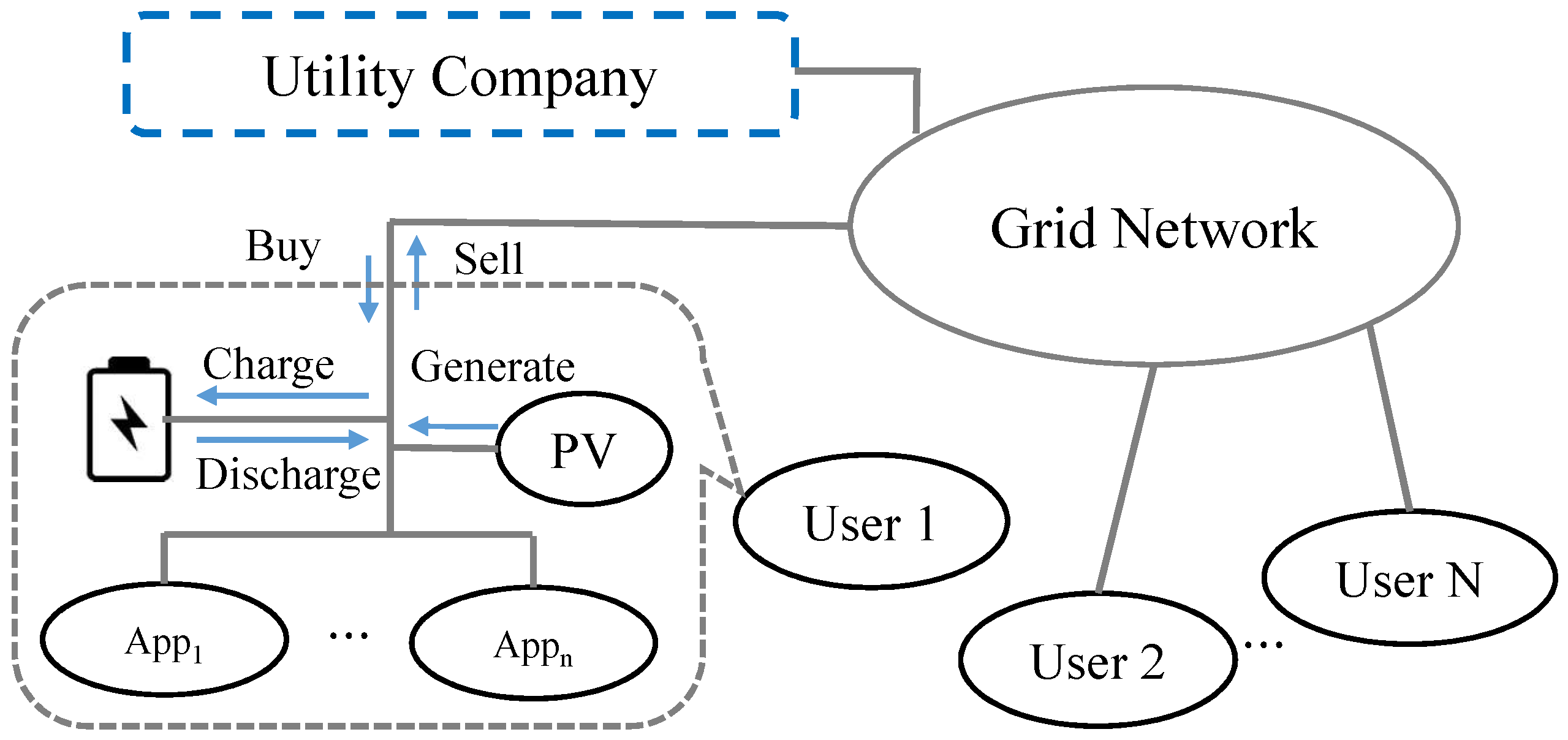
As shown in Figure 2, it is assumed that each user has an ambient energy-harvesting device and a side battery in our model. The ambient energy harvested at a specific time slot $r_i(t)$ can be either used to fulfill the user’s demands, saved into the battery for later use, or injected back into the grid to lower the aggregate system load. Let $r_i^d(t)$, $r_i^b(t)$ and $r_i^g(t)$ denote these three portions of $r_i(t)$, respectively. Then, the following equality must hold:

$$r_i(t)=r_i^d(t)+r_i^b(t)+r_i^g(t)$$

(4)

In addition to renewable energy, a user can also draw power from the grid and the battery to fulfill his or her demands. Thus, the following energy balance constraint must be satisfied at all times:

$$\sum _{j\in A_i}{E}_{ij}(t)\le g_i^d(t)+{\eta }_d·b_i^d(t)+r_i^d(t)$$

(5)

In Equation (5), $g_i^d(t)$ and $b_i^d(t)$ denote the amount of energy drawn from the grid and the battery to support the operations of user i’s appliances, respectively; and ${\eta }_d$ is the battery discharge efficiency. Regarding charge and discharge, a user’s battery level $b_i(t)$ varies over time as follows:

$$b_i(t+1)=b_i(t)-b_i^d(t)-b_i^g(t)+{\eta }_c·(r_i^b(t)+g_i^b(t))$$

(6)

where $b_i^g(t)$ denotes the amount of energy drawn from the battery that is injected back into the grid and ${\eta }_c$ is the battery charge efficiency. As a battery cannot be in charging and discharging states simultaneously, the following constraints are introduced to prevent that from happening [20]:

$$\begin{array}{c}\hfill r_i^b(t)+g_i^b(t)\le M·I_i^b(t)\end{array}$$

(7)

$$\begin{array}{c}\hfill b_i^d(t)+b_i^g(t)\le M·(1-I_i^b(t))\end{array}$$

(8)

where $I_i^b(t)$ is a binary variable indicating whether user i’s battery is in the charging state at time t and M is a constant big number. Next, to ensure that there is always backup power for emergency use, the battery levels of all users are required to be maintained at or above their initial levels at the end of the scheduling horizon:

$$b_i(0)\le b_i(T)$$

(9)

where $b_i(0)$ is the initial battery level. Lastly, a battery’s level can never go beyond the maximum capacity or drop below zero. Therefore:

$$0\le b_i(t)\le B_i$$

(10)

Define $L_i(t)=g_i^d(t)+g_i^b(t)-{\eta }_d·b_i^g(t)-r_i^g(t)$ to be the load imposed on the power grid by user i at time t. The total conventional power $L(t)$ that needs to be generated at each time slot is therefore:

$$L(t)=\sum _{i\in N}{L}_i(t)=\sum _{i\in N}\left\{g_i^d(t)+g_i^b(t)-{\eta }_d·b_i^g(t)-r_i^g(t)\right\}$$

(11)

Similar to [8,12,14], the total power generation cost $C(x)$ is assumed to be quadratic and non-decreasing. In algebra, a quadratic function is a polynomial of degree two, such as:

$$C(x)=a{x}^2+b$$

(12)

Similar to [8], an average cost-based pricing scheme is considered in this paper. Given the aggregate load of the system $L(t)$ at time slot t, the energy provider sets the retail electricity price for time slot t as:

$$P(t)=\frac{C(L(t))}{L(t)}$$

(13)

Users share the power generation cost based on their load proportions. In other words, the electricity cost $C_i(t)$ for each user i at a specific time slot t is:

$$C_i(t)=L_i(t)\times P(t)=\frac{L_i(t)}{L(t)}C(L(t))$$

(14)

In this setting, our goal is to minimize the overall expected electricity cost for all users:

$$\underset{\mathit{s},\mathit{r},\mathit{b},\mathit{g}}{min}\mathbb{E}\left(\sum _{t=1}^T\sum _{i\in N}{C}_i(t)\right)$$

(15)

Note, in Equation (15), $\mathit{s}=\{s_{ij}(t)|\forall i\in N\wedge a_{ij}\in A_i\wedge 1\le t\le T\}$ denotes the set of appliance scheduling decision variables; $\mathit{r}=\{r_i^d(t)|\forall i\in N\wedge 1\le t\le T\}\cup \{r_i^b(t)|\forall i\in N\wedge 1\le t\le T\}\cup \{r_i^g(t)|\forall i\in N\wedge 1\le t\le T\}$ denotes the set of renewable power management decision variables; $\mathit{b}=\{b_i^d(t)|\forall i\in N\wedge 1\le t\le T\}\cup \{b_i^g(t)|\forall i\in N\wedge 1\le t\le T\}$ denotes the set of battery management decision variables; and $\mathit{g}=\{g_i^d(t)|\forall i\in N\wedge 1\le t\le T\}\cup \{g_i^b(t)|\forall i\in N\wedge 1\le t\le T\}$ denotes the set of grid power management decision variables for all users. The key notations used in the paper are summarized in

Table 1. Parameters.

Symbol	Definition
$B_i$	The capacity of user i’s battery
M	A constant big number
T	The total number of time slots
$d_{ij}$	The number of time slots required by appliance $a_{ij}$ to complete its task
$e_{ij}$	Per-time slot power consumption of appliance $a_{ij}$
$r_i(t)$	The amount of ambient energy harvested by user i at time t
${\eta }_c$	Battery charge efficiency
${\eta }_d$	Battery discharge efficiency

,

Table 2. Variables.

Symbol	Definition
$E_{ij}(t)$	The power consumption of appliance $a_{ij}$ at time t
$I_i^b(t)$	A binary variable indicating whether user i’s battery is in the charging state at time t
$L_i(t)$	The load imposed on the power grid by user i at time t
$L(t)$	The total conventional power that needs generating (also known as the aggregate system load) at time t
$b_i(t)$	The battery level of user i at time t
$s_{ij}(t)$	A binary variable indicating if appliance $a_{ij}$ starts at time slot t
$b_i^d(t)$	The amount of energy drawn from the battery that is used to fulfill the demand of user i at time t
$b_i^g(t)$	The amount of energy drawn from the battery that is injected back into the grid by user i at time t
$g_i^b(t)$	The amount of power drawn from the grid that is saved to the battery for later use by user i at time t
$g_i^d(t)$	The amount of power drawn from the grid that is used to fulfill the demand of user i at time t
$r_i^d(t)$	The portion of harvested ambient energy that is used to fulfill the demand of user i at time t
$r_i^b(t)$	The portion of harvested ambient energy that is saved to the battery for later use for user i at time t
$r_i^g(t)$	The portion of harvested ambient energy that is injected back into the grid by user i at time t

and

Table 3. Sets.

Symbol	Definition
N	The set of users
$A_i$	$A_i=\{a_{i1},a_{i2},\cdots \}$ is the set of appliances of user i
${\mathit{s}}_{\mathit{i}}$	${\mathit{s}}_{\mathit{i}}=\{s_{ij}(t)|a_{ij}\in A_i\wedge 1\le t\le T\}$ is the set of appliance scheduling variables of user i
${\mathit{r}}_{\mathit{i}}$	${\mathit{r}}_{\mathit{i}}=\{r_i^d(t)|1\le t\le T\}\cup \{r_i^b(t)|1\le t\le T\}\cup \{r_i^g(t)|1\le t\le T\}$ denotes the set renewable power management decision variables for user i
${\mathit{b}}_{\mathit{i}}$	${\mathit{b}}_{\mathit{i}}=\{b_i^d(t)|1\le t\le T\}\cup \{b_i^g(t)|1\le t\le T\}$ denotes the set battery management decision variables for user i
${\mathit{g}}_{\mathit{i}}$	${\mathit{g}}_{\mathit{i}}=\{g_i^d(t)|1\le t\le T\}\cup \{g_i^b(t)|1\le t\le T\}$ denotes the set of grid power management decision variables for user i
$\mathit{s}$	$\mathit{s}={\displaystyle \bigcup _{i\in N}}{\mathit{s}}_{\mathit{i}}$ is the set of appliance scheduling decision variables for all users
$\mathit{r}$	$\mathit{r}={\displaystyle \bigcup _{i\in N}}{\mathit{r}}_{\mathit{i}}$ is the set of renewable power management decision variables for all users
$\mathit{b}$	$\mathit{b}={\displaystyle \bigcup _{i\in N}}{\mathit{b}}_{\mathit{i}}$ is the set of battery management decision variables for all users
$\mathit{g}$	$\mathit{g}={\displaystyle \bigcup _{i\in N}}{\mathit{g}}_{\mathit{i}}$ is the set of grid power management decision variables for all users
$\mathit{q}$	$\mathit{q}=\mathit{r}\cup \mathit{b}\cup \mathit{g}$ denotes the union of all power management decision variables for all users

for reference.

4. Distributed Demand-Side Management

If the $L(t)$ term in Equation (14) is expanded, it becomes:

$$\begin{array}{c}\hfill C_i(t)=\frac{L_i(t)}{{\displaystyle \sum _{j\in N}}{L}_j(t)}C(\sum _{k\in N}{L}_k(t))\end{array}$$

(16)

It can be clearly seen that the electricity cost of a user not only depends on his or her own power consumption profile, but also on those of other users. Let $\mathit{q}=\mathit{r}\cup \mathit{b}\cup \mathit{g}$ denote the union of all power management decision variables for all users. Our goal is to find an appliance scheduling strategy, as well as a power management strategy for each user such that the following social cost function is minimized:

$$\alpha (\mathit{s},\mathit{q})=\mathbb{E}\left(\sum _{t=1}^T\sum _{i\in N}{C}_i(t)\right)$$

(17)

This naturally leads to the following non-cooperative game:

Players: 

A set of players N

Strategies: 

Each user selects his or her appliance scheduling strategy ${\mathit{s}}_{\mathit{i}}=\{s_{ij}(t)|a_{ij}\in A_i\wedge 1\le t\le T\}$ and power management strategy ${\mathit{q}}_{\mathit{i}}={\mathit{r}}_{\mathit{i}}\cup {\mathit{b}}_{\mathit{i}}\cup {\mathit{g}}_{\mathit{i}}$ to minimize his or her own electricity cost, where ${\mathit{r}}_{\mathit{i}}=\{r_i^d(t)|1\le t\le T\}\cup \{r_i^b(t)|1\le t\le T\}\cup \{r_i^g(t)|1\le t\le T\}$ denotes the set renewable power management decision variables; ${\mathit{b}}_{\mathit{i}}=\{b_i^d(t)|1\le t\le T\}\cup \{b_i^g(t)|1\le t\le T\}$ denotes the set battery management decision variables; and ${\mathit{g}}_{\mathit{i}}=\{g_i^d(t)|1\le t\le T\}\cup \{g_i^b(t)|1\le t\le T\}$ denotes the set of grid power management decision variables for user i, respectively.

Payoff: 

Negative of the private electricity cost for each user $i\in N$:

$$\begin{array}{c}\hfill -{\alpha }_i({\mathit{s}}_{\mathit{i}},{\mathit{q}}_{\mathit{i}};{\mathit{s}}_{-\mathit{i}},{\mathit{q}}_{-\mathit{i}})=-\sum _t{C}_i(t)\end{array}$$

(18)

where ${\mathit{s}}_{-\mathit{i}}={\displaystyle \bigcup _{j\in N\backslash \{i\}}}{\mathit{s}}_{\mathit{j}}$ and $q_{-i}={\displaystyle \bigcup _{j\in N\backslash \{i\}}}{\mathit{q}}_{\mathit{j}}$ are sets containing the appliance scheduling and the power management strategies of all users, excluding user i, respectively.

Note that such a selfish game strategy may not produce a good solution with respect to the social cost and may not even converge. This is because, given the strategies of the others, a user may choose to schedule his or her appliances at time slots with low electricity prices and/or draw power from the battery at time slots with high electricity prices. If multiple users update their strategies simultaneously, it can results in new peak(s) in the overall system load. However, it will be shown in the following sections that, with carefully designed scheduling and power management algorithms, selfish and greedy strategies can still converge in finite rounds to an equilibrium that is satisfactory to all users.

4.1. Analysis of Computational Complexity

Before presenting the solution, the computational complexity of the problem is analyzed, and the result is given in the following theorem.

Theorem 1. 

Under non-decreasing quadratic cost functions, the electricity cost minimization problem (i.e., Equation (15)) is NP-hard even without considering appliances’ deadlines, renewable energy resources and battery capacity-related constraints.

Proof. 

The NP-hardness can be proven by reducing the well-known NP-hard partition problem to a special instance of the electricity cost minimization problem under the aforementioned dynamic pricing model. Given a set of positive integers $S=n_1,...,n_k$, the partition problem is to divide the set S into two subsets, such that the difference between the sum of the elements in the two subsets is minimal [21]. The reduction works as follows. For each integer $n_i\in S$, an appliance is created and its per-time slot power consumption is set to $n_i$. The durations of all of the appliances are set to one, and there are only two time slots in the scheduling horizon. In addition, there are no deadline constraints on the appliances. Because the electricity price function is quadratic and non-decreasing, the optimal solution to this electricity cost minimization problem must partition the appliances into two subsets, such that the difference between their total energy demands is minimal. Obviously, this solution is also the optimal solution of the original partition problem. Thus, if there exists an algorithm that can solve the electricity cost minimization problem in polynomial time, it can also solve the partition problem in polynomial time, which is a contradiction to the fact that the partition problem is NP-hard. This completes the proof. ☐

4.2. Appliance Scheduling Algorithm

Without considering renewable energy and side batteries, Problem (15) is a pure job scheduling problem, which generally can be solved using the branch-and-bound algorithm. However, in cases where the number of users or appliances is large, branch-and-bound-based methods may not be efficient. Thus, an alternative approach is adopted. Our proposed job scheduling algorithm is inspired by the local search algorithm proposed in [22]. As shown in Algorithm 1, the proposed scheduling algorithm begins with generating an arbitrary feasible scheduling strategy (Line 1). Next, it seeks to reduce the electricity cost by performing a local search. Suppose that an appliance $a_{ij}$ is currently scheduled to start at some time slot t and that the corresponding electricity cost is ${\alpha }_{ij}$. The algorithm repeatedly tries to shift its starting time to a later neighboring time slot (i.e., $t+1,t+2,\cdots$) as long as it does not violate $a_{ij}$’s deadline constraint, and its associated electricity cost remains non-increasing (Line 6). When this process stops, it records the time slot $\widehat{t}$ when the search stopped and the corresponding electricity cost ${\widehat{\alpha }}_{ij}$ as if $a_{ij}$ were to be rescheduled to start at time $\widehat{t}$ (Line 7). The algorithm then searches in the opposite direction. In other words, starting from time slot t, it continuously shifts $a_{ij}$’s starting time to the preceding time slot (i.e., $t-1,t-2,\cdots$) as long as the starting time stays greater than or equal to the current time slot and the electricity cost remains non-increasing (Line 8). When this search process stops, it also records the time slot $\overline{t}$ when it stopped and the corresponding electricity cost ${\overline{\alpha }}_{ij}$ as if $a_{ij}$ were to be rescheduled to start at time $\overline{t}$ (Line 9). The algorithm then compares α, ${\widehat{\alpha }}_{ij}$, ${\overline{\alpha }}_{ij}$ and reschedules $a_{ij}$ to the time slot with the minimum cost while closest to time slot t (Lines 10–12). This local search process is repeated for each appliance until the scheduling strategy stops changing. In Section 4.4, the reason why this strategy is convergent and how the convergence property can be utilized to develop a distributed demand-side management algorithm will be discussed.

Algorithm 1: Appliance scheduling algorithm (executed by each individual user i).

4.3. Power Management

Once the schedule of a user’s appliances is determined (i.e., the values of $s_{ij}(t),\forall t,a_{ij}\in A_i$ are set), the next question is how to further reduce electricity costs for all users by utilizing renewable resources. This problem is stochastic because the amount of available renewable energy at each time slot is dynamic in nature. Similar to [14] and for the ease of explanation and clarity, it is assumed that the joint probability distribution of renewable energy over the whole sequence of future time periods (i.e., $\{P(r_i(t),t=1,\cdots ,T)\}$) is known, and the problem is modeled as a $(T+1)$-stage dynamic program. Cases in which the distribution of renewable energy resources is unknown are discussed later in Section 4.5.

At each time slot, the battery level $b_i(t)$ is used as the system state, and $r_i^d(t)$, $r_i^b(t)$, $r_i^g(t)$, $b_i^d(t)$, $b_i^g(t)$, $g_i^d(t)$ and $g_i^b(t)$ are used as the control variables. The system dynamic is, therefore, linear and time-varying, as specified in Equation (6). Using the backward induction technique, the optimal-value function at each time slot can be defined as:

$$\begin{array}{cc}\hfill {\upsilon }_t(b_i(t))& =\underset{{\mathit{r}}_{\mathit{i}},{\mathit{b}}_{\mathit{i}},{\mathit{g}}_{\mathit{i}}}{min}\mathbb{E}\left(C_i(t)+{\upsilon }_{t+1}(b_i(t+1))\right)\hfill \\ \hfill s.t.& \text{(2), (3), (4), (5), (6), (7), (8), (10), (11), (14)}\hfill \end{array}$$

(19)

where $C_i(t)$ is the electricity cost of user i at time t as defined in Equation (14). The objective of the dynamic program is to find the optimal solution for ${\upsilon }_0(b_i(0))$. To initiate the recursive calculation, the optimal-value function at time slot T (the final stage) must be defined. Recall that one of our goals is to maintain the battery at or above its initial level at the end of the scheduling horizon. Thus, ${\upsilon }_T(b_i(T))$ is defined as:

$${\upsilon }_T(b_i(T))=\left\{\begin{array}{cc}0\hfill & \text{if}{b}_i(T)\ge b_i(0)\hfill \\ \infty \hfill & \text{otherwise}\hfill \end{array}\right.$$

(20)

Solving the dynamic program is of very high complexity because, at every stage, all possible values of the system state, renewable energy levels and their corresponding probabilities must be considered. However, since the joint distribution of $\{P(r_i(t),t=1,\cdots ,T)\}$ is known, one can compute the unconditional expected values of the renewable energy and behave as if they are the (unknown) certain values of the renewable energy for future time periods. This strategy is also adopted by many research studies, such as [14,23]. This transforms the problem into one of dynamic programming under certainty and greatly reduces the computational complexity. Nevertheless, it is important to note that, once the true value of $r_i(t)$ is observed at time $t^{-}$, the expected values of $r_i(t+1),\cdots ,r_i(T)$ will change given the new “initial” condition and the new joint probability distribution. Thus, the dynamic program must be re-evaluated at the beginning of each time slot, and a user only implements the action for the first time period that is indicated as optimal.

The detailed algorithm for solving the dynamic program is presented in Algorithm 2. To begin with, the algorithm works backward in time starting from stage T and calculates all ${\upsilon }_t(b_i(t))$ so that the optimal control at each stage can be determined. When calculating the value of ${\upsilon }_t(b_i(t))$, the values of $C_i(t)+{\upsilon }_{t+1}(b_i(t+1))$ for all $0\le b_i(t+1)\le B_i$ must be evaluated. For each possible value of $b_i(t+1)$, there are three cases to consider. First, if $b_i(t)>b_i(t+1)$, this implies that the battery must be discharged at time t. Therefore, $g_i^b(t)$, $r_i^b(t)$ and $I_i^b(t)$ must be zeros. In addition, since the goal is to minimize the electricity cost, the renewable energy should be used to fulfill the user’s demand first and should only be injected back to the grid when there is any leftover. Thus, $r_i^d(t)=min\{\mathbb{E}(r_i(t)),E_i(t)\}$ and $r_i^g(t)=\mathbb{E}(r_i(t))-r_i^d(t)$, where $\mathbb{E}(r_i(t))$ is the expected value of available renewable energy at time t and $E_i(t)={\displaystyle \sum _{j\in A_i}}{E}_{ij}(t)$ is the total power demand of user i at time t. The same principle applies to the energy drawn from the battery. Define $\Delta =b_i(t)-b_i(t+1)$; then it is clear that $b_i^d(t)=min\{\frac{E_i(t)-r_i^d(t)}{{\eta }_d},\Delta \}$ and $b_i^g(t)=\Delta -b_i^d(t)$. Now, if the renewable energy together with the power drawn from the battery cannot completely fulfill the user’s demand, power must be drawn from the grid. Thus, $g_i^d(t)=E_i(t)-r_i^d(t)-{\eta }_d{b}_i^d(t)$. The second case where $b_i(t)<b_i(t+1)$ and the third case where $b_i(t)=b_i(t+1)$ are very similar; therefore, we refer the readers to Algorithm 2 for details. Once all of the possible values of $C_i(t)+{\upsilon }_{t+1}(b_i(t+1))$ are obtained, the action that results in the minimum ${\upsilon }_t(b_i(t))$ is taken as the optimal control for state $b_i(t)$. This process is repeated until state $b_i(0)$ is reached. Not until then does the algorithm backtrack, and the optimal control actions along the path are taken as the power management strategy for the user.

Algorithm 2: Power management algorithm (executed by each individual user i).

4.4. Distributed Demand-Side Management

Based on the results presented in the previous sections, a distributed demand-side management algorithm called DDSM is proposed for the purpose of minimizing social and private electricity costs. The algorithm is run at the beginning of each time slot. As shown in Algorithm 3, given the current aggregate system load vector $\mathit{L}=[L(t),1\le t\le T]$, a user runs Algorithm 1 to determine a new schedule for the appliances that have not been activated (Line 3). Then, based on the observed renewable energy at the current time slot and the expectations of renewable energy for future time periods, the user applies Algorithm 2 to calculate a new power management strategy (Line 4). After that, the user updates the aggregate system load vector according to his or her new appliance scheduling and power management strategies and sends it to the next user in the grid network (Line 5). This process repeats until convergence. Then, all users apply the actions (activating appliances, drawing power from the grid or batteries, etc.) for the current time slot, as specified in their final convergent strategies (Line 7). It is important to note that all users must take turns executing the DDSM algorithm in order to avoid load synchronization and to ensure convergence. As the DDSM algorithm is run at every time slot, the equilibrium point changes over time. This offers opportunities for all users to adjust their appliance scheduling and power management strategies according to the dynamics of renewable energy. The proof of DDSM’s convergence property is detailed below in Theorem 2.

Algorithm 3: Distributed demand-side management (DDSM) algorithm (executed at the beginning of each time slot).

Theorem 2. 

If the users update their strategies asynchronously, i.e., no two users update their appliance scheduling and power management strategies at the same time, the DDSM algorithm converges in a finite number of rounds.

Proof. 

Recall that Algorithm 1 invoked at Line 3 only shifts the schedule of an appliance if and only if the electricity cost associated with that appliance is non-increasing after the shift. Since the electricity cost is a quadratic and non-decreasing function of the total power demand of the entire grid, this implies that if the total power demands of the entire grid at each time slot are sorted in non-increasing order and put in a vector, this vector will become lexicographically smaller after each shift (given two vectors $x=[x_1,x_2,\cdots ,x_n]$ and $y=[y_1,y_2,\cdots ,y_n]$, it is said $x{\le }_{LEX}y$ if there exists some $0\le i\le n$, such that $\forall 1\le j<i$, $x_j=y_j$ and $x_i<y_i$). Following the same rationale, as the power management strategy generated by Algorithm 2 (invoked at Line 4) is optimal when the uncertain renewable energy at future time slots is replaced by their unconditional expectations, this means that there is no way to reduce the electricity cost at time slots with high electricity prices by drawing power from the battery or the energy-harvesting device. Thus, the power demand vector must also become lexicographically smaller after each run of Line 4. Since this vector of power demands must be lower bounded, as the vector keeps becoming lexicographically smaller and smaller, the DDSM algorithm will eventually converge. This completes the proof. ☐

Based on the arguments in the proof, it can be seen that our proposed appliance scheduling algorithm can still work in cases where an appliance has a non-constant power consumption pattern. However, after each shift of an appliance, not only its associated electricity cost must be non-increasing, the highest aggregate system load during the appliance’s active time slots must also decrease. If the highest aggregate system load does not change, then the second highest system load must decrease, and so on and so forth, in order to ensure convergence.

4.5. Dealing with Uncertain Renewable Energy Resources

In earlier discussions, the probability distribution of renewable energy is assumed to be known for the sake of clarity. However, our proposed algorithms can be combined with robust optimization techniques, such as the primal cut algorithm in [19], to tackle the uncertainty of renewable energy resources. The following paragraphs provide an outline for how to combine the primal cut algorithm with our proposed algorithms to solve the electricity cost minimization problem in cases where the distribution of renewable energy is unknown.

The first step for applying the primal cut algorithm is to formulate the electricity cost minimization problem as a two-stage robust optimization (RO) problem as:

$$\begin{array}{cc}& \underset{\mathit{s}}{min}\underset{u\in U}{max}\underset{\mathit{r},\mathit{b},\mathit{g}}{min}\sum _{t=1}^T\sum _{i\in N}{C}_i(t)\hfill \end{array}$$

(21)

$$\begin{array}{cc}\hfill s.t.& r_i^{(u)}(t)=r_i^d(t)+r_i^b(t)+r_i^g(t)\forall i,t\hfill \\ & \text{(1), (2), (3), (5), (6), (7), (8), (9), (10), (11), (14)}\forall i,t\hfill \end{array}$$

(22)

where U denotes the uncertainty set and $r_i^{(u)}(t)$ denotes the amount of renewable energy available at time t for scenario $u\in U$. Then, the two-stage RO problem is decomposed into a main problem and a subproblem. The subproblem is shown in Equations (23) and (24). The goal of the subproblem is to identify the worst case scenario that incurs the highest minimum electricity cost for a given appliance scheduling strategy for all users (i.e., $s_{ij}(t)$ $\forall a_{ij},t$ are given). Here, a scenario refers to some instance of uncertain renewable energy for the entire scheduling horizon.

$$\begin{array}{cc}& \underset{u\in U}{max}\underset{\mathit{r},\mathit{b},\mathit{g}}{min}\sum _{t=1}^T\sum _{i\in N}{C}_i(t)\hfill \end{array}$$

(23)

$$\begin{array}{cc}\hfill s.t.& r_i^{(u)}(t)=r_i^d(t)+r_i^b(t)+r_i^g(t)\forall i,t\hfill \\ & \text{(2), (3), (5), (6), (7), (8), (9), (10), (11), (14)}\forall i,t\hfill \end{array}$$

(24)

The subproblem may seem difficult to solve as there can be many scenarios to consider. However, as only bad scenarios matter, only a small portion of the uncertainty set needs considering. When examining a particular scenario, Algorithm 2 in Section 4.3 can be applied to compute the optimal power management strategy for all users. Note that, when applying Algorithm 2 to solve the subproblem, all users must take turns running the algorithm until convergence. Once all of the scenarios are examined, the worst case scenario can be identified, and its corresponding electricity cost becomes the lower bound of the original two-stage RO problem, as there might be another appliance scheduling strategy for which the worst-case electricity cost is higher.

For each worst-case scenario identified by the subproblem, the primal cut algorithm generates a set of constraints (i.e., Equations (1)–(14)) and adds these constraints to the main problem. The purpose of the main problem is to identify the appliance scheduling strategy for all users that incurs the maximum minimum electricity cost among those worst-case scenarios identified by the subproblem. Thus, the main problem is formulated as:

$$\begin{array}{cc}& max\psi \hfill \end{array}$$

(25)

$$\begin{array}{cc}\hfill s.t.& \sum _{t=1}^T\sum _{i\in N}{C}_i^{(u)}(t)\ge \psi ,\forall u\in U_w\hfill \\ & \text{(1), (2), (3), (4), (5), (6), (7), (8), (9), (10), (11), (14)}\forall i,t,u\in U_w\hfill \end{array}$$

(26)

In Equation (26), $C_i^{(u)}(t)$ denotes the electricity cost of user i under scenario u at time slot t and $U_w$ denotes the set of worst-case scenarios identified by the subproblem. Solving the main problem can be time consuming because there are many binary variables. To speed up the computation, one can utilize Algorithm 3 in Section 4.4 to compute the optimal appliance scheduling and power management strategies for each scenario $u\in U_w$. 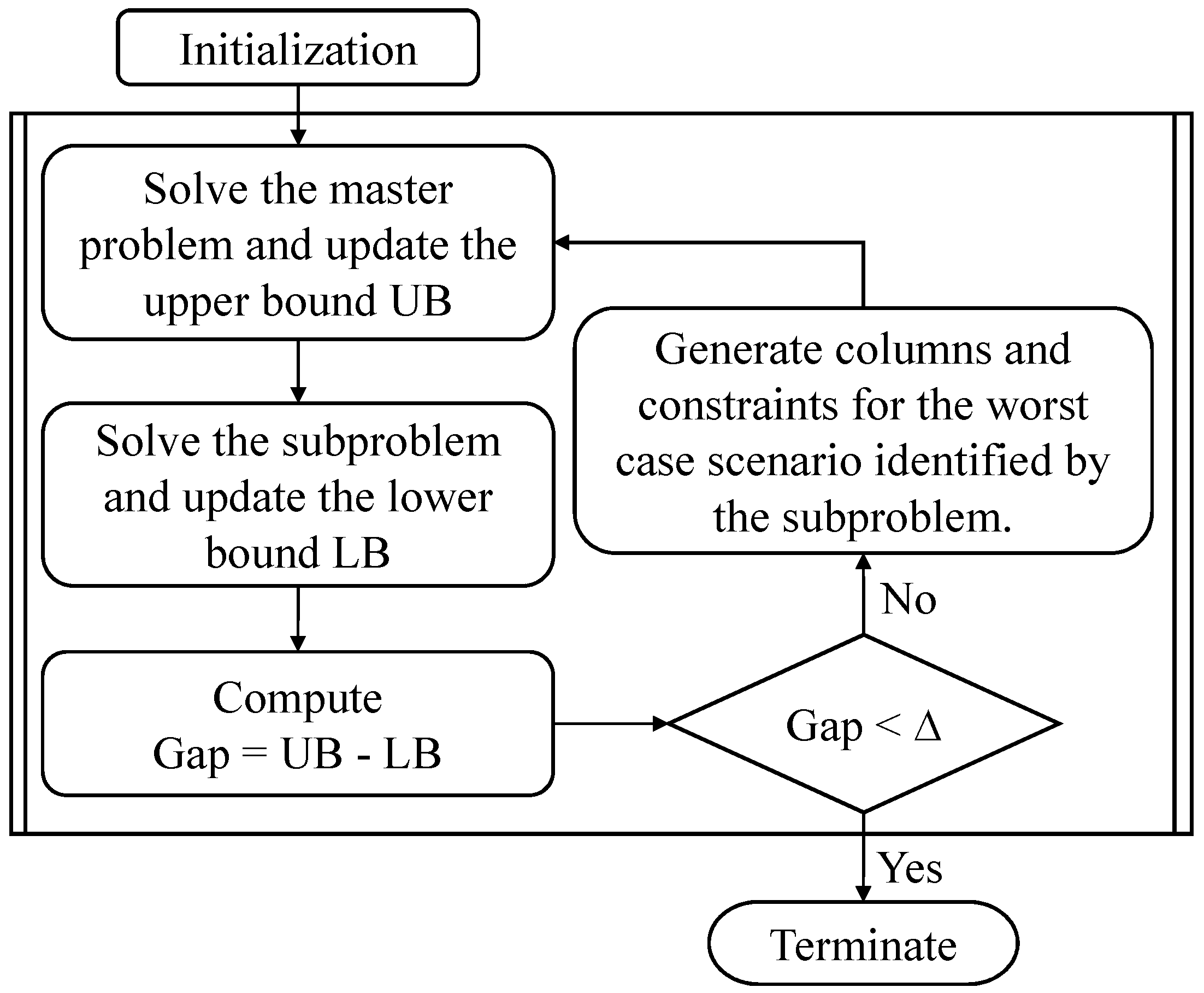In general, the main problem generates an appliance scheduling strategy for each scenario in $U_w$, and the appliance scheduling strategy that incurs the maximum minimum electricity cost is identified and fed to the subproblem for the next round of computation. The objective value of the main problem is an upper bound to the original two-stage RO problem, because the main problem does not consider all of the scenarios. Now, if the gap between the upper bound and the lower bound is smaller than a predefined threshold, the algorithm terminates. Otherwise, the aforementioned steps are repeated until convergence. Due to time and resource constraints, we refer the reader to [19] for more details on the primal cut algorithm and leave the performance analysis for future work. Nonetheless, the steps for the algorithm are summarized in Figure 3 for reference.

5. Evaluation

In this section, the evaluation results of our proposed algorithms are presented and compared to the solutions generated by the DDSM algorithm with those computed by Gurobi [24], which is a commercial mathematical software that solves mixed-integer programming problems using a branch-and-bound-based algorithm. Unless stated otherwise, it is assumed that there are 100 users, each of which has 1–20 jobs with random durations, deadlines and instantaneous power consumption rates. In addition, each user is assumed to have a home photovoltaics system consisting of 20 solar panels of 1.5 m${}^2$ in size with $16.5\%$ power conversion efficiency. Such a system can approximately output 5 kW under the standard test conditions (STC) [25] (the standard test conditions are: normal irradiance of 1000 W/m${}^2$, cell temperature 25 °C (77 °F) and air mass = $1.5$). 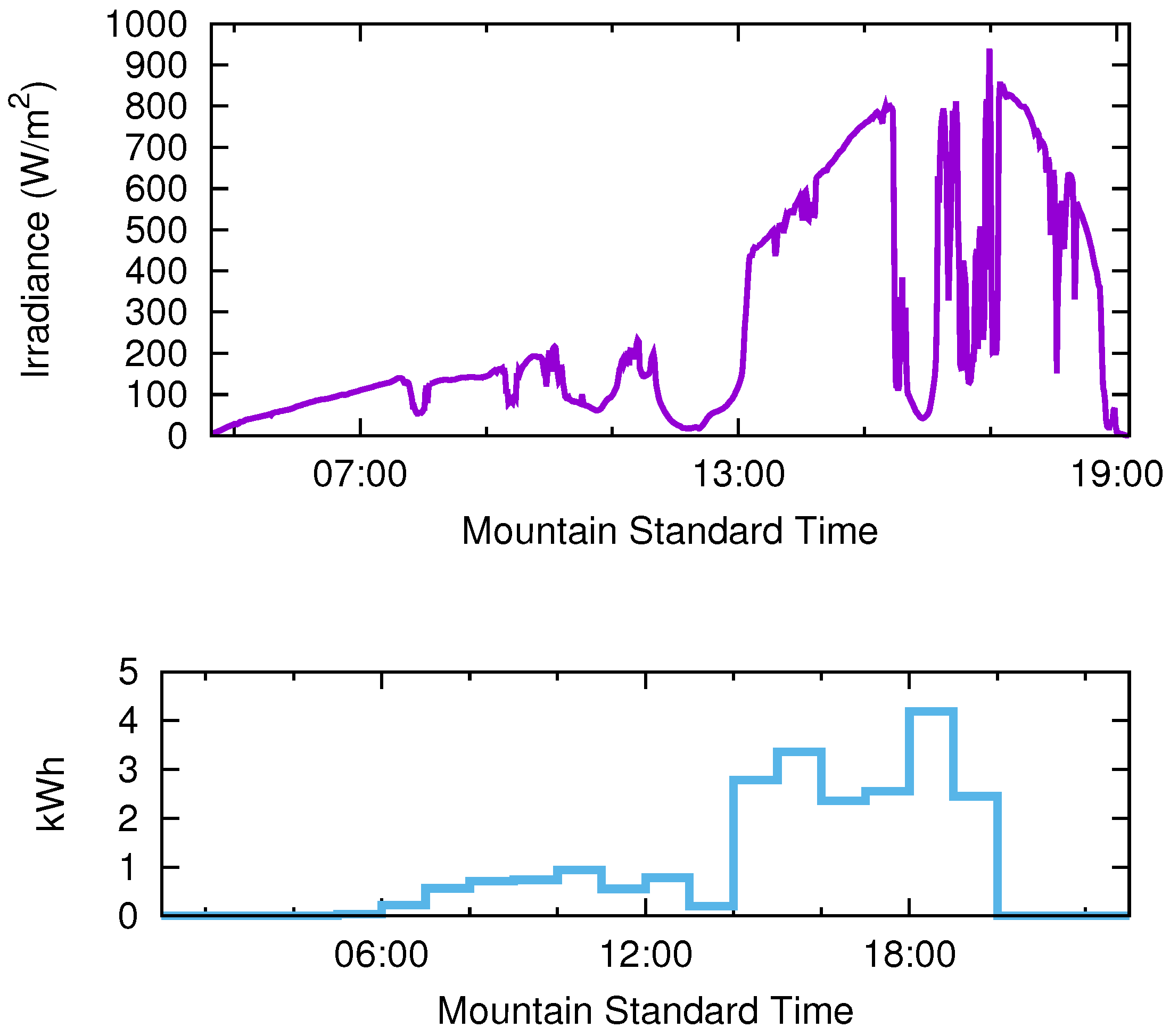The solar system is also assumed to feature a side battery with a capacity 48 V 200 Ah, which is equivalent to 9.6 kWh, for storing excessive energy. Under such assumptions, a renewable energy profile is created for each user using the radiation measurements on 1 June 2015 obtained from the public BMS dataset of the National Renewable Energy Laboratory (shown in Figure 4). The radiation measurements were recorded by a pyranometer mounted on a west-facing surface tilted 90 degrees from the horizontal. The length of the time slots is set to 1 h for convenience. Thus, the amount of available solar energy during a time slot can be easily calculated by taking the average (in kW/m${}^2$) of the solar irradiance for the corresponding hour and multiplying by five. The resulting recharging profile can be found at the bottom of Figure 4. It should be noted that although the length of the time slots is set to 1 h, it can be adjusted as needed. For example, the slot length can be set to 1 min or even 1 s, so as to make the execution time of all appliances a multiple of the slot length. The electricity cost of each time slot is assumed to be $C(L(t))=5\times L{(t)}^2+2$, where $L(t)$ denotes the total power demands at time t. Other detailed experimental parameters are listed in

Table 4. Experimental Parameters.

Parameter	Value
Number of time slots	24
Time slot length	1 h
Number of jobs per user	1–20
Duration of jobs	1–8 slots
Per-time slot power demand of the jobs	1–50 kW
PV system size in kW	5 kW
Battery capacity	48 V 200 Ah
Battery charge/discharge efficiency	0.85 [27]

for reference.

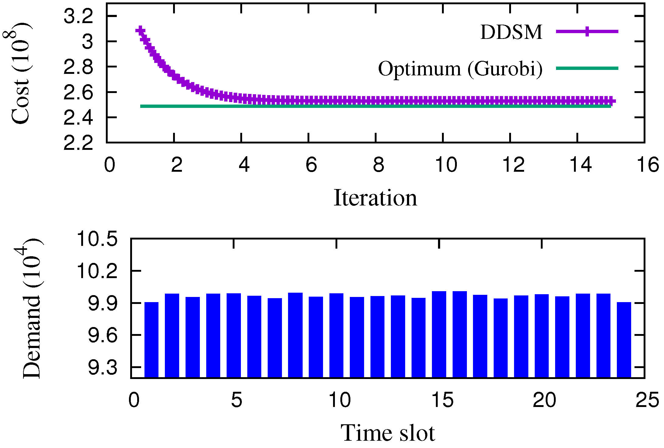
For evaluating our proposed DDSM algorithm, two programs are developed using C++. Given an instance of the electricity cost minimization problem, the first program solves the problem by using the proposed DDSM algorithm, and the other makes use of Gurobi’s API to generate constraints according to the problem specification and solves the optimization problem using a branch-and-bound-based algorithm. First, to show the convergence behavior of the proposed DDSM algorithm, an experiment is conducted to show the social electricity cost for each iteration when the DDSM algorithm is run at the first time slot. Only the result for the first time slot is shown because the rest of the time periods exhibit similar convergence behavior. As can be seen in Figure 5, the DDSM algorithm converges very quickly. The steady state is reached in just five iterations. The final social electricity cost is very close to the optimum computed by the Gurobi solver. It can also be observed in the figure that the planned total power demand of each time slot is smooth with no obvious peak demand periods. This implies that our proposed DDSM algorithm not only can reduce electricity costs for all users, but also can minimize the PAR for the entire grid, which is a win-win solution for both the energy provider and the users.

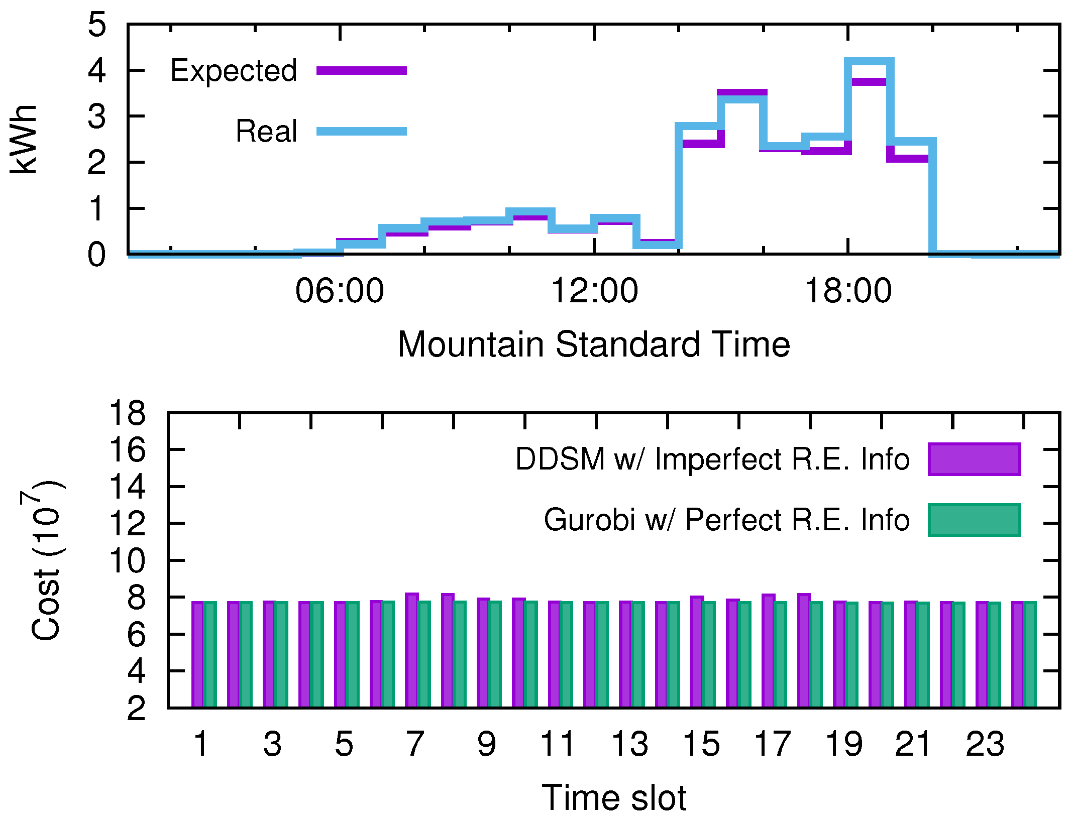
Recall that the DDSM algorithm uses imperfect information regarding the availability of renewable energy when making appliance scheduling and power management decisions for all users. The only piece of information that is available to the DDSM algorithm is the true value of renewable energy observed at the current time slot and the expected values of renewable energy for future time slots. To understand the impact of imperfect information over the performance of the DDSM algorithm, we randomly vary the previously created recharging profile (i.e., the true recharging profile) within the range of $\pm 15\%$ and use it as an estimation of the expected value for renewable energy at each time slot. The result is shown as a purple line on top of Figure 6. The solutions produced by the DDSM algorithm are compared to those computed by Gurobi. When running the DDSM algorithm, the first (true) recharging profile is used to get the value of renewable energy for the current time slot, and the second recharging profile is used to estimate the values of renewable energy for future time slots. In contrast, the Gurobi solver is given the true value of renewable energy for every time slot in the scheduling horizon. Thus, the solution produced by the Gurobi solver is the true optimum. As can be seen at the bottom of Figure 6, the social electricity cost per time slot is very close to the optimum. In the worst case, which happens at Time Slot 17, the electricity cost of the DDSM algorithm is only $5.7\%$ higher than the optimum. This shows that although the DDSM algorithm uses imperfect information of renewable energy when computing appliance scheduling and power management strategies and, thus, its solution may not be as robust as the primal cut algorithm introduced in Section 4.5, it can still achieve reasonable performance.

Next, to evaluate the performance of the DDSM algorithm in terms of optimality and efficiency, the exact information of renewable energy is fed to the DDSM algorithm, and the number of users is varied from 100–1000.

Table 5. Optimality and speed of the DDSM algorithm.

Scenario	Cost		Time (s)
# of Users	DDSM	Gurobi	DDSM	Gurobi
100	$2.50\times {10}^8$	$2.49\times {10}^8$	0.32	10.45
200	$7.48\times {10}^{10}$	$7.42\times {10}^{10}$	1.12	50.13
400	$3.34\times {10}^{11}$	$3.32\times {10}^{11}$	1.73	154
600	$7.89\times {10}^{11}$	$7.87\times {10}^{11}$	3.15	395
800	$1.30\times {10}^{12}$	$1.29\times {10}^{12}$	4.26	826
1000	$2.03\times {10}^{12}$	$2.01\times {10}^{12}$	5.57	1140

shows the solutions produced by the DDSM algorithm and the Gurobi solver and their corresponding computation time for each scenario. As can be seen in the table, the electricity costs incurred by the solutions computed by the DDSM algorithm are all higher than those of the Gurobi solver. However, they are very close, and the electricity costs of the DDSM algorithm are only $0.8\%$ higher than those of the Gurobi solver in the worst case. In addition, as the number of users grows, the amount of time required by the Gurobi solver increases dramatically from $10.45$ s–19 min, while the DDSM algorithm only takes less than 6 s in all scenarios on a PC with a $3.4$-GHz Intel i7 CPU. Although transmission delays are not considered in our experiments and, thus, the time required by the DDSM algorithm may be actually higher in reality, it is still much better in terms of scalability because the number of variables required by the mathematical model will quickly become intractable as the number of users increases. This makes it extremely difficult to solve the problem using off-the-shelf solvers.

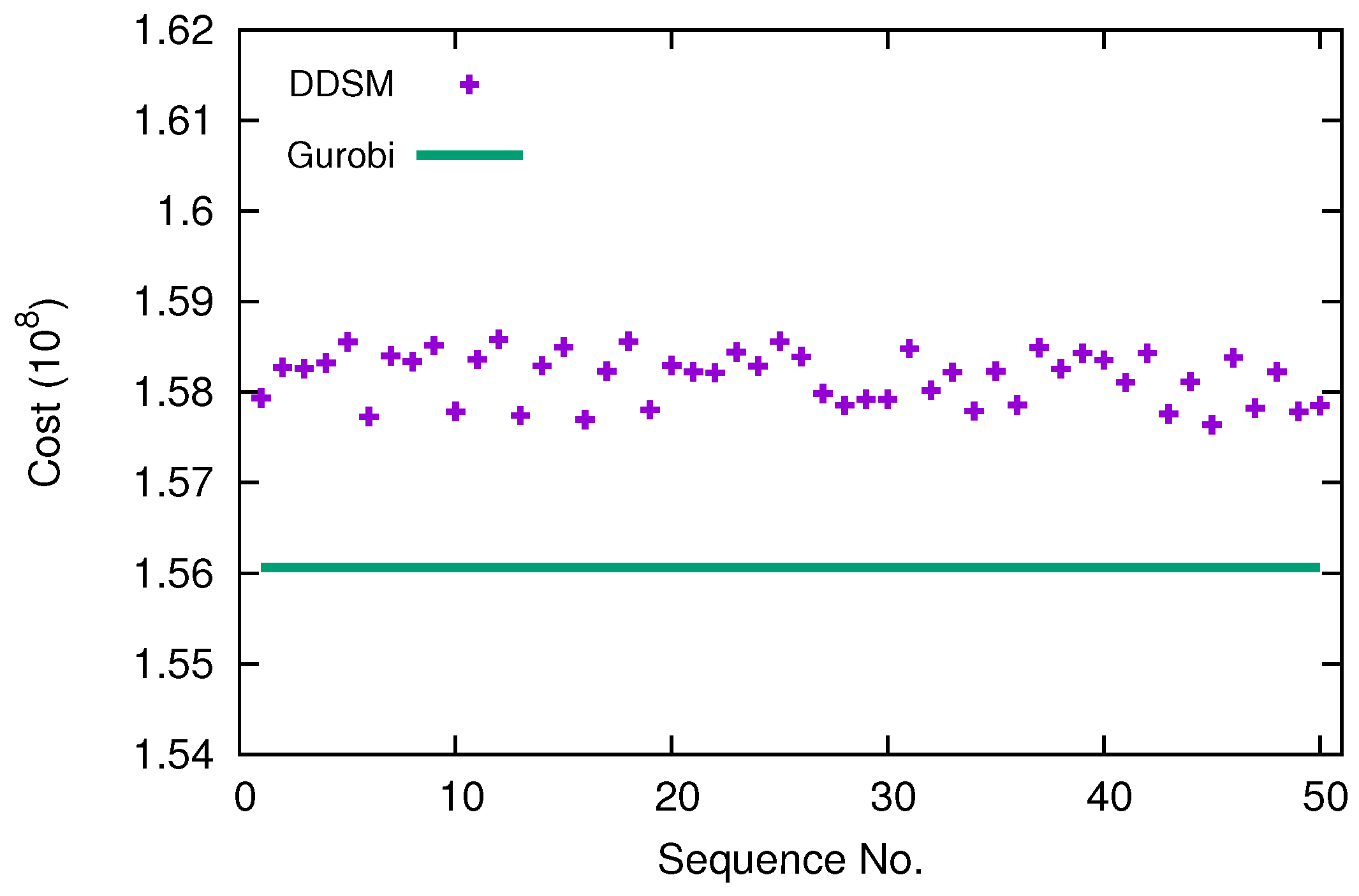
Another factor that may affect the performance of the DDSM algorithm is the order in which the users update their appliance scheduling and power management strategies. This is because the update sequence of the users is essentially the “path” taken by the DDSM algorithm during the optimization process. To see its effects on the performance of the algorithm, 50 random update sequences of users are generated, and the DDSM algorithm is run accordingly to solve the same test case with 100 users, each of which has 1–20 appliances, as described at the beginning of this section. All 50 runs converge, and their corresponding electricity costs are presented in Figure 7. As can be seen in the figure, the update sequence of the users does affect the final solution produced. However, they are all in the vicinity of the optimal solution obtained by Gurobi. This implies that the DDSM algorithm is insensitive to the update sequence of the users, which will allow more flexibility when implementing the DDSM algorithm in a real smart grid network.

Lastly, to show that the proposed DDSM algorithm can work with any number and sizes of time slots, the length of the time slots is varied from 1 h down to 1 min, and the length of the scheduling horizon is kept unchanged at one day. As shown in

Table 6. Performance comparison of different slot sizes.

Scenario	Cost		Time (s)
Slot Size (min)	DDSM	Gurobi	DDSM	Gurobi
60	$2.02\times {10}^8$	$1.99\times {10}^8$	0.107	11.01
30	$3.52\times {10}^8$	$3.46\times {10}^8$	0.218	93.28
10	$1.29\times {10}^9$	$1.27\times {10}^9$	0.325	684.12
1	$9.49\times {10}^8$	—	4.14	—

, the DDSM algorithm is able to produce good solutions in all cases (note, the result of Gurobi for the slot size of 1 min is not included in the table because the solver was not able to give a solution in a reasonable amount of time (one day)). As the number of time slots increases, the computation time of the DDSM algorithm increases slightly, whereas the computation time of Gurobi grows dramatically. This shows the scalability and practicality of our proposed DDSM algorithm over traditional optimization methods.

6. Conclusions

Demand-side management is an important issue for smart grids with distributed renewable power resources. This paper first proposes a single-user job scheduling algorithm and a power management algorithm. Combining the two algorithms, a distributed demand-side management algorithm for minimizing the global electricity cost is developed. Through rigorous analysis and simulations, it is shown that our proposed algorithms are not only efficient and scalable, but are also convergent and very close to the optimum.