Comprehensive Exergy Analysis of Three IGCC Power Plant Configurations with CO₂ Capture

Abstract

We have conducted comprehensive exergy analyses of three integrated gasification combined cycle with carbon capture and storage (IGCC-CCS) power plant configurations: (1) a baseline model using Selexol™ for H₂S/CO₂ removal; (2) a modified version that adds a H₂-selective membrane before the Selexol™ acid gas removal system; and (3) a modified baseline version that uses a CO₂-selective membrane before the Selexol™ acid gas removal system. While holding the coal input flow rate and the CO₂ captured flow rates constant, it was determined that the H₂-selective membrane case had a higher net power output (584 MW) compared to the baseline (564 MW) and compared to the CO₂-selective membrane case (550 MW). Interestingly, the CO₂-selective membrane case destroyed the least amount of exergy within the power plant (967 MW), compared with the Baseline case (999 MW) and the H₂-membrane case (972 MW). The main problem with the CO₂-selective membrane case was the large amount of H₂ (48 MW worth of H₂ chemical exergy) remaining within the supercritical CO₂ that exits the power plant. Regardless of the CO₂ capture process used, the majority of the exergy destruction occurred in the gasifier (305 MW) and gas turbine (~380 MW) subsystems, suggesting that these two areas should be key areas of focus of future improvements.

1. Introduction

Global demand for electricity has been increasing and likely will continue to increase, especially as new and existing technologies are adopted globally. The problem is not the consumption of electricity per se, but rather the environmental impact associated with producing electricity, such as particulate, heavy metal, acid gas, and greenhouse gas emissions. For example, increased greenhouse gas emissions have changed the Earth’s natural atmospheric concentrations. With rising global temperatures and sea levels due to rising greenhouse gas concentrations in the atmosphere, there is a crucial need for eliminating greenhouse gas emissions from fossil-fueled combustion in order prevent future environmental and economic damage [1]. In August of 2015, the U.S. Environmental Protection Agency (EPA) finalized the “Clean Power Plan”, which aims to cut carbon emissions thirty percent from what they were in 2005 by 2030 [2]. This plan determines emission standards for pre-existing power plants [3] and sets a limit of 636 kg (gross) of CO₂ emissions per MWh from new coal-based power plants, averaged over the lifetime of the power plant [4].

In the United States, coal power plants are major generators of both electricity and greenhouse gas emissions, representing both 39% of total power produced and 76% of total CO₂ emissions from electricity generation nationwide [5,6]. Coal power plants are typically one of the two following processes: pulverized coal (PC) or integrated gasification combined cycle (IGCC) power plants. In the first type, the coal is pulverized and then combusted in a boiler to produce steam that is used to generate electricity in a Rankine-only cycle. In an IGCC power plant, however, the coal is first gasified to produce a H₂-and-CO-rich synthetic fuel gas, called syngas, and then this syngas is combusted in a gas turbine to generated electricity. Heat taken from both the syngas and the flue gas is also recovered to produce steam for additional electricity generation. This process is called a Brayton-Rankine (B-R) cycle or sometimes simply called a combined cycle (CC). IGCC power plants are typically associated with higher efficiencies than PC power plants, in part because the efficiency of combusting fuel in combined B-R cycles is higher than in Rankine-only cycles [7]. When equipped with carbon capture and storage (CCS) processes, a PC power plant is expected to obtain a higher heating value (HHV) efficiency of around 26%, whereas an IGCC power plant is expected to obtain a HHV efficiency of 32% or higher with technologies currently in development [8]. An advantage of removing CO₂ from syngas over flue gas is that the partial pressures of CO₂ in a pre-combustion fuel stream is roughly 200× higher than in a post-combustion flue gas stream. A related advantage of pre-combustion CO₂ removal is the greater physical contrast between CO₂ and H₂ molecules than CO₂ and N₂ molecules. The large partial pressure of CO₂ and the large contrast between CO₂ and H₂ allows one to use a physical solvent, such as Selexol™ [9], which has good H₂S/CO₂ selectivity, very good CO₂/H₂ selectivity, and good kinetics for CO₂ absorption/release. Because of the potential for higher net electrical efficiency for a new build, we have chosen here to analyze IGCC-CCS rather than PC-CCS power plants. Though, we recognize that there are many more PC power plants in existence globally, and we recognize that there are good reasons to study CO₂ capture at both PC and IGCC power plants if we are to meaningfully reduce global CO₂ emissions.

Numerous previous authors have analyzed IGCC-CCS power plants from an energy, an exergy and/or an economic perspective. Some particularly useful reports on this subject are the U.S. DOE’s National Energy Technology Laboratory (NETL) Bituminous Baseline Reports, which give a detailed breakdown of the electrical efficiency and levelized cost of electricity of PC, PC-CCS, IGCC, and IGCC-CCS power plants using similar assumptions in all cases [10]. In the latest NETL Bituminous Baseline Report with IGCC & IGCC-CCS configurations [10], the GE-gasifier based IGCC power plant is reported to have an HHV electrical efficiency of 39.0% and the GE-gasifier based IGCC-CCS power plant is reported to have an HHV electrical efficiency of 32.6%. Another useful source for a detailed breakdown of the electricity generation and economics of PC, PC-CCS, IGCC, and IGCC-CCS power plants is the Integrated Environmental Control Model (IECM) by Dr. Edward Rubin’s research group at Carnegie Mellon University [11]. In IECM v9.1, the GE-gasifier based IGCC power plant has an HHV electrical efficiency of 36.4% and the GE-gasifier based IGCC-CCS power plant has an HHV electrical efficiency of 30.8% [12]. One general economic conclusion regarding IGCC-CCS power plants from both NETL reports and IECM is that the cost of the CO₂ capture and compression equipment is quite small compared with the other capital costs at the plant, such as the gasifier and the power cycle equipment. This means that the main economic effect of adding CO₂ capture and compression equipment to the IGCC power plant is the decrease in net overall power production.

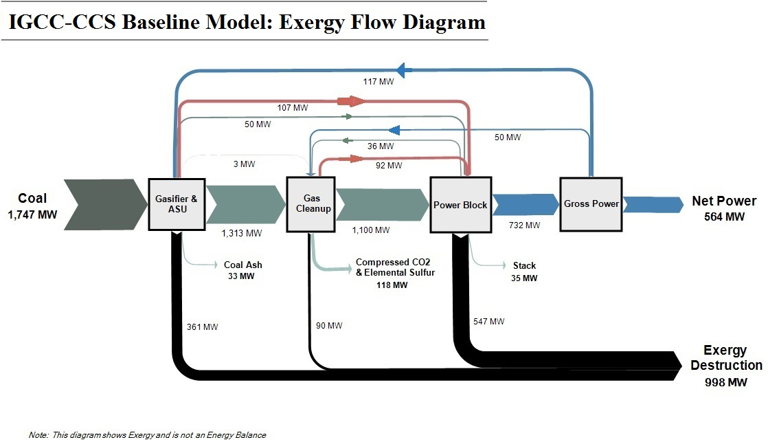
As discussed previously, there is a net power decrease of approximately 6 basis points when adding CO₂ capture and compression. Most of this net power reduction is due to the fairly high exergy in the CO₂ stream leaving the power plant in the CO₂ storage pipeline (15 MPa), whose pressure is significantly higher than both the partial pressure of the CO₂ in the environment (40 Pa) and the partial pressure of CO₂ in the flue gas stream from a coal power plant (15 kPa.) For example, our results later in this paper find that the exergy in the supercritical CO₂ leaving in the CO₂ pipeline is approximately 5% of the exergy in the inlet coal. The remaining power reduction when adding CCS is due to irreversibility within the subsystems that must be added to the power plant, such as the Water-Gas-Shift subsystem and CO₂ capture/compression subsystems. For example, Li et al. [13] conducted an exergy analysis of an IGCC-CCS power plant and found that exergy destruction in the WGS reactor can be quite large when CO conversion rate above 90% are required.

Given this net power reduction, there have been attempts to improve IGCC-CCS power plants so that the net power from an IGCC-CCS power plant is closer to that of an IGCC power plant without CO₂ capture. For example, to improve both net power and overall economics, Franz et al. [14] analyzed the use of porous ceramic membranes and a water-gas shift membrane reactor in comparison to a baseline model using the Selexol™ process. The IGCC baseline in Franz et al. [14] has a net power of 47.4% without CCS. Their Selexol-only IGCC-CCS baseline had an efficiency of 37.1%. Their IGCC configuration with a H₂-selective ceramic membrane after the WGS subsystem had an efficiency of 37.1%. Finally, their IGCC configuration with a H₂-selective ceramic membrane within the WGS subsystem had an efficiency of 41.6%. While the efficiencies of all of their configurations are higher than those of equivalent NETL & IECM models, their relative conclusions are likely still valid because it appears that the reason for the slightly higher starting efficiencies than in NETL and IECM models of an IGCC power plant is due to slightly higher assumptions for the efficiency of heat exchangers, pumps and turbines in the Rankine cycle.

In a similar attempt to improve the efficiency of an IGCC-CCS power plant, Gray et al. [15] presented research on the effect of advanced technologies on both the electrical efficiency and the overall economics of IGCC-CCS configurations. They found that, through a combination of various advanced technologies, the electrical efficiency of an IGCC-CCS power plant could be increased from approximately 31% (reference case) to approximately 40% and that the total plant cost (in $/kW) could be decreased by roughly 40% compared with their reference IGCC-CCS case. The bulk of the gain in efficiency and decrease in total capital cost was from using (a) a high temperature H₂-selective membrane and (b) an advanced turbine designed to operate on H₂ rather than CH₄.

Merkel et al. [16] also studied the use of membranes in CCS. They stated that, while polymeric membranes have a lower hydrogen permeance and selectivity compared to palladium-based membranes, the advantages of polymeric membranes are that they are stable, inexpensive, and easily scaled-up. Krishnan et al. [17] investigated high-temperature polybenzimidazole (PBI) membranes to be used in CCS. They stated that PBI membranes possess “excellent chemical resistance, a very high glass transition temperature (450 °C), good mechanical properties and excellent material processing ability” [17]. Both sets of researchers listed above found that IGCC-CCS configurations with polymeric membranes increased the HHV electrical efficiency compared to their Selexol™ baseline IGCC-CCS cases. The general conclusion from all of the above papers is that H₂-selective membranes can increase the net electrical output and decrease the normalized capital costs (in $/kW.)

Our goal here is not to conduct an economic analysis with a cost comparison between different CO₂ capture technologies. Instead, our main focus here is conducting detailed exergy analyses of three cases in order to help build an understanding of where are the major sources of exergy destruction in the three cases. Our goal here is to present detailed, thorough, and transparent exergy analyses, which builds upon the previous work by authors who have published exergy analyses of IGCC and IGCC-CCS power plants [8,13,18,19,20,21,22,23,24,25]. As such, this paper presents comprehensive exergy analyses on three IGCC-CCS power plants: (a) a baseline model using Selexol™ for H₂S & CO₂ capture; (b) a modified version that incorporates a H₂-selective PBI-membrane operating at 250 °C; and (c) a modified version that incorporates a CO₂ selective membrane. The exergy analyses give crucial insight into understanding where useful work is being wasted and destroyed in each of the subsystems within an IGCC power plant, as well as insight into the exergy remaining in all of the streams exiting the power plant. The exergy analyses presented here are similar to the exergy analyses of IGCC processes conducted by Siefert et al. [8,19]. One difference compared with previous analyses is that we present a detailed exergy analysis of both the baseline and the modified cases. In previous work, we presented the exergy analyses of the modified cases without presenting a full exergy analysis of the baseline model [8,19]. In future work, we will be conducting a full techno-economic analysis of the three cases presented here [26].

2. Exergy Methodology

One way to evaluate the efficiency of a process is to analyze the exergy destruction that occurs throughout the whole process. Exergy is defined as the maximum amount of useful work that can be obtained from a material by bringing it into equilibrium with its environment. This makes exergy a property of both the material and its surroundings. Here, the reference environment was taken to be the Earth’s atmosphere at standard temperature and pressure, 298 K and 1 atm, and with the chemical composition listed in

Table 1. Composition of reference environment at 298 K and 1 atm.

Gas Species	Mol %	Liquid	Activity	Solid	Activity
N2	75.67	H2O(l)	1	CaCO3	1
O2	20.35	NaCl(aq)	Not Appl.	CaSO4·2H2O	1
H2O(g)	3.03			SiO2	1
Ar	0.91			Al2O3	1
CO2	0.04			Fe2O3	1

. The further away the material is from equilibrium with the reference environment, the more exergy is associated with the material. By this definition, exergy can only be positive, unless the material is in complete thermal, mechanical, and chemical equilibrium with the reference environment. Since exergy is equal to the theoretical maximum amount of useful work, tracking the exergy destruction is a good indication for which parts or processes within the power plants have the greatest potential to be improved so as to increase net power production. As seen in Table 1, we have assumed for simplicity that the activities of the liquid and solid species are equal to 1, even though these species do form a mixture in the environment and hence have activities less than 1. We made this assumption for liquid water because different power plants will have reference water environments with different levels of salinity; and we made this assumption for solids because the largest error in the calculation of the exergy in the coal ash and coal slag is the uncertainty in the exact crystal state of the solids entering and exiting the gasifier. This error is much larger than the error in assuming that the activity of each solid species is equal to one.

2.1. Exergy Destruction within Each Subsystem

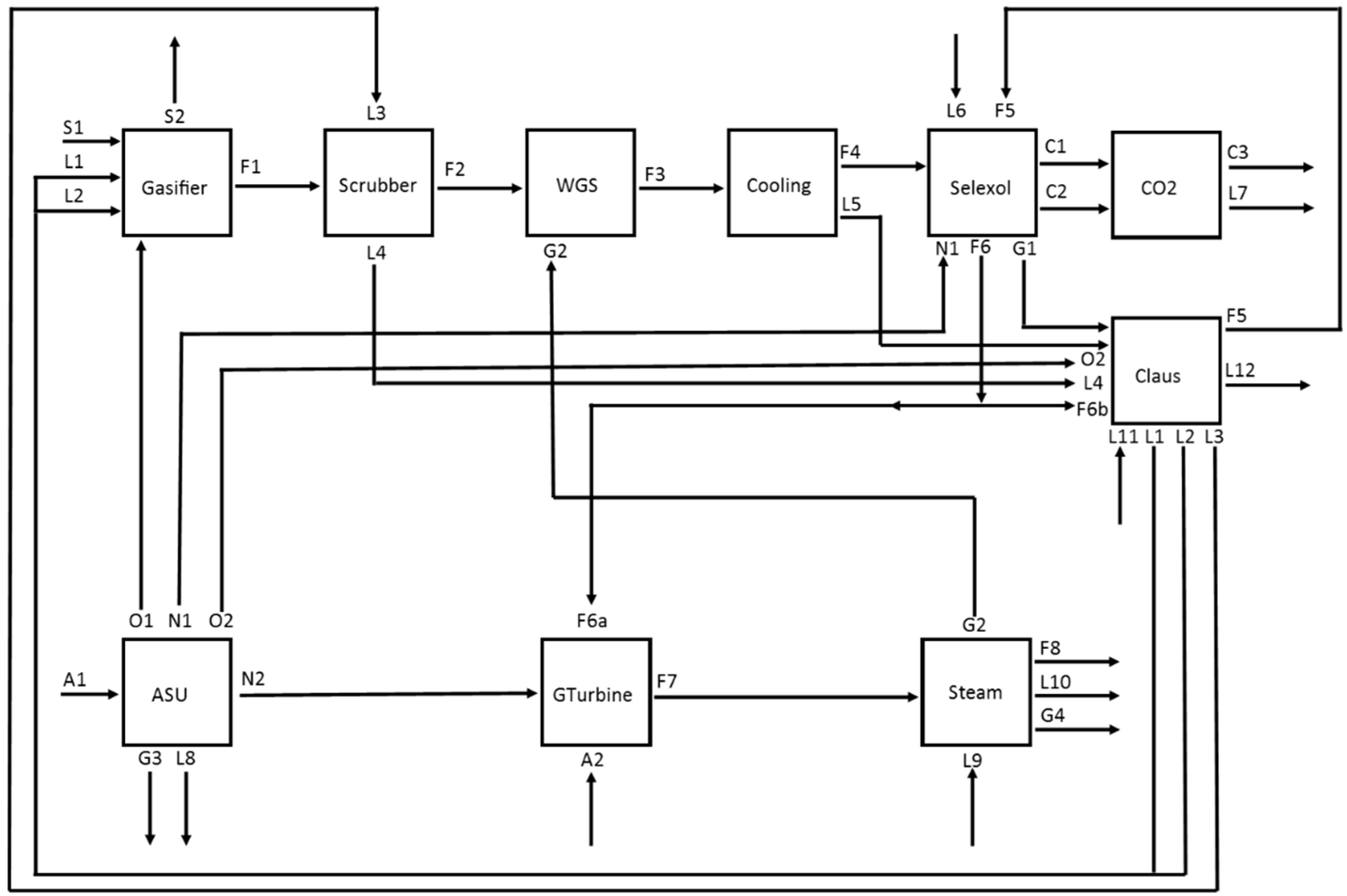
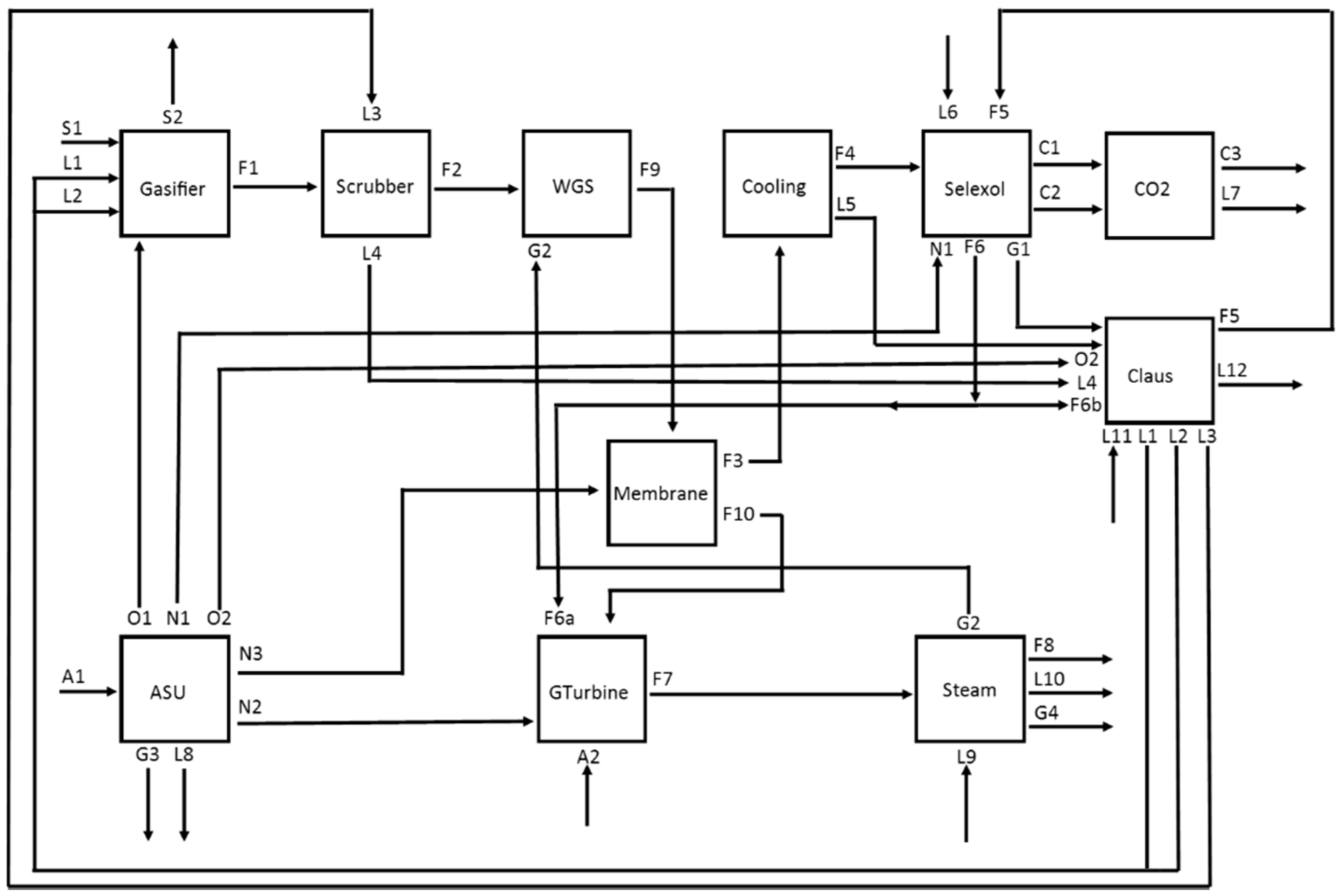
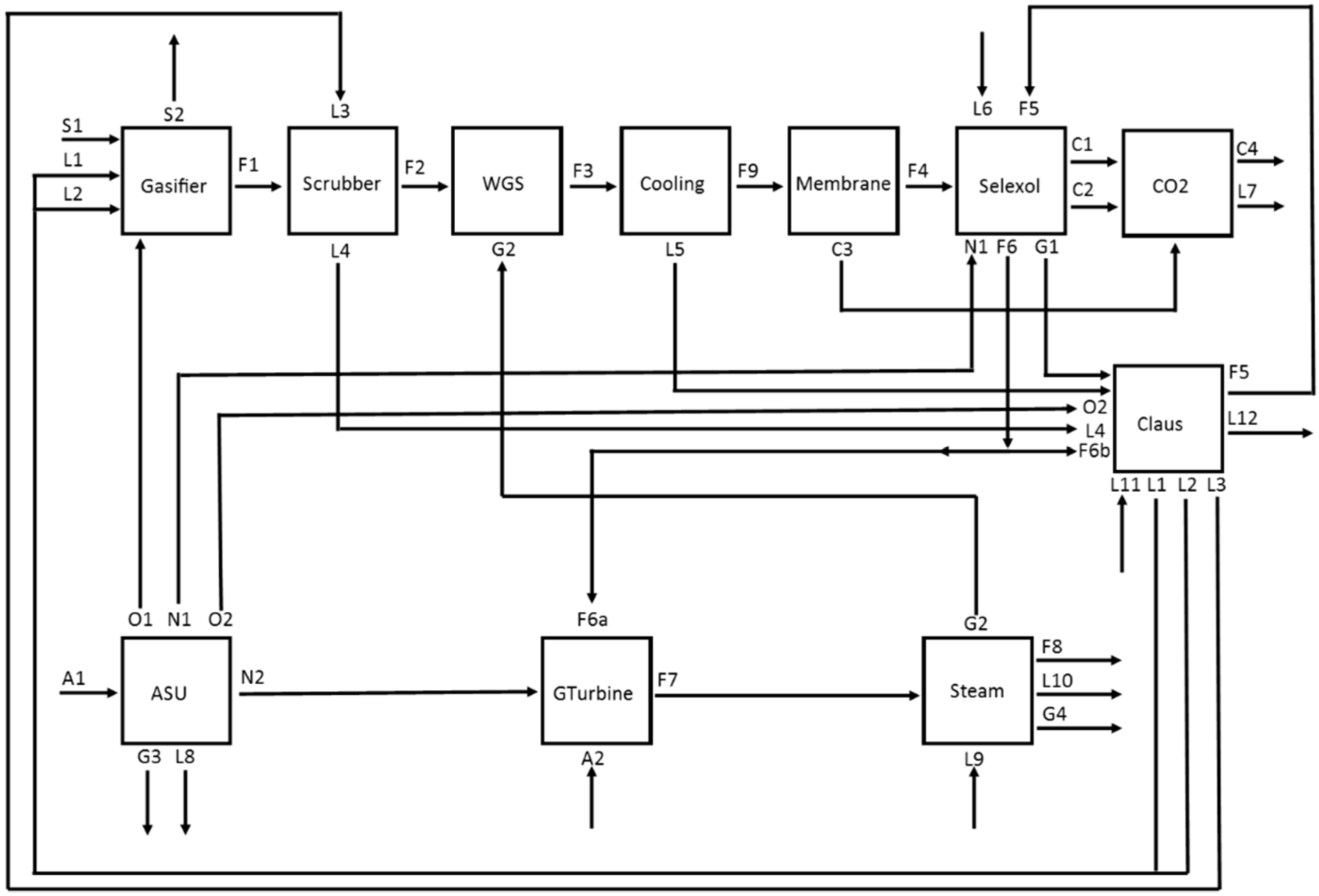
A high-level exergy analysis of an IGCC-CCS power plant was conducted by Kunze et al. [18], in which the overall plant was separated into 3 different subsystems (Gasifier Island, Syngas Treatment, and Combined Cycle.) Here, we break the IGCC-CCS power plant into a total of 10 (or 11) subsystems within the power plant. These 10 (or 11) subsystems can be seen in Figure 1, Figure 2 and Figure 3, each of which will be discussed in more detail in Section 3.1, Section 3.2 and Section 3.3, respectively. All subsystems were assumed to be operating at steady-state conditions. We determined the exergy destruction within each subsystem by taking into account the inlet and outlet streams, the heat entering and leaving, as well as the work being consumed and produced. Since Aspen Plus does not directly calculate the thermal energy sent to the environment, this term was calculated using the First Law of Thermodynamics, as shown in Equation (1).

Equation (1): First Law of Thermodynamics for a steady-state control volume solving for thermal energy transfer to the environment.

$${\dot{Q}}_{env}={\displaystyle \sum }_{i=inlet}{\dot{n}}_i{\widehat{h}}_i-{\displaystyle \sum }_{o=outlet}{\dot{n}}_o{\widehat{h}}_o-\dot{W}-{{\displaystyle \sum }}^{\text{}}{\dot{Q}}_j$$

(1)

where ${\dot{Q}}_{env}$ is the thermal energy sent to the environment, $\dot{n}$ stands for the molar flowrate of streams, $\widehat{h}$ stands for the molar enthalpy of streams, $\dot{W}$ is the electrical work leaving the system, and ${\dot{Q}}_j$ stands for the thermal energy transfer out of (+) or into (−) the subsystem from another subsystem. Diagrams of all of the subsystems for the three models analyzed can be found in the Supplemental Materials, along with a summary of the nomenclature used in this text. The irreversible production of entropy was then calculated using the Second Law of Thermodynamics, taking into account that thermal energy leaves a subsystem at varying temperatures, as shown in Equation (2).

Equation (2): Second Law of Thermodynamics for a steady-state control volume with thermal energy leaving at a range of temperatures.

$${\dot{\sigma }}_{irr}={\displaystyle \sum }_{o=outlet}{\dot{n}}_o{\widehat{s}}_o-{\displaystyle \sum }_{i=inlet}{\dot{n}}_i{\widehat{s}}_i+\frac{{\dot{Q}}_{env}}{T_{env}}+{\displaystyle \sum }_j\frac{{\dot{Q}}_j}{T_{j,o}-T_{j,i}}ln\left(\frac{T_{j,o}}{T_{j,i}}\right)$$

(2)

where ${\dot{\sigma }}_{irr}$ represents the irreversible entropy production, $\widehat{s}$ stands for entropy and T stands for the temperature of the heat. As shown in the last two terms in Equation (2), heat was separated into two categories: (1) heat leaving to the environment and (2) heat being transferred between two subsystems. We did this in order to differentiate between heat used elsewhere in the plant and heat exiting to the environment, the latter of which was assumed to have zero exergy because it will eventually come into equilibrium with the environment. Heat being transferred between subsystems, however, has a certain amount of exergy associated with it. Equation (3) describes how to calculate the exergy associated with heat transferred between sub-systems.

Equation (3): Exergy in thermal energy transferred between subsystems.

$${\dot{E}}_j={\dot{Q}}_j·\left[1-\frac{T_{env}}{T_{j,o}-T_{j,i}}ln\left(\frac{T_{j,o}}{T_{j,i}}\right)\right]$$

(3)

where ${\dot{E}}_j$ is the exergy associated with the heat transfer, $T_{j,i}$ is the temperature of the inlet of a stream that gives/receives thermal energy to/from another subsystem, and $T_{j,o}$ is the temperature of the outlet of such a stream. It should be noted that Equation (3) as well as the last term in Equation (2) are only valid when the specific heat capacity of the fluid does not significantly vary along the length of the heat exchanger.

When heat is transferred between two subsystems, the Steam subsystem was always involved. The exergy destruction associated with heat transfer was calculated two different ways: (a) always being assigned to the Steam subsystem and (b) being assigned to the respective subsystem transferring thermal energy to/from the Steam subsystem. In case (b), $T_{j,i}$ and $T_{j,o}$ are the temperatures of the inlet and outlet of the streams on the Steam side of the HX. Whereas in case (a), $T_{j,i}$ and $T_{j,o}$ are the temperatures of the inlet and outlet of the streams on the non-Steam side of the HX.

Once the irreversible entropy production within a subsystem is calculated using Equation (2), the exergy destruction within the subsystem can be calculated using the Gouy-Stodola Theorem, which is shown in Equation (4).

Equation (4): Guoy-Stodola Theorem.

$${\dot{\Phi }}_{des}=T_{env}·{\dot{\sigma }}_{irr}$$

(4)

This theorem states that the rate of exergy destroyed within a subsystem, ${\dot{\Phi }}_{des}$, is equivalent to the product of the temperature of the environment and the entropy generation rate due to irreversible processes, ${\dot{\sigma }}_{irr}$, within the subsystem.

2.2. Exergy Entering and Exiting Subsystems

An exergy analysis is more than just a second law analysis. Using only Equations (2) and (4), one cannot conduct a full exergy analysis because these equations do not calculate the exergy of streams entering/exiting the entire power plant. To calculate the exergy of a stream, an Excel workbook was used to carry through a series of calculations. Equation (5) is the equation used to calculate the molar exergy of a material stream entering/exiting a subsystem, assuming the gravitational potential and kinetic exergy are negligible.

Equation (5): Molar exergy of a material stream entering/exiting a subsystem.

$$\widehat{e}=\left[\left(\widehat{h}-{\widehat{h}}_{stp}\right)-T_{env}\left(\widehat{s}-{\widehat{s}}_{stp}\right)\right]+{\widehat{e}}_{chem}$$

(5)

Here, $\widehat{h}$ and $\widehat{s}$ represent the molar enthalpy and molar entropy, respectively, of the stream at the temperature and pressure at which they enter/exit a subsystem while the ${\widehat{h}}_{stp}$ and ${\widehat{s}}_{stp}$ represent the molar enthalpy and molar entropy of the stream if the elements in the stream were at the same temperature and mechanical pressure of the reference environment. ${\widehat{e}}_{chem}$ is the molar chemical exergy, which is related to the Gibbs free energy of a species when brought into full chemical equilibrium with the chemically-stable species in the environment, i.e., N₂, O₂, H₂O, CO₂, CaCO₃, CaSO₄·2H₂O, SiO₂, Al₂O₃, and Fe₂O₃.

As shown in Equation (5), the exergy of a stream has both a thermo-mechanical and a chemical exergy component. The specific chemical exergy at STP of each species used in the analysis is shown in

Table 2. Chemical exergy of species at STP.

Gas Species	Molar Chemical Exergy at STP (kJ/mol)	Solid Species	Molar Chemical Exergy at STP (kJ/mol)
N2(g)	0.69	FeO(s)	125.4
O2(g)	3.97	Fe(s)	367.6
H2O(g)	8.55	C(s)	409.8
Ar(g)	11.7	S(s)/S8(s)	602.7/75.3
CO2(g)	19.4	CaO/MgO	0 *
H2(g)	235.2	Na2O/K2O	0 *
CO(g)	274.6	Fe2O3/SiO2/Al2O3	0 *
NH3(g)	336.7	* = approximation due to uncertain crystal state.
H2S(g)	804.6	Liquid Species
CH4(g)	829.6	H2O(l)	0 #
COS(g)	848.8	# = approximation due to uncertain salinity of env.

, which is similar to the values derived by Szargut, Morris and Stewart [27], but derived independently using standard values of the Gibbs free energy of formation and the composition of the environment as listed in Table 1. It should be noted that most of these values for chemical exergy can also be found in Table A-26 of Moran and Shapiro’s 6th edition of Fundamentals of Engineering Thermodynamics [28]. When a mixture is being analyzed, the chemical exergy can be calculated through a weighted average of the chemical exergy of the individual components based on their respective mole fractions. This is due to the fact that gases in the Earth’s atmosphere can be treated as an ideal gas mixture. For simplicity and because the actual crystal state of these species in the coal ash/slag are unknown, we assume that the following species have zero chemical exergy: SiO₂, Al₂O₃, CaO, MgO, Na₂O, K₂O, and Fe₂O₃. As seen in Table 2, we did assume that FeO and Fe have chemical exergy, as calculated from the Gibbs free energy of the reactions that create Fe₂O₃ from FeO and Fe using oxygen at the partial pressure of the environment. While the crystal state of the SiO₂, Al₂O₃, CaO, MgO, Na₂O, and K₂O in the coal ash does change between the inlet and outlet of the gasifier [29], the effect of this change on exergy calculations is small and was ignored because, unlike Fe₂O₃, no redox reaction occurs for these species.

In addition to using the Gouy-Stodola Theorem to calculate the exergy destruction within a subsystem, one can directly calculate the exergy destruction within a subsystem by calculating the difference between the exergy that enters a subsystem and the exergy that leaves a subsystem. This calculation is shown in Equation (6).

Equation (6): Exergy destruction within a steady-state subsystem.

$${\dot{\Phi }}_{des}={\displaystyle \sum }_{i=inlet}{\dot{n}}_i{\widehat{e}}_i-{\displaystyle \sum }_{o=outlet}{\dot{n}}_o{\widehat{e}}_o-\dot{W}-{\displaystyle \sum }_j{\dot{E}}_j$$

(6)

where ${\dot{E}}_j$ is calculated using Equation (3) and $\widehat{e}$ is calculated using Equation (5).

The two routes for calculating exergy destruction, Equations (4) and (6), were used as checks to see if the values determined were the same. As can be checked for all subsystems (see Supplemental Materials), the normalized exergy destruction as calculated using Equation (4) was within ±0.2% of the value calculated using Equation (6), which leads to high confidence in the values presented for the exergy destruction within the subsystems.

2.3. Exergy of Solid Mixtures

The only solid mixtures analyzed in this process are: (1) the solid coal entering, which is the primary source of exergy; and (2) the slag leaving the Gasifier subsystem. As in Field and Brasington [30], the coal represented in our models is an Illinois#6 bituminous coal with a dry basis HHV of 30.5 MJ·kg⁻¹, which converts into a “with moisture” HHV of 27.1 MJ·kg⁻¹. Important values for these solid species streams are listed in

Table 3. Composition of solid streams.

Description	S1	S2
	Inlet Coal	Exiting Slag
Temperature (K)	333	489
Pressure (Mpa)	7.24	5.5
Flowrate (kg·s−1)	62.20	6.61
Enthalpy (MW)	−119.7	−15.0
Entropy (kW·K−1)	−139.4	23.0
Exergy (MW)	1747.43	32.99
Composition (wt %)
C	63.75	12.56
H	4.50	0.16
O	7.0	0.38
N	1.30	0.00
S	2.55	0.00
Cl	0.30	0.00
Moisture Content (H2O)	11.12	0.00
Total Ash	9.70	86.90
SiO2	3.18	29.92
CaO	1.56	14.69
MgO	0.16	1.54
Al2O3	2.58	24.21
Na2O	0.32	2.99
K2O	0.10	0.91
FeO	0.00	3.05
Fe2O3	1.80	0.11
Fe	0.00	9.48

. The enthalpy, entropy and exergy of the inlet coal were estimated by simulating the coal in AspenPlus as a combination of C₁₂H₁₀O, C₄H₅N, C, S, liquid water and ash species, using the elemental analysis provided by Field and Brasington [30]. The exergy of the inlet coal was estimated to be 28.1 MJ·kg⁻¹, which implies a total exergy in the inlet coal of 1747 MW. Using the HHV values listed above, one can convert the exergy efficiencies presented later in this report into HHV electrical efficiencies by multiplying by 28.1/27.1 (103%). Similar to the inlet coal, the enthalpy, entropy and exergy of the exiting slag were estimated by simulating the slag in AspenPlus as a combination of C₁₂H₁₀O, C, and ash species, leading to an exergy per mass of 5.0 MJ·kg⁻¹ and a total exergy remaining in the coal slag of 33 MW.

3. Cases Analyzed

3.1. Baseline Model

AspenPlus V8.4 (Aspen Technology Inc., Bedford, MA, USA) was used to model three IGCC power plants equipped with carbon capture systems. The baseline model used in this project was obtained from an article titled “Baseline Flowsheet Model for IGCC with Carbon Capture” by Field and Brasington [30], which is referred to as the baseline model throughout this paper because of its similarity to the Baseline IGCC-CCS model (Case B5B-Q) in the NETL Bituminous Baseline report [10]. Field and Brasington’s AspenPlus model is publically-available at the article’s website. Similarly, as supplemental material to this manuscript, we are providing the three AspenPlus models used to simulate the baseline and two membrane cases presented here.

The overall flowsheet for the Baseline Model is shown in Figure 1. In this baseline model, 100% of the syngas goes through the Selexol™ subsystem. This IGCC-CCS model includes ten sub-systems, shown by the square blocks in Figure 1. This IGCC-CCS model kept all of the assumptions, calculations, and specifications implemented by Field and Brasington [31]. The labels for the subsystems in Figure 1 are the same as they appear in their original AspenPlus model. Though, to make the process flow diagrams easier to read, the labels for the streams in Figure 1 have been changed from how they appear in their original AspenPlus model. The AspenPlus names for each stream as well as their descriptions can be found in the Supplemental materials. Overall, there are 6 inlets streams (S1 = coal, A1/A2 = ambient air, L6/L9/L11 = liquid water) and 9 outlet streams (S2 = ash, G4/G3/F8 = Exhaust air, L12 = Sulfur Product, C3 = Compressed CO₂, L7/L8/L10 = Liquid discharge).

3.2. H₂-Selective Membrane Model

The second case analyzed was an IGCC power plant with a hydrogen membrane subsystem added between the WGS and Cooling subsystems. Since AspenPlus does not have a membrane module, we used AspenCustomModeler (ACM) to model both the H₂-selective membrane module and the CO₂-selective membrane module. More details on using ACM to model the membrane modules can be found in Section 4. Figure 2 shows the overall process diagram. Entering this membrane subsystem are two counter-flowing streams: (a) the post-WGS syngas feed stream (F9); and (b) the post-ASU nitrogen sweep stream (N3). The permeate stream from the membrane module (F10) contains H₂, N₂, H₂O as well as lesser amounts of CO and CO₂, and this stream goes to the gas turbine. The retentate stream (F3) contains the remaining H₂, H₂O, CO₂, and other gas species. The retentate goes to the Cooling subsystem before going to the Selexol™ subsystem for removal of CO₂ and H₂S. Note that the counterflowing nature of these stream weren’t shown in Figure 2 in order to make the figure easier to read.

The hydrogen membrane was modeled using permeance and selectivity data measured by Los Alamos National Laboratory (LANL) and reported by Berchtold et al. [31]. Their values for mixed gas selectivity (shown in their Table 1) were: H₂/CO₂ = 48, H₂/CO = 100, H₂/CH₄ = 234, H₂/H₂S = 1289. We used their pure gas selectivity of H₂/N₂ = 233 because no mixed gas data was provided in their Table 1. In addition, we used a value of H₂O/H₂ selective of 3, which was derived from results in wet H₂ streams [32]. We specified that 60% of the H₂ in the feed enters the permeate stream and then calculated the compositions of other species in the permeate based on the ACM membrane model. Therefore the permeate stream contains 60% of the H₂, 84% of the H₂O, 2.6% of the CO₂, and trace amounts of other gas species that enters the Membrane subsystem. It is important to note that less thermal energy goes to the Rankine cycle in this model than in the baseline model because 84% of the water in the syngas ends up going directly to the gas turbine, and only 16% of the water vapor in the syngas ends up condensing in the Cooling subsystem.

Other than adding the H₂-selective membrane, a few other minor changes to the baseline model were made, such as increasing the pressures in the HP, MP, and LP flash tanks in the Selexol™ subsystem due to the increased partial pressure of CO₂ entering the Selexol™ subsystem. Increasing the pressures of the flash tanks ensured that the right amount of CO₂ is released from each of the HP, MP, and LP tanks. The pressures of the flash tanks were increased until the hydrogen remaining in the compressed CO₂ was similar to the amount of hydrogen remaining in the Baseline Model. The modified model kept the following key variables the same: (a) coal inlet flow rate; (b) inlet gas turbine temperature; (c) gas and steam turbine isentropic efficiencies; and (d) the amount of captured and compressed carbon dioxide.

3.3. CO₂-Selective Membrane Model

In the CO₂-selective membrane case, an ACM-based membrane subsystem was added between the Cooling and Selexol™ subsystems. The reason that we placed the CO₂-selective membrane after syngas cooling is that CO₂-selective polymers must rely on high solubility of CO₂ over H₂ in the membrane, which is more likely to occur at low temperatures. The cooled syngas entering the CO₂ membrane subsystem is separated into two streams. The retentate stream is sent through the Selexol™ subsystem for further removal of CO₂ and H₂S, and the permeate stream is sent directly to the CO₂-subsystem for compression to 15 MPa. Figure 3 shows the overall process flow diagram. Since there has been less research into CO₂-selective polymeric membranes than H₂-selective polymeric membranes, we chose an optimistic value of CO₂/H₂ selectivity of 50, which is greater than typical values for CO₂/H₂ selectivity measured so far [16,33,34,35,36], most of which are on the order of 10. In addition, we assumed that the selectivity of CO₂ to all other species was 50. The exception here is the selectivity of CO₂ to water vapor, which was chosen to be 0.5, and which had very little impact on results because the water vapor has mostly been condensed out before the CO₂ selective membrane. As will be shown later in this report, even with these optimistic values of CO₂ selectivity, the CO₂-selective membrane case did not perform as well as the baseline or the H₂-selective membrane case. Therefore, we did not run this model at lower values of selectivity, which would have performed even worse because even more H₂, CO, and H₂S would remain in the compressed CO₂ stream (C4).

3.4. Constant Parameters in All Models

To make fair comparisons between the models, we kept some important input parameters constant. In

Table 4. List of input parameters that remain constant in all three models.

Gas Turbine		Steam		Additional Information
Turbine Inlet	1185 °C	HP Inlet	12.5 MPa	ηpump	75.0%–100%
Turbine Outlet	0.105 MPa	MP Inlet	6.00 MPa	ηcomp	73.5%–85%
Comp. Outlet	1.62 MPa	IP Inlet	2.90 MPa	EOS	PR-BM
Tfuel	180 °C	NP Inlet	1.73 MPa	EOS-Selexol™	PC-Saft
Pfuel	3.17 MPa	LP Inlet	0.45 MPa	Steam Table	STEAMNBS
ηcomp,isen	86.5%	ηisen	87.5%	CO2 pipeline pressure	15.3 MPa
ηcomp,mech	98.5%	ηmech	98.3%	Gasifier
ηturb,isen	89.8%	ηpump	82.0%	Pressure	5.6 MPa
ηturb,mech	98.8%	Condenser	0.007 MPa	Outlet T	1370 °C

, we list the input parameters that remain constant in all three models. Other parameters that were held fixed between models were the following: (a) the inlet coal flow; (b) the entire gasifier subsystem; and (c) the amount of CO₂ captured.

4. Membrane Model

A counter-current hollow fiber membrane module was utilized in the H₂-selective and CO₂-selective membrane units. The feed gas entered the shell side of the membrane module and permeated to the fibers’ bore with different permeance for different species. The remaining part of the feed gas exits the shell side (at the other end) as the retentate stream. The sweep gas (if utilized) entered the fiber bore side at the opposite end of the feed. The permeate stream exits the fiber bore side at the same end as the feed no matter whether the sweep gas was used. The hollow fiber membrane was modeled assuming an asymmetric architecture, where a thin selective layer is coated on a porous support two to three orders of magnitudes thicker. The selective layer (or skin) of the membrane faces the shell side in the module.

A one-dimensional partial-different-equation (PDE) model was developed for the membrane module in Aspen Custom Modeler (ACM). The major assumptions of the model are based on the research work of Pan [37]. In this model, it was assumed that all fibers are identical, perfect straight, cylindrical hollow tubes and gas passes through the fiber bore side and the shell side as a plug flow. Hence, the gas flowrate and concentration were assumed to be uniformly distributed in the radial direction in both shell and fiber bore side. The membrane module was assumed to be operated under isothermal conditions so that energy balance was not considered in the model. Mass balances for all species were established along the axial direction in both shell and fiber bore side. Pressures along the length of each side of the fiber were calculated by the Hagen-Poiseuille equation. Membrane permeance and selectivity were assumed to be constant during the entire membrane life time. The detailed description of the membrane module model can be found in the work of Morinelly and Miller [38].

In order to apply the ACM membrane model to the AspenPlus process model, the ACM model was first exported as a .MSI. Then the .msi file was installed on the computer and the included ACM model was imported into AspenPlus as a model library. This way, AspenPlus can directly implement the membrane model without invoking ACM. In order to run the membrane model, several parameters need to be provided as model inputs, including the permeability of H₂ (or CO₂), the selectivity of H₂ (or CO₂) to other species, and the pressure of permeate (if no sweep is used). Additional optional inputs include the inner and outer diameter of the hollow fibers, the length of the fiber, and the volume fraction taken up by the fibers in the module, whose default values were already specified in the model. The model then returns the total number of tubes, the membrane area, flowrates, pressures, and compositions of the permeate and the retentate streams. The .MSI files for the H₂-selective membrane module (with sweep) and CO₂-selective membrane module (without sweep) are also available as supplemental materials, along with the Aspen .bkp files for the three cases modeled here.

5. Results and Discussion

Here, we present the results from all three models of the power production, the exergy destruction in each subsystem, and the exergy remaining in streams that exit the power plant. Additionally, the thermal energy transferred to the environment and the exergy associated with heat transfer between subsystems are presented. As seen in

Table 5. Baseline Model Results, assigning all exergy destruction associated with heat transfer between subsystems to the Steam subsystem.

Subsystem	Gasifier	Scrub	WGS	Cool	Selexol™	CO2	ASU	GT	Steam	Claus	Total
Power (MW)	0.0	0.0	0.0	0.0	−16.7	−28.3	−117.4	472.6	259.5	−5.4	564.3
Thermal Energy Transferred to Env (MWth)	16.9	0.0	0.3	7.7	51.6	51.3	140.3	15.5	454.3	61.4	799.3
Exergy Destroyed (MW)	304.6	4.1	22.2	0.7	36.3	7.5	56.2	394.2	153.2	19.5	998.5
Exergy in Heat Transfer (MW)	122.2	0.0	80.4	14.1	−7.1	0.0	−15.4	−8.1	−190.3	4.3	0.0
Normalized Power (%)	0.0	0.0	0.0	0.0	−1.0	−1.6	−6.7	27.0	14.8	−0.3	32.3
Normalized Exergy Destruction (%)	17.4	0.2	1.3	0.04	2.1	0.4	3.2	22.5	8.8	1.1	57.1
Outlet Stream	Slag					CO2 Prod	Knock Out		Stack Gas	S-out
Exergy Remaining (MW)	33.0					87.4	0.7		34.2	30.2	185.6
Normalized Exergy Remaining (%)	1.9					5.0	0.0		2.0	1.7	10.6
Total											100.0

, the total exergy in the heat transferred between subsystems sums to zero. As mentioned previously, all heat transfer between subsystems either came from or was transferred to the Steam subsystem. Positive values for the exergy in heat mean the heat is leaving that particular subsystem for the Steam Subsystem. In addition to presenting the exergy in units of MW, values were normalized by the total inlet exergy for an easier comparison. The values for the normalized power, the normalized exergy destruction, and the normalized exergy remaining sum to 100.0% of the total inlet exergy.

5.1. Baseline Model

Table 5 and

Table 6. Baseline Model Results, assigning exergy destruction associated with heat transfer to/from the Steam subsystem to the non-Steam subsystem.

Subsystem	Gasifier	Scrub	WGS	Cool	Selexol™	CO2	ASU	GT	Steam	Claus	Total
Exergy Destroyed (MW)	346.9	4.1	68.2	6.6	29.4	7.5	57.3	401.5	55.3	21.8	998.5
Normalized Exergy Destruction (%)	19.8	0.2	3.9	0.4	1.7	0.4	3.3	23.0	3.2	1.2	57.1

summarize the results from the Baseline Model IGCC-CCS power plant. Overall in the Baseline Model, 32.3% of the total inlet exergy is converted into electricity; 56.9% is destroyed within the plant due to irreversibility; and the remaining 10.8% exits the plant in a chemical product (CO₂, S) or waste stream (flue gas, hot water, ash, etc.). The stack gas exiting the Steam subsystem has a large amount of exergy (34.2 MW), which is 2.0% of the exergy in the inlet coal. The compressed CO₂ and sulfur product streams also have a significant amount of exergy remaining, 5.0% and 1.7% respectively. This sulfur still has a significant amount of exergy associated with it, but the decision whether to oxidize this elemental sulfur into CaSO₄·2H₂O or H₂SO₄ to make more electricity depends entirely on the price of each of these end products. The capability to produce elemental sulfur, as opposed to oxidized forms of sulfur, is one key difference between the products at a PCC and an IGCC power plant.

There are multiple ways of assigning the exergy destruction within a heat exchanger when thermal energy is transferred from one subsystem to another subsystem. Given that, for our models, the Steam subsystem is always one of the subsystems involved when thermal energy is transferred from one subsystem to another subsystem, we have chosen to pick two different ways of presenting the exergy destruction. In Table 5, we present the exergy destruction within each sub-system such that the exergy destruction of all heat exchangers transferring exergy to/from the Steam subsystem is assigned to the Steam subsystem. In Table 6, we present the exergy destruction within each sub-system such that the exergy destruction within all heat exchangers transferring exergy to/from the Steam subsystem is assigned to the non-Steam subsystem (i.e., the other side of the HX.) This is why the Steam subsystem has significantly less exergy destruction in Table 6 (3.2%) than it does in Table 5 (8.8%).

As for subsystems with large exergy destruction, the Gasifier subsystem immediately stands out. As shown in Table 5, there is 17.4% exergy destruction within just the gasifier subsystem. This is the second highest amount of exergy destroyed, after the Gas Turbine (GT) subsystem. Note that this value does not include the exergy destruction associated with the heat transfer to the Steam Subsystem. Table 6 lists the exergy destruction when it is assigned to the non-Steam subsystem. Another 2.4% exergy destruction occurs in the Gasifier subsystem when it is analyzed this way, making the Gasifier + HX-to-Steam responsible for 19.8% exergy destruction of the inlet exergy in the coal. The Gasifier sends 122.2 MW of thermal exergy to the Rankine cycle, which is the most thermal exergy sent to the Steam subsystem of any of the subsystem that transfer thermal exergy to the Steam subsystem. This thermal energy leaves the gasifier at around 1000 °C but is used to heat streams in the Rankine cycle that are at temperatures less than 200 °C. This additional exergy destruction (2.4%) is associated with the large mismatch between the temperature of the syngas in the gasifier and the temperature of the water that receives the thermal energy to cool the syngas. Additionally, the slag exiting from the Gasifier subsystem leaves with 1.9% of the total inlet exergy. This is because the slag contains 12.6 wt % unreacted carbon. If one includes the exergy destruction in the HX to the Steam Subsystem and includes the 1.9% remaining-exergy as exergy destruction in the gasifier, then there is really a total of 21.7% exergy destruction in the gasifier. Hence, there is significant room for improvement within the gasifier subsystem. It should be noted that this exergy destruction could be significantly reduced by using an adiabatic, counter-flowing gasifier design, such as a moving-bed gasifier. However, it should be noted that, while there will be less exergy destruction in a moving-bed gasifier than in an entrained-flow gasifier, these two gasifier types can ultimately only be compared by conducting an economic analysis of the entire power plant for each case. An economic analysis of the entire plant was outside the scope of this current research, but is a goal for future research.

It is important to highlight that the exergy destruction associated with cooling the syngas down to 40 °C is small compared with the other major sources of exergy destruction. For example, in Table 6, the exergy destruction associated with cooling the syngas and transferring that heat to the Steam subsystem is only 6.6 MW (0.4% of total inlet exergy). And as seen by the difference in exergy destruction for the Cooling subsystem between Table 5 and Table 6, there is still room for improvement in the Steam cycle, such that the exergy destruction associated with cooling the syngas could be decreased to as low as 0.04%.

Returning back to subsystems with large exergy destruction, the GT subsystem is the subsystem with the largest amount of exergy destruction in the entire IGCC-CCS plant. Twenty three percent of the exergy entering the plant is destroyed due to irreversible processes within the GT subsystem. Though, it is important to note that the GT subsystem produces the most power at the plant; that is, the net power generated within the GT subsystem is 27.0% of the inlet exergy. While the GT subsystem does produce the most power, the exergy destruction is still quite substantial. Most of the irreversibility in this subsystem occurs within the combustor of the gas turbine. For example, 306 MW of the 394 MW of exergy destruction within this subsystem occurs during the combustion of the fuel. The combustor is operated at 1185 °C but the syngas is only pre-heated to about 200 °C before entering, so both the syngas and the N₂ dilutant are very cold when compared to the temperature of the flame in the combustor. Heating the syngas and N₂ dilutant to higher temperatures prior to combustion would decrease the exergy destruction in this subsystem. Another option currently under research and development is increasing the turbine inlet temperature and the turbine pressure ratio.

5.2. H₂-Selective Membrane Case

The same calculations were performed for the hydrogen membrane model, which included one extra subsystem for the membrane module. The results of the exergy analysis of the hydrogen membrane model are shown in

Table 7. Hydrogen membrane model results, assigning all exergy destruction associated with heat transfer between subsystems to the Steam subsystem.

Subsystem	Gasif	Scrub	WGS	Mem	Cool	Selexol™	CO2	ASU	GT	Steam	Claus	Total
Power (MW)	0.0	0.0	0.0	0.0	0.0	−13.2	−19.5	−101.5	470.1	251.4	−3.0	584.3
Thermal Energy to Env (MWth)	16.9	0.0	0.0	0.0	5.6	38.4	41.9	127.7	15.6	405.9	34.3	686.3
Exergy Destr. (MW)	304.6	4.1	22.8	12.4	0.8	26.2	5.3	59.4	381.0	140.6	14.7	972.0
Exergy in Heat Transfer (MW)	122.2	0.0	42.8	3.9	6.8	−5.5	0.0	0.0	−3.8	−160.8	5.5	0.0
Normalized Power (%)	0.0	0.0	0.0	0.0	0.0	−0.8	−1.1	−5.8	26.9	14.4	−0.2	33.4
Normalized Ex. Destr. (%)	17.4	0.2	1.3	0.7	0.0	1.5	0.3	3.4	21.8	8.0	0.8	55.6
Outlet Stream	Slag						CO2 Prod	Knock Out		Stack Gas	S-out
Exergy Remaining (MW)	33.0						86.3	3.6		40.5	28.5	192.0
Normalized Exergy Remaining (%)	1.9						4.9	0.2		2.3	1.6	11.0
Total												100.0

and

Table 8. Hydrogen membrane model results, assigning exergy destruction associated with heat transfer to/from the Steam subsystem to the non-Steam subsystem.

Subsystem	Gasif.	Scrub	WGS	Mem	Cool	Selexol™	CO2	ASU	GT	Steam	Claus	Total
Exergy Destroyed (MW)	346.9	4.1	31.2	14.9	4.7	21.0	5.3	59.4	384.4	81.6	18.5	972.0
Normalized Exergy Destruction (%)	19.8	0.2	1.8	0.9	0.3	1.2	0.3	3.4	22.0	4.7	1.1	55.6

.

The first two subsystems listed remain exactly the same as in the Baseline Model. The same inefficiencies and comments can be made for this Gasifier subsystem. There is only 0.7% normalized exergy destruction within the Membrane subsystem. Overall, the hydrogen membrane model produces more power (584 MW compared to the Baseline Model’s 564 MW net power.) Again, the exergy destruction was calculated both by assigning all exergy destruction from heat transfer to the Steam subsystem, Table 7, and by assigning it to each respective subsystem, Table 8. As can be seen in Table 7, every subsystem in the hydrogen membrane model, except the gasifier subsystem, transfers less heat to the Steam subsystem than in the baseline model, leading to less dramatic differences between Table 7 and Table 8. For example, the exergy destruction in the Steam subsystem only increased by 3.3% when assigning the exergy destruction associated with heat transfer to the Steam subsystem, whereas in the baseline model, this increase was 5.6%.

5.3. CO₂-Selective Membrane Case

The same calculations were performed for the Carbon Dioxide Membrane Model. The results for this model are stated in

Table 9. Carbon Dioxide Membrane Model results, assigning all exergy destruction associated with heat transfer between subsystems to the Steam subsystem.

Subsystem	Gasif.	Scru.	WGS	Mem	Cool	Selexol™	CO2	ASU	GT	Steam	Claus	Total
Power (MW)	0.0	0.0	0.0	0.0	0.0	−7.4	−26.7	−107.7	440.9	256.4	−5.7	549.9
Thermal Energy to Env (MWth)	16.9	0.0	0.0	0.0	7.6	28.3	39.3	99.7	15.2	490.8	61.6	759.4
Exergy Des. (MW)	304.6	4.1	4.2	3.9	18.6	17.3	8.3	47.0	375.9	162.4	20.7	967.2
Exergy in Heat Tr. (MW)	122.2	0.0	80.4	0.0	14.1	−4.2	0.0	−3.3	−7.5	−205.5	3.9	0.0
Normalized Power (%)	0.0	0.0	0.0	0.0	0.0	−0.4	−1.5	−6.2	25.2	14.7	−0.3	31.5
Normalized Exergy Destr. (%)	17.4	0.2	0.2	0.2	1.1	1.0	0.5	2.7	21.5	9.3	1.2	55.2
Outlet Stream	Slag						CO2 Prod	Knock Out		Stack Gas	S-out
Exergy Remaining (MW)	33.0						136.0	2.9		31.3	28.1	231.3
Normalized Exergy Remain (%)	1.9						7.8	0.2		1.8	1.6	13.3
Total												100.0

and

Table 10. Carbon Dioxide Membrane Model results, assigning exergy destruction associated with heat transfer to/from the Steam subsystem to the non-Steam subsystem.

Subsystem	Gasif.	Scru.	WGS	Mem	Cool	Selexol™	CO2	ASU	GT	Steam	Claus	Total
Exergy Destroyed (MW)	346.9	4.1	20.5	3.9	24.5	13.3	8.3	48.0	382.7	95.1	19.9	967.2
Normalized Exergy Destruction (%)	19.8	0.2	1.2	0.2	1.4	0.8	0.5	2.7	21.9	5.4	1.1	55.2

. In Table 9, the exergy destruction associated with heat transfer between subsystems was assigned to the Steam subsystem, whereas in Table 10, it was assigned to the subsystem that transfers heat to/from the Steam subsystem. The largest differences between assigning the exergy destruction from heat transfer to the Steam subsystem and to each respective subsystem are again observed in the Gasifier, WGS and Steam subsystems. This CO₂ Membrane model produces the least amount of power (550 MW) and has the highest amount of exergy exiting in the outlet streams (13.3%). Both of these values are affected by the greater amount of hydrogen absorbed in the compressed, supercritical CO₂ product stream. For example, of the 136 MW of exergy in the “CO₂ Product stream”, 85.6 MW of that exergy is due to the supercritical CO₂. This number for the exergy just in the CO₂ is the same as in the other cases. The difference here is that there is 47.5 MW of chemical exergy in the H₂ absorbed into this supercritical CO₂ stream. This loss of H₂ is one of the main reasons why the net power from this process was less than even the baseline case. It should also be noted that roughly 7% of the sulfur in the original coal ends up in this supercritical CO₂ stream, due in part to the reduced efficiency of the coupled Selexol™/Claus subsystems when the partial pressure of CO₂ in the syngas entering the Selexol™ subsystem is decreased in this model.

5.4. Comparison between Cases

For an easier comparison,

Table 11. Comparison of the normalized results of the baseline model, the hydrogen membrane model and CO₂ membrane model.

Subsystem or Exiting Stream	Baseline Model			Hydrogen Membrane Model			CO2 Membrane Model
	Norm Power (%)	Norm. Exergy Destruction (%)	Norm. Exergy Remaining (%)	Norm Power (%)	Norm. Exergy Destruction (%)	Norm. Exergy Remaining (%)	Norm. Power (%)	Norm. Exergy Destruction (%)	Norm. Exergy Remaining (%)
Gasifier	0.0	17.4	-	0.0	17.4	-	0.0	17.4	-
Scrub	0.0	0.2	-	0.0	0.2	-	0.0	0.2	-
WGS	0.0	1.3	-	0.0	1.3	-	0.0	0.2	-
Mem	-	-	-	0.0	0.7	-	0.0	0.2	-
Cool	0.0	0.0	-	0.0	0.0	-	0.0	1.1	-
Selexol™	−1.0	2.1	-	−0.8	1.5	-	−0.4	1.0	-
CO2	−1.6	0.4	-	−1.1	0.3	-	−1.5	0.5	-
ASU	−6.7	3.2	-	−5.8	3.4	-	−6.2	2.7	-
GT	27.0	22.6	-	26.9	21.8	-	25.2	21.5	-
Steam	14.8	8.8	-	14.4	8.0	-	14.7	9.3	-
Claus	−0.3	1.1	-	−0.2	0.8	-	−0.3	1.2	-
Slag		-	1.9	-	-	1.9	-	-	1.9
CO2 Prod		-	5.0	-	-	4.9	-	-	7.8
S-out		-	1.7	-	-	1.6	-	-	1.6
Stack Gas		-	2.0	-	-	2.3	-	-	1.8
Knock Out		-	0.04	-	-	0.2	-	-	0.2
Total	32.3	57.1	10.6	33.4	55.4	11.2	31.5	55.1	13.4

shows the normalized values of power, exergy destruction and exergy remaining for all three models. Of the three models, the hydrogen membrane model produces the most power: 584 MW. Whereas the CO₂ Membrane Model is the most efficient, in the sense that only 55.1% of the inlet exergy is destroyed within the power plant compared to the Baseline’s 57.1% destruction of the inlet exergy and the hydrogen membrane model’s 55.4%. The main problem with the CO₂ membrane process is the large amount of H₂ that remains mixed with the compressed CO₂. Some portion of the 47.5 MW of exergy in the hydrogen could likely be recovered through the use of auto-refrigeration cycles. However, the amount that could be economically recovered is likely small. The use of such auto-refrigeration cycles to recover the H₂ is part of a successor manuscript, which will also include capital and operating cost estimates for the equipment discussed in these three cases [27].

All three models have major room for improvement in the Gasifier subsystem, which destroys the second largest amount of exergy and produces no power. And in all three models, the compressed carbon dioxide product stream, the elemental sulfur, and the stack gas all exit with significant amounts of exergy remaining.

Table 12. Major differences between the baseline model, hydrogen membrane model and Carbon Dioxide Membrane Model.

Overall Process Variables	Baseline Model	Hydrogen Selective Membrane Model	Carbon Dioxide Selective Membrane Model
Gross Work Produced (MW)	732.1	721.5	697.3
Work Consumed (MW)	167.8	137.2	147.4
Net Work Produced (MW)	564.3	584.3	549.9
Total Heat Transferred to the Environment (MWth) *	799.3	686.3	759.4
CO2 Captured/(CO2 Captured + CO2 Emitted) (%)	90.0	90.0	90.0
Hydrogen Recovered from Post-WGS (%)	99.86	99.94	95.5
Total CO2 Captured (kg/s)	128	128	128
Normalized CO2 emissions per Net Work (kg/MWh)	90.7	87.6	93.1
Normalized CO2 emissions per Gross Work (kg/MWh)	69.9	70.9	73.4

* Does not include heat transferred to the environment as the exhaust flue gas equilibrates with the environment. Only includes the sum of all ${\dot{Q}}_{env}$ terms as calculated in Equation (1).

further illustrates the main overall differences between the three IGCC models.

The total carbon dioxide captured (kg·s⁻¹) was kept the same in all three models to make a fair comparison between the cases. The hydrogen membrane model produces 20 MW net power more than the Baseline Model and 34.4 MW more than the Carbon Dioxide Membrane Model while capturing the same amount of carbon dioxide. While the Baseline Model produces the most gross-power (732.1 MW), it also consumes the most power (167.8 MW). The hydrogen membrane model also sends the least amount of thermal energy directly to the environment, in part because this model has a large amount of water vapor in flue gas exiting the power plant. The Carbon Dioxide Membrane Model sends less thermal energy directly to the environment than the Baseline Model in part because there is still 47.5 MW of exergy remaining in the hydrogen leaving with the compressed CO₂.

6. Conclusions

The exergy analysis determined that the hydrogen membrane model was the most efficient as far as net power production. The hydrogen membrane model produced 20 MW more electricity than the Baseline Model and 34.4 MW more electricity than the Carbon Dioxide Membrane Model. The work consumed was the least in the hydrogen membrane model, with significant decreases in power consumed by pumps and compressors within the Selexol™ and CO₂ subsystems. The Carbon Dioxide Membrane Model also had a significant decrease in power consumption within the Selexol™ subsystem compared to both of the other models. Unfortunately, this model was not competitive with the hydrogen membrane model or the Baseline Model due to the large amount of hydrogen remaining in the supercritical CO₂ stream exiting the power plant. Instead, the hydrogen membrane separates the hydrogen to send it directly to the GT subsystem instead of flowing through the Selexol™ and CO₂ subsystems. This directly correlates to decreased electrical work consumption and lower hydrogen remaining in the supercritical CO₂ stream.

Additionally, an exergy analysis is a good indicator of inefficiencies. It was determined that the Gasifier and GT destroyed the most amount of exergy. There are several possible reasons for the inefficiency in the Gasifier subsystem. One source of inefficiency is the unreacted carbon exiting the plant in the slag. Finding a way to completely react all of the carbon in the inlet coal could increase the net power. Another major inefficiency in the Gasifier is the mismatch between the temperatures in the Gasifier and the cooling water used to receive the heat. While the GT subsystem did improve from the Baseline Model to the other two models, there is still room for improvement. For example, the streams entering the combustor could be heated to higher temperatures so that a relatively cold streams are not directly contacting high temperature fluids in the combustor.

While this analysis determined that the hydrogen membrane model is the most desired from a net power point of view, in future research [26], we plan to conduct a complete techno-economic analysis of the three plants in order to determine which model is the most desired from an economic point of view.

References

1. United States Environment Protection Agency. FACT SHEET: Clean Power Plan Overview. Available online: http://www2.epa.gov/carbon-pollution-standards/fact-sheet-clean-power-plan-overview (accessed on 16 May 2016).
2. United States Environment Protection Agency. Clean Power Plan Home. Available online: https://www.epa.gov/cleanpowerplan (accessed on 16 May 2016).
3. United States Environment Protection Agency. Clean Power Plan for Existing Power Plants. Available online: https://www.epa.gov/cleanpowerplan/clean-power-plan-existing-power-plants (accessed on 16 May 2016).
4. United States Environment Protection Agency. Carbon Pollution Standards for New, Modified and Reconstructed Power Plants. Available online: https://www.epa.gov/cleanpowerplan/carbon-pollution-standards-new-modified-and-reconstructed-power-plants (accessed on 16 May 2016).
5. U.S. Energy Information Administration. How Much of U.S. Carbon Dioxide Emissions Are Associated with Electricity Generation? Available online: http://www.eia.gov/tools/faqs/faq.cfm?id=77&t=11 (accessed on 16 May 2016).
6. U.S. Energy Information Administration. What Is U.S. Electricity Generation by Power Source? Available online: http://www.eia.gov/tools/faqs/faq.cfm?id=427&t=3 (accessed on 16 May 2016).
7. National Energy Technologies Laboratory. Gasification Background. Available online: http://www.netl.doe.gov/research/coal/energy-systems/gasification/gasifipedia/clean-power (accessed on 16 May 2016).
8. Siefert, N.S.; Litster, S. Exergy and economic analyses of advanced IGCC-CCS and IGFC-CCS power plants. Appl. Energy 2013, 107, 315–328. [Google Scholar] [CrossRef]
9. UOP Selexol Technology for Acid Gas Removal. Available online: http://www.uop.com/?document=uop-selexol-technology-for-acid-gas-removal&download=1 (accessed on 16 May 2016).
10. Fout, T.; Zoelle, A.; Keairns, D.; Turner, M.; Woods, M.; Kuehn, N.; Shah, V.; Chou, V.; Pinkerton, L.; Black, J. Cost and Performance Baseline for Fossil Energy Plants Volume 1b: Bituminous Coal (IGCC) to Electricity Revision 2b—Year Dollar Update; United States Departmeant of Energy: Washington, DC, USA, 2015.
11. Chen, C.; Rubin, E.S. CO2 control technology effects on IGCC plant performance and cost. Energy Policy 2009, 37, 915–924. [Google Scholar] [CrossRef]
12. Integrated Environmental Control Model. Available online: https://www.cmu.edu/epp/iecm/iecm_dl.html (accessed on 16 May 2016).
13. Li, S.; Jin, H.; Gao, L.; Mumford, K.A.; Smith, K.; Stevens, G. Energy and exergy analyses of an integrated gasification combined cycle power plant with CO2 capture using hot potassium carbonate solvent. Environ. Sci. Technol. 2014, 48, 14814–14821. [Google Scholar] [CrossRef] [PubMed]
14. Franz, J.; Maas, P.; Scherer, V. Economic evaluation of pre-combustion CO2-capture in IGCC power plants by porous ceramic membranes. Appl. Energy 2014, 130, 532–542. [Google Scholar] [CrossRef]
15. Gray, D.; Plunkett, J.; Salerno, S.; White, C.; Tomlinson, G.; Gerdes, K. Current and Future Technologies for Gasification-Based Power Generation; United States Department of Energy: Washington, DC, USA, 2010.
16. Merkel, T.C.; Zhou, M.J.; Baker, R.W. Carbon dioxide capture with membranes at an IGCC power plant. J. Membr. Sci. 2012, 389, 441–450. [Google Scholar] [CrossRef]
17. Krishnan, G.; Steele, D.; O’Brien, K.; Callahan, R.; Berchtold, K.; Figueroa, J. Simulation of a process to capture CO2 from IGCC syngas using a high temperature PBI membrane. Energy Procedia 2009, 1, 4079–4088. [Google Scholar] [CrossRef]
18. Kunze, C.; Riedl, K.; Spliethoff, H. Structured exergy analysis of an integrated gasification combined cycle (IGCC) plant with carbon capture. Energy 2011, 36, 1480–1487. [Google Scholar] [CrossRef]
19. Siefert, N.S.; Chang, B.Y.; Litster, S. Exergy and economic analysis of a CaO-looping gasifier for IGFC-CCS and IGCC-CCS. Appl. Energy 2014, 128, 230–245. [Google Scholar] [CrossRef]
20. Liszka, M.; Malik, T.; Manfrida, G. Energy and exergy analysis of hydrogen-oriented coal gasification with CO2 capture. Energy 2012, 45, 142–150. [Google Scholar] [CrossRef]
21. Wang, D.; Chen, S.; Xu, C.; Xiang, W. Energy and exergy analysis of a new hydrogen-fueled power plant based on calcium looping process. Int. J. Hydrog. Energy 2013, 38, 5389–5400. [Google Scholar] [CrossRef]
22. Erlach, B.; Schmidt, M.; Tsatsaronis, G. Comparison of carbon capture IGCC with pre-combustion decarbonisation and with chemical-looping combustion. Energy 2011, 36, 3804–3815. [Google Scholar] [CrossRef]
23. Carbo, M.C.; Boon, J.; Jansen, D.; Dijk, H.J.; Dijkstra, J.W.; Brink, R.W.; Verkooijen, A.M. Steam demand reduction of water-gas shift reaction in IGCC power plants with pre-combustion CO2 capture. Int. J. Greenh. Gas Control 2009, 3, 712–719. [Google Scholar] [CrossRef]
24. Tsatsaronis, G.; Tawfik, T.; Lin, L.; Gallaspy, D.T. Exergetic comparison of two KRW-based IGCC power plants. J. Eng. Gas Turbines Power 1994, 116, 291–299. [Google Scholar] [CrossRef]
25. Kim, J.-J.; Park, M.-H.; Kim, C. Performance improvement of integrated coal gasification combined cycle by a new approach in exergy analysis. Korean J. Chem. Eng. 2001, 18, 94–100. [Google Scholar] [CrossRef]
26. Chen, Y.; Fisher, J.C.; Turner, M.J.; Woods, M.; Miller, D.C. Techno-economic Analysis for H2- and CO2-selective Membranes in the Integrated Gasification Combined Cycle (IGCC) Process. 2016, in press. [Google Scholar]
27. Szargut, J.; Morris, D.R.; Steward, F.R. Exergy Analysis of Thermal, Chemical, and Metallurgical Processes; Hemisphere Publishing Corporation: Washington, DC, USA, 1988. [Google Scholar]
28. Moran, M.J.; Shapiro, H.N. Fundamentals of Engineering Thermodynamics, 6th ed.; Wiley India Pvt. Limited: New Delhi, India, 2010. [Google Scholar]
29. Dyk, J.C.; Melzer, S.; Sobiecki, A. Mineral matter transformation during Sasol-Lurgi fixed bed dry bottom gasification—Utilization of HT-XRD and FactSage modelling. Min. Eng. 2006, 19, 1126–1135. [Google Scholar]
30. Field, R.P.; Brasington, R. Baseline flowsheet model for IGCC with carbon capture. Ind. Eng. Chem. Res. 2011, 50, 11306–11312. [Google Scholar] [CrossRef]
31. Berchtold, K.A.; Singh, R.P.; Young, J.S.; Dudeck, K.W. Polybenzimidazole composite membranes for high temperature synthesis gas separations. J. Membr. Sci. 2012, 415–416, 265–270. [Google Scholar] [CrossRef]
32. Berchtold, K.A.; Singh, R.P.; Dudeck, K.W.; Dahe, G.J.; Welch, C.F.; Yang, D. High temperature polymer-based membrane systems for pre-combustion carbon dioxide capture. In Proceedings of the NETL CO2 Capture Technology Meeting, Pittsburgh, PA, USA, 29 July–1 August 2014.
33. Lin, H.; He, Z.; Sun, Z.; Vu, J.; Ng, A.; Mohammed, M.; Kniep, J.; Merkel, T.C.; Wu, T.; Lambrecht, R.C. CO2-selective membranes for hydrogen production and CO capture—Part I: Membrane development. J. Membr. Sci. 2014, 457, 149–161. [Google Scholar] [CrossRef]
34. Myers, C.; Pennline, H.; Luebke, D.; Ilconich, J.; Dixon, J.K.; Maginn, E.J.; Brennecke, J.F. High temperature separation of carbon dioxide/hydrogen mixtures using facilitated supported ionic liquid membranes. J. Membr. Sci. 2008, 322, 28–31. [Google Scholar] [CrossRef]
35. Zou, J.; Ho, W.W. CO2-selective polymeric membranes containing amines in crosslinked poly(vinyl alcohol). J. Membr. Sci. 2006, 286, 310–321. [Google Scholar] [CrossRef]
36. Wickramanayake, S.; Hopkinson, D.; Myers, C.; Hong, L.; Feng, J.; Seol, Y.; Plasynski, D.; Zeh, M.; Luebke, D. Mechanically robust hollow fiber supported ionic liquid membranes for CO2 separation applications. J. Membr. Sci. 2014, 470, 52–59. [Google Scholar] [CrossRef]
37. Pan, C.Y. Gas separation by high-flux, asymmetric hollow-fiber membrane. AIChE J. 1986, 32, 2020–2027. [Google Scholar] [CrossRef]
38. Morinelly, J.E.; Miller, D.C. Gas permeation carbon capture—Process modeling and optimization. In Proceedings of the 2011 International Pittsburgh Coal Conference, Pittsburgh, PA, USA, 12–15 September 2011.
Figure 1. Baseline Model process flow diagram, using Field & Brasington, 2011, as starting model.
Energies 09 00669 g001
Figure 2. Hydrogen membrane model process flow diagram.
Energies 09 00669 g002
Figure 3. Carbon Dioxide Membrane Model process flow diagram.
Energies 09 00669 g003