
Axial Dynamic Stiffness of Tubular Piles in Viscoelastic Soil

Department of Civil Engineering, Aalborg University, Sofiendalsvej 11, 9200 Aalborg SV, Denmark
*
Author to whom correspondence should be addressed.
Energies 2016, 9(9), 734; https://doi.org/10.3390/en9090734
Submission received: 22 June 2016
/
Revised: 20 August 2016
/
Accepted: 24 August 2016
/
Published: 10 September 2016
(This article belongs to the Collection Wind Turbines)
Abstract
:Large offshore wind turbines are founded on jacket structures. In this study, an elastic full-space jacket structure foundation in an elastic and viscoelastic medium is investigated by using boundary integral equations. The jacket structure foundation is modeled as a hollow, long circular cylinder when the dynamic vertical excitation is applied. The smooth surface along the entire interface is considered. The Betti reciprocal theorem along with Somigliana’s identity and Green’s function are employed to drive the dynamic stiffness of jacket structures. Modes of the resonance and anti-resonance are presented in series of Bessel’s function. Important responses, such as dynamic stiffness and phase angle, are compared for different values of the loss factor as the material damping, Young’s modulus and Poisson’s ratio in a viscoelastic soil. Results are verified with known results reported in the literature. It is observed that the dynamic stiffness fluctuates with the loss factor, and the turning point is independent of the loss factor while the turning point increases with load frequency. It is seen that the non-dimensional dynamic stiffness is dependent on Young’s modulus and Poisson’s ratio, whilst the phase angle is independent of the properties of the soil. It is shown that the non-dimensional dynamic stiffness changes linearly with high-frequency load. The conclusion from the results of this study is that the material properties of soil are significant parameters in the dynamic stiffness of jacket structures, and the presented approach can unfold the behavior of soil and give an approachable physical meaning for wave propagation.
1. Introduction
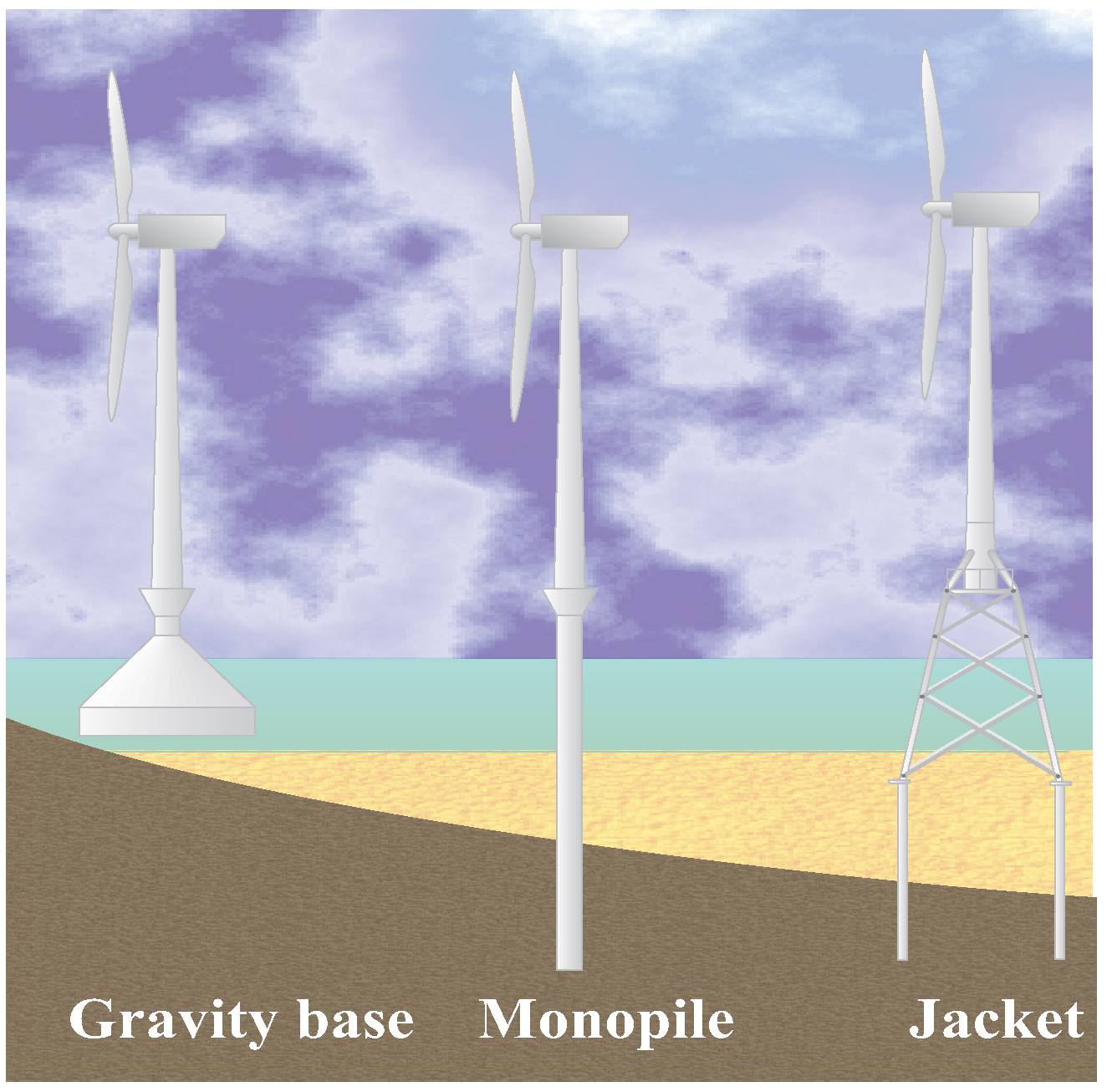
There are more than 7000 offshore structures around the world. Structures to support wind turbines come in various shapes and sizes; the most common are monopile, jacket, tripod, gravity base and floating structures (Figure 1). There are several kinds of platforms, but a fixed structure in a jacket structure is considered in the present paper. The tendency of large-sized offshore wind turbines has increased during the last 10 years. As wind turbines get larger and are located in deeper water, jacket structures are expected to become more attractive. Generally, a fixed platform is described as consisting two main components; the substructure and the superstructure. Superstructure or “topside” is supported on a deck, which is mounted on the jacket structure. The substructure is either a steel tubular jacket or a prestressed concrete structure.
Support structures for offshore wind turbines are highly dynamic, having to cope with combined wind and hydrodynamic loading and complex dynamic behavior from the wind turbine. The offshore jacket platform is a complex and nonlinear system, which can be excited with harmful vibration by the external loads. It is vital to capture the integrated effect of the total loads. However, the total loading can be significantly less than the sum of the constituent loads. This is because the loads are not coincident and because of the existence of different kinds of damping, such as aerodynamic and soil damping, which damps the motions due to the loads. The axial dynamic stiffness of tubular piles is important for offshore wind turbines supported by jacket structures because, in case of overturning moments on the foundation, jacket structures, which are multi-legged structures, mainly rely on vertical capacity. Due to the fixation in the frame, the piles of a jacket (multi-legged) structure deform in an S-shape, mobilizing at the same time horizontal soil resistance. The overturning moment is then transferred as axial loads to opposing foundation piles. The forces are transferred to the seabed by axial forces in the members. The dynamic stiffness indicates the stability and resonance behavior. In fact, the overall weight of modern wind turbines is minimized, which makes them more flexible and, by corollary, more secretive to low frequency dynamics. On the other side, wave propagation in elastic and viscoelastic medium is a considerable issue specially when the medium is earthquakes. In modern offshore wind turbines, the instabilities or stability occur due to the coupled damping of the upper side of the wind turbine and the lower part of that as the foundation. Most of the failure phenomena are caused by fatigue, while the first natural frequency plays an important role. In this aspect, stiffness has a predominant role to evaluate the first natural frequency. The first estimation for the stiffness of the foundation comes through the analysis of soil-structure interaction (SSI). Applying inaccurate algorithms in the soil-structure media may also occur when two different numerical methods are coupled, e.g., the boundary element method (BEM) and the finite element method (FEM); this problem may become even more serious when coupled algorithms and different physical media are considered simultaneously in the same analysis [1]. SSI can be analyzed based on two methods, namely substructure and direct methods, which are highlighted by Wolf [2,3]. Maheshwari and Khatri [4] analyzed an SSI for a combined footing and supporting column on soft soil by using an iterative Gauss elimination technique, while the footing was modeled as a beam having finite flexural rigidity. Soares and Mansur [1] modeled wave propagation in fluid-SSI by using an iterative procedure in BEM based on different kinds of Green functions in order to present the linear and non-linear behavior of elastoplastic regions. Kim et al. [5] studied the two-dimensional wave propagation in a porous seabed by using BEM based on the integral equation, while the numerical results were validated with an analytical solution. Srisupattarawanit et al. [6] applied BEM and a computation method to compute nonlinear random finite depth waves in order to be coupled with an elastic structure. Guenfoud et al. [7] employed Green’s function to solve the integrals resulting from Lamb’s problem in order to study the interaction between soil and structures subjected to a seismic load. Padrón et al. [8] studied the SSI between nearby pile-supported structures in a viscoelastic half-space by using BEM-FEM in the frequency domain. Genes [9] applied a parallelized coupled model based on BEM-FEM to analyze the SSI for arbitrarily-shaped, large-scale SSI problems, and the validation was shown. Comprehensive reviews on applying the methods pertaining to SSI have been done by Mahmoudpour et al. [10] and Wang et al. [11], respectively.
FEM was employed to solve the equations of motion for a two-phase medium by several researchers ([12,13,14,15] and the the references therein). The time domain response of a jacket offshore tower with the soil resistance to the pile movement was modeled using p–y and t–z curves to account for soil nonlinearity and energy dissipation, presented by [16] by employing an finite element (FE) package to do the parameter study. Andersen and Nielsen [17] applied FEM with a transmitting boundary element (BE) and presented a solution in the frequency domain of an elastic half-space to a moving force on its surface. The latter model has been coupled with an FE scheme for the analysis of the shielding efficiency of trenches and barriers along a railway track [18]. Furthermore, a two- and three-dimensional combined FEM and BEM has been carried out for two railway tunnel structures in order to investigate what reliable information can be gained from a two-dimensional model to aid a tunnel design process or an environmental vibration prediction based on “correcting” measured data from another tunnel in similar ground in [19]. Then, the steps in the FEM and BEM formulations were discussed, as well as the problems with describing material dissipation in the moving frame of reference investigated by [20]. Andersen et al. [21] used a numerical method to analyze a nonlinear stochastic p–y curve for the calculation of the monopile response. The time-domain results for soil–foundation–structure interaction by considering the dependence of the foundation on the frequency of excitation were presented by Cazzani and Ruge [22] by using FEM. Furthermore, due to the unbounded nature of a soil medium, the computational size of these methods is very large. For this reason, it is important to establish some simple mathematical models that reduce the computational cost of analysis, as well as increase the accuracy of the results. The FEM requires the discretization of the domain, which has to be simulated as infinite in most SSI problems. This implies a high number of elements, leading to a large and sometimes impracticable processing time. This becomes more viable solving these problems with the BEM, once only the boundary of the domains involved is discretized. This allows reducing the problem dimension, implying less processing time. This advantage is explored in several works [23,24] (see the references therein).
BEM provides a powerful numerical tool for the calculation of dynamic structure response in the frequency and time domain. By implementing the boundary integral method, equations of motion and also boundary conditions are discretized only on the boundary. As we know, soil can be modeled as a semi-infinite domain in SSI analysis. The energy radiation into a surrounding medium is modeled correctly, which is very applicable for infinite and semi-infinite domains. By using this method, the problem dimension is reduced by one and by fulfilling the radiation condition, which represents its advantage for unbounded domains. By employing BEM on the stress-strain relation is a differential or integration method [25]. BEM has the advantages of simplicity to model far field, as the radiation conditions can be satisfied in the analytical fundamental solutions [26]. Betti’s reciprocal theorem has the advantage of linking the solution of two different problems for the same domain of an elastic body. Once the required Green’s functions are obtained, the BEM is formulated with the help of the numerical interpretation of Somigliana’s identity [27]. SSI problems can be investigated in a time domain or a frequency domain. Since the effect of wave propagation in infinite soil is well represented through the frequency-dependent dynamic stiffness of the sub-grade, the frequency domain is advantageous [28].
It may be noted that existing literature on offshore monopile foundations as cited above has been solved experimentally or theoretically based on numerical and analytical methods. To the best of our knowledge, no work has been reported to date that analyzes the jacket foundation as a long hollow cylinder by using an appropriate mathematical approach and employing Green’s function and the integral method. This study attempts to concentrate on this investigation. In this paper, an offshore jacket foundation in an elastic and viscoelastic media is investigated by modeling that as a long tubular pile. The integral method, along with the Betti reciprocal theorem, Somigliana identity and Green’s function, is employed. The vertical loads with low and high frequency are applied on the smooth surface along the entire interface. The effect of material properties, such as Young’s modulus and Poisson’s ratio, on the dynamic stiffness and phase angle are illuminated. This work aims to investigate the effect of some basic factors, such as geometry, damping and frequency, on stiffness, phase velocity and mode of resonance and anti-resonance in the monopile foundation. The singularity of Bessel’s function is investigated. The exact solutions are obtained in the elastic and frequency domain. The modes of resonance and anti-resonance are presented in a series of Bessel functions.
2. General Definition of the Model
Consider a thin axisymmetric smooth long cylinder with constant thickness and mean radius R as shown in Figure 2. This cylinder is subject to harmonically-varying forced displacement with cyclic frequency and applied in the -direction, along the center axis. In this case, the pure antiplane, shear wave propagation (shear/secondary horizontal (SH)-waves) is utilized, which means that there is no displacement in the - or -direction. Axial symmetry in geometry and loading is assumed, and cylindrical coordinates are considered.
The geometry of an infinite cylinder and the definition of polar coordinates: -plane and -plane. An observation point with the plane coordinates is considered, and the material is present on both sides of the cylindrical interface, where the boundaries and are related to domains in Equations (1) and (2), respectively.
3. Theoretical Formulation and Equilibrium Equations
Somigliana’s identity is the simplest theory based on the dynamic reciprocity theorem and the fundamental solution that is used for wave propagation in elastic media. The three-dimensional frequency-domain of Somigliana’s identity reads:
where:
where is a coefficient dependent on the position . In particular, for any interior point within the domain Ω, the constant takes the value . Actually, the value of simply corresponds to the part of the point that is included in the domain Ω. Hence, at an exterior point and for a point on a smooth part of the boundary Γ. Further, at the apex of a cone or pyramid with the internal solid angle , the geometry constant is , and at a wedge point with the internal angle Φ, . A mathematically-sound proof regarding the values of for different geometries of the surface is beyond the scope of the present paper. A detailed derivation for a smooth part of a surface can be found in the work by Dominguez [27]. Finally, in the general case, finding may be difficult, especially at the intersection of multiple curved surfaces.
By assuming that the displacement field, surface traction and body force in the physical state vary harmonically with the circular frequency , then:
where are the components of the displacement field, the surface traction and is the load per unit mass in coordinate direction i. Vector is the position in space, and t is the time. Furthermore, based on the Cauchylaw (), the relation between surface traction and the Cauchy stress tensor is: .
and are the Green’s functions for the displacements and the surface traction in the frequency domain or, in other words, they are the Fourier transforms of and , respectively. It can be mentioned here that Green’s function for a vector field is a second-order tensor with the components , which provides the response at point and time t in coordinate direction i due to a unit magnitude concentrated force acting at the point and time in coordinate direction l. Hence, whereas the displacement field is a vector field with the components , the corresponding Green’s function is a tensor field with the doubly-indexed components .
3.1. Frequency-Domain Equation of the Motion of the Shear/Secondary Horizontal-Wave
The antiplane shear assumption induces the displacement components and , which are identically equal to zero, and partial derivatives with respect to vanish; only the displacement component in the direction out of the -plane exists, and it is constant along the -direction. In the case of elastodynamics, this corresponds to the propagation of SH-waves in the -plane. When antiplane shear is considered, only the third component of the displacement field is different from zero. This holds for both the physical field and Green’s function. Hence, Somigliana’s identity simplifies to a scalar integral equation as:
Further, since the surface is smooth along the entire interface, Somigliana’s identity in Equation (4) for the two domains is reduced to:
where and are the displacements in the -direction along the boundaries and , respectively, whereas and are the corresponding surface traction. In the derivation of Equations (5) and (6), it has been utilized that the surface of the circular cylinder is smooth. The value for points inside domain and for points on the pile surface is ; more details are presented by Dominguez [27]. In order to investigate the continuity conditions in the common boundary between domains and , we are interested in calculations regarding the pile surface. Meanwhile, several shortcomings can be highlighted by considering the infinite length of the pile, such as: dynamic stiffness for an infinite cylinder is greater than that for a finite cylinder (this is illustrated in Figure 3); the results cover vertical response, while for finite piles transverse and axial responses are included; and finally, for a finite length, some responses are related to P-waves and shear/secondary vertical (SV)-waves in addition to SH-waves.
3.2. Green’s Function
The fundamental solutions for the antiplane displacements are (the details and procedure to obtain the fundamental solution are presented in Appendix A):
where is the shear modulus, represents the modified Bessel function of the second kind and order m and is the wavenumber. the relation between wavenumber and phase speed is:
where is dependent on the material properties of the porous media, and it is defined as:
where is the loss factor, and is the material density. For a homogeneous isotropic linear elastic material, the generalized Hooke’s law forming the relation between stresses, , and strains, , simplifies to:
where and are the Lame constants, is the Kronecker delta and is the dilation. Substituting the fundamental displacements () from Equation (7) into Hook’s law (Equation (10)) and applying the Cauchy stress law, the fundamental surface shear stresses are obtained:
where defines the partial derivative of the distance ϱ between the source and observation points, and , in the direction of the outward normal:
Here, is the angle between the distance vector and the normal vector .
3.3. Continuity Conditions
The continuity conditions at the interfaces of the displacements across the interface for the forced displacement with constant amplitude and in phase along the cylindrical interface, , provide the result:
3.4. Analysis
According to the frequency-domain equation of motion for each domain, inside and outside of the cylinder, the dynamic stiffness can be obtained. Eliminating from Equations (14) and (15), the constant amplitude can be written in terms of the traction on the interface, as follows:
where the mean traction on either side of the interface () is:
The general dynamic stiffness () per unit surface of the interface related to displacement along the cylinder axis for arbitrary geometry of the infinite cylinder becomes:
where is the length of the interface Γ, measured in the -plane. In the presented case, an offshore foundation is considered as an infinite circular cylinder with radius R that is with . In order to compute , the cylindrical polar coordinates are introduced (Figure 2), such that:
In these coordinates, the boundary Γ is defined by , , .
In particular, when an observation point with the plane coordinates is considered (Figure 2), the distance ϱ between the source and observation point becomes:
Making use of the fact that , Equation (16) may then be evaluated as:
Here, is the Bessel function of the first kind and order zero. It is noted that for . Hence, for . Furthermore, has a number of zeros for and . At the corresponding frequencies, becomes singular.
3.5. Reference Solution by Coupled Boundary Element Method/Finite Element Method
By considering Somigliana’s identity presented in Equation (1) and assuming that no forces are applied in the interior of the domain, Somigliana’s identity is evaluated by the discrimination of the displacement () and traction () fields into the nodal values and interpolation by local shape functions at the nodes of BE j over space as:
On the other side, the FEM, the equation of motions can be written as:
where , and are the mass, hysteretic damping and stiffness matrices, respectively, while the hysteretic material damping is . and are the nodal displacements and forces, respectively, which represent the coupling between FE and BE regions. This entails that each BE domain can be transformed into macro FE, as shown in Figure 4. Here, in Figure 4 is a transform matrix, which is frequency independent, expressing the relationship between the nodal forces in the FE domain and surface traction in the BE domain. Quadratic shape functions by using Green’s functions as weight functions and as shape functions in a standard Galerkin FEM scheme were employed by Andersen and Jones [29]. More information is in [29]. The three-dimensional coupled BE/FE has been implemented in the computer code BEASTS [30].
For the verification of the results of the present study, the results from the BEASTS program created by Andersen and Jones [29] to estimate the dynamic stiffness of a simple model of an offshore wind turbine with different lengths were considered. A graph of the dynamic stiffness against non-dimensional frequency is given in Figure 5 having the material properties as: , density = 2000 , Poisson’s ratio , loss factor and also R = 3.0 m. As shown in Figure 5, the results for the dimensionless stiffness of this study are very well comparable with those of Andersen et al. [31]. As expected, by increasing the length of the pile in BEASTS, the results converge to those in a pile with infinite length. The radius is considered three (m), and then, different lengths of pile are considered, which are multiples of the radius, the main reason being to have a large value of length with respect to radius. The same pattern can be seen in Figure 5 and the presented results in [31]. It can be noted that the same kind of phenomenon is investigated (in Figure 5 and [31]); only one type of wave is involved. The results in Figure 5 show more or less the same overall trend; the stiffness is going to increase and then decrease, and this pattern is going to repeat by varying the normalized frequency (the same as Figure 5 in [31]). The results quantify the finite pile with the infinite pile.
4. Numerical Results
For numerical illustration of the elastic solutions of this study, a thin long hollow cylinder with mean radius R = 3.0 m is considered. Young’s modulus is considered between and , while the density is = 1861 , the same as considered in [32]. The interval of the loss factor () related to the damping is 0.01–0.1 [33].
4.1. Results and Discussion
In the following, results are presented in non-dimensional frequency and the normalized dynamic stiffness , where the impedance by considering different values of material properties, such as Young’s modulus, loss factor, resonance and anti-resonance frequencies.
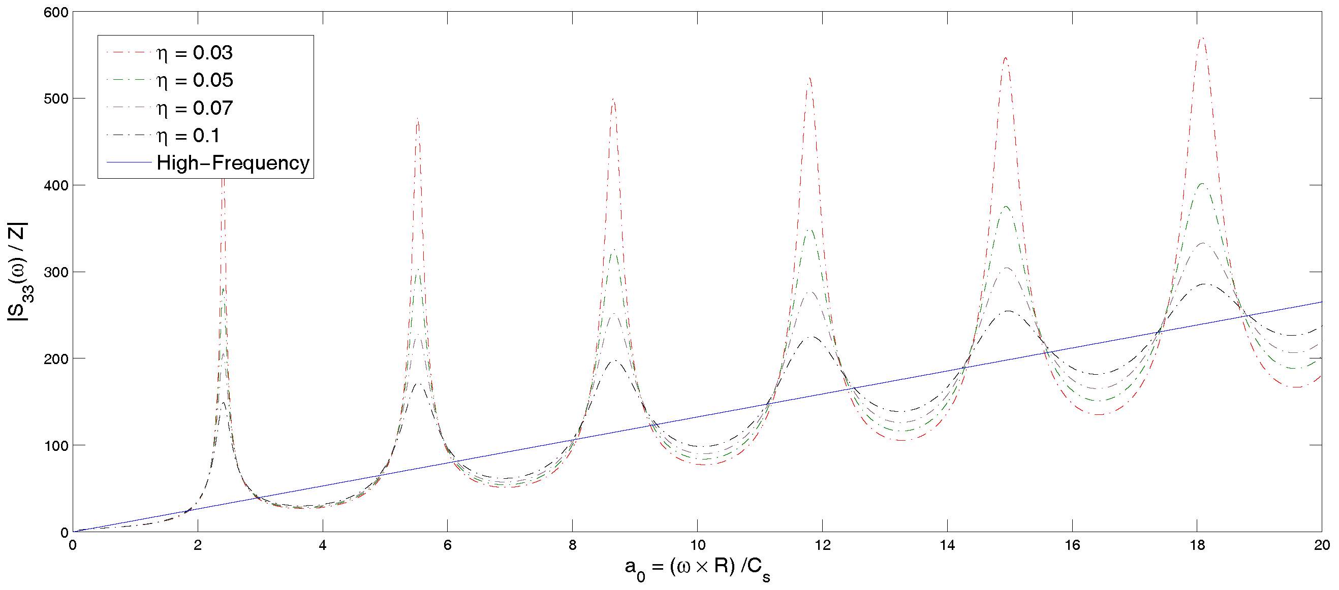
Figure 6 illustrates the non-dimensional dynamic stiffness based on the small deformation theory due to axial force. This figure contains graphs for different values of the loss factor in Equation (8) using . The value of stiffness increases with the increase of the load frequency until reaching a peak point, then decreases to a local minimum for a certain value of frequency and, again, increases with the increase of the load frequency to the next peak point. This procedure is repeated in an oscillatory manner. The local peak point for dynamic stiffness decreases with increasing loss factor, whilst the local minimum point of the stiffness increases with decreasing the loss factor. It can be noticed that the turning point, at which the concave curve changes into the convex curve, is the same for all different loss factors.
Figure 7 shows the effect of Young’s modulus E on the variation of the dynamic stiffness vs. load frequency. The non-dimensional dynamic stiffness has a greater value with respect to soil with a lower Young’s modulus for all values of load frequency. It is worth mentioning that the difference between dynamic stiffness for a higher value of load frequency is greater than those for lower load frequency. As expected, these results confirm that soil with a greater Young’s modulus has greater dynamic stiffness, and this conclusion is the same as in earlier results reported by [27,33] and the presented results from Andersen and Jones [30], as shown in Figure 5.
The variation of the dynamic stiffness with load frequency is shown in Figure 8 for different values of Poisson’s ratio. It is observed that the smaller Poisson’s ratio introduces greater dynamic stiffness. The difference between stiffness is increasing when the load frequency is increased, which is the same observation in Figure 7, which is related to different values of the shear modulus.
The results of Figure 7 and Figure 8 can be summarized to conclude that the dynamic stiffness in an infinite cylinder with a greater shear modulus and a smaller Poisson’s ratio is larger than those with a smaller shear modulus and a greater Poisson’s ratio. A similar result has been reported in [27,30,33], respectively.
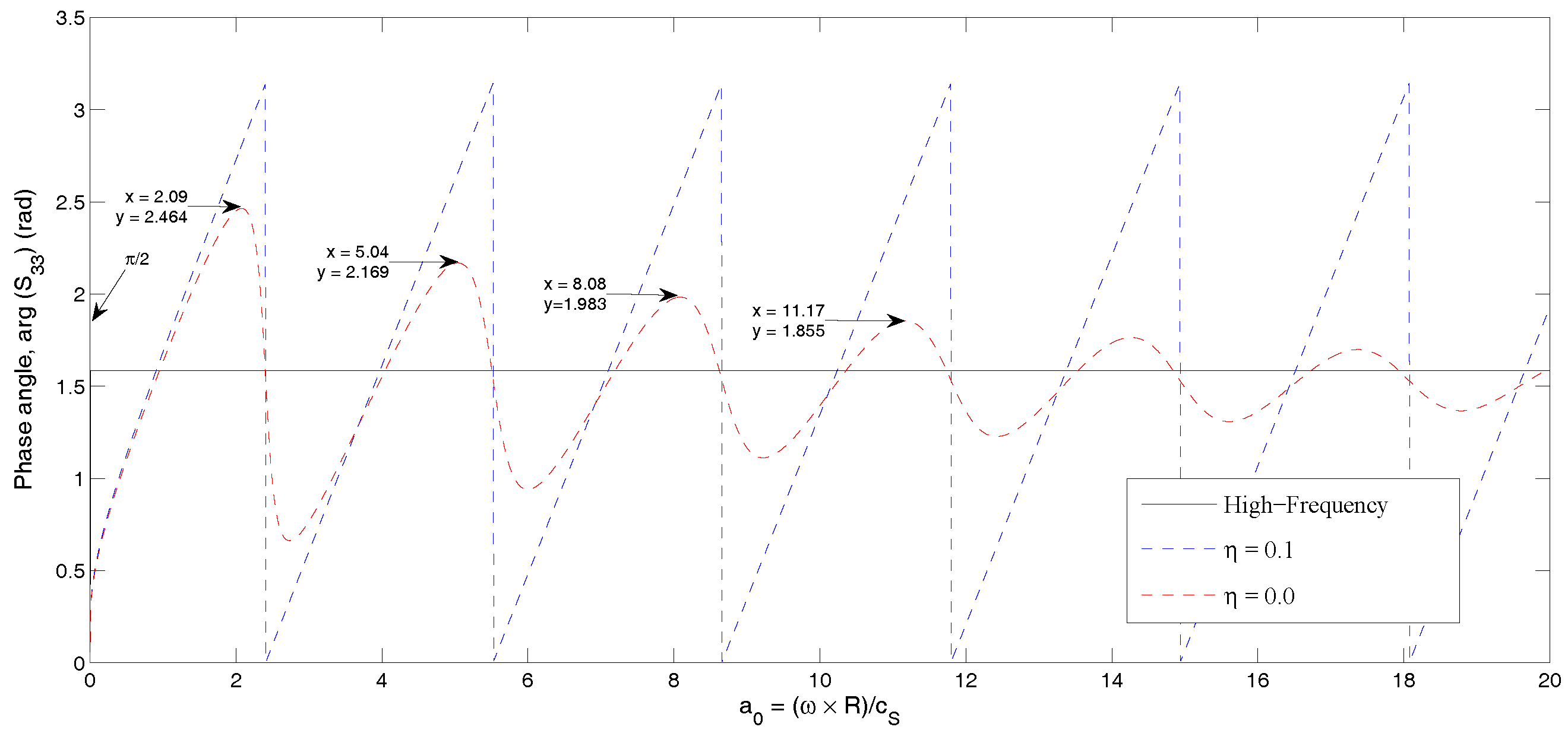
Figure 9 in the following compares the phase angle for dynamic stiffness vs. non-dimensional load frequency with different values of the loss factor. As seen, the phase angle oscillating around line and the amount of fluctuation around this line decreases with the increase of load frequency. It can be noted that the absolute value of the maximum or minimum value of the phase angle and central line (line ) decreases with the increase of load frequency.
Figure 10 and Figure 11 concern the comparison of the phase angle for dynamic stiffness versus non-dimensional load frequency for different values of Young’s modulus and Poisson’s ratio. In contrast with the results for different values of the loss factor, other material properties, such as Young’s modulus and Poisson’s ratio, do not have any effect on the phase angle, like the results reported in [27,33].
4.2. High Frequency Results
In the high frequency limit, the complex stiffness becomes a pure impedance [27]. Based on the similarity of direct electrical and alternating current principles and borrowing the concept of ohmic resistance from Ohm’s law to present the electrical impedance, the acoustic impedance (z) is defined as the ratio between the pressure, p, and the particle velocity, v, on an imaginary surface in a sound wave, . An acoustic impedance is , where is the mass density of the material and c is a characteristic phase velocity of the wave propagation in the material. Thus, in contrast to the electrical impedance, which is a complex quantity in the frequency domain, the acoustic impedance is real valued. The impedance at a point on the inside or the outside of the cylinder is . Integrating over the area of the cylinder, including the interior, as well as the exterior surface, the impedance of the cylinder per unit length in the axial direction becomes . R is the radii of the pile.
The dynamic stiffness in the high frequency limit is derived from the definition of the impedance. In the time domain, the surface traction is related to the particle velocity as , where the superscript ∞ indicates that the limit . Accordingly, in the frequency domain, the relationship becomes . Hence, including the contributions from both sides of the cylinder, , as well as , the dynamic stiffness may be written as:
The dynamic stiffness due to high frequency load versus non-dimensional load frequency is shown in Figure 12. As seen in the figure, the non-dimensional dynamic stiffness changes linearly with the load frequency as expected from Equation (25). The other results for different values of the loss factor in low frequency have been shown in order to compare the results for high frequency and low frequency loads. In Figure 12, the dynamic stiffness approaches the high frequency solution for and increasing values of the loss factor. Hence, when , the dynamic stiffness is almost identical to , even at relatively low values of the non-dimensional frequency .
It is evident from Figure 13 that the phase angle of dynamic stiffness for high-frequency load is constant and equal to , as expected from Equation (25). It is noted that the phase angle of the dynamic stiffness is always negative. Hence, has been plotted in the figure.
Further, it is known that the solution for is singular at a number of frequencies within the considered frequency interval. Actually, these singularities occur at the roots of .
4.3. Mode of Resonance and Anti-Resonance
To present the mode of resonance and anti-resonance, the load frequency related to the minimum and maximum value dynamic stiffness is needed. In order to calculate the related frequency, the maximum non-dimensional frequency shown in Figure 14, which is related to Section A in Figure 14, is needed. Furthermore, the frequency related to Section B in Figure 14 is needed.
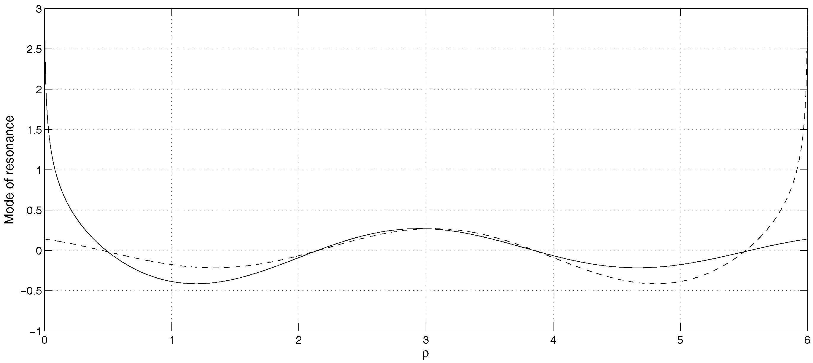
Figure 15 presents the schematic wave mode inside the cylinder versus ϱ (, from Equation (20)). The value of non-dimensional frequency is taken from Section A in Figure 14, and here, is employed to highlight the mode shape of two points on the pile surface with the biggest distance. Actually, by selecting each value of to correspond with the peak point (such as = 2.42, (or =) 5.53, (or =) 8.67, (or =) 11.83), the resonance mode can be seen. As was mentioned, the presented mode for two points has a distance equal to the pile diameter. For these two points and the mentioned frequency, the resonance mode is observed. The continuous line represents the wave motion from the left-hand side of the cylinder toward the right-hand side, and the dashed line represents the wave motion from the right- to left-hand side of cylinder. As seen, the wave motion on the left-hand side or right-hand side has the same sign; in the figure, both of them are positive, which means the resonance phenomena.
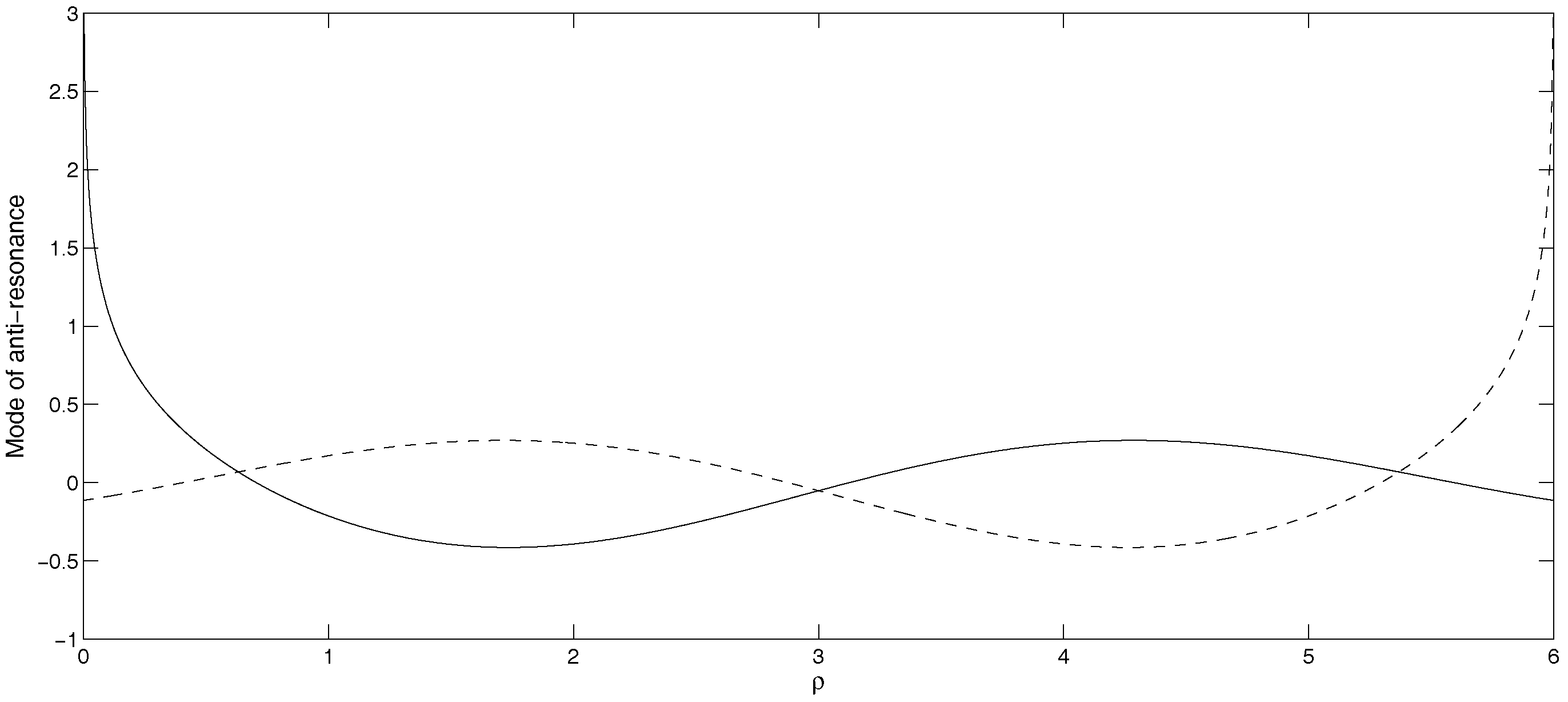
Figure 16 presents the schematic anti-resonance mode inside the cylinder versus ϱ. The value of non-dimensional frequency is taken from Figure 14, which belongs to Section B in Figure 14, and here, . As seen, the wave motion on the left-hand side or right-hand side does not have the same sign. In the figure, one of them is positive, and the other is negative, which means the anti-resonance phenomena. It should be mentioned that for the mentioned frequency, while the distance of the two points is equal to the pile diameter, the anti-resonance is observed. However, for the same frequency and employing the other two points, the resonance and anti-resonance can be observed. As can be seen from the continuous (or dashed) line, most points on the continuous (or dashed) line are positive, which is conducted to have the maximum stiffness with the employed frequency.
5. Conclusions
Offshore jacket wind turbine foundations are modeled as smooth long cylinders, while being subjected to dynamic vertical excitation. A mathematical approach, like the boundary integral method, is employed to find the exact dynamic stiffness of the jacket foundation, phase angle, resonance and anti-resonance mode. The jacket foundation is considered in a viscoelastic media, and elastic responses are presented by using the Betti reciprocal theorem, Somigliana’s identity and Green’s function. The behavior of the soil with damping and without damping is explored. Furthermore, the effects of material properties, such as Young’s modulus and Poisson’s ratio, are investigated. The results for the soil with the loss factor are validated and compared. Some general observations of this study can be summarized as:
- The dynamic stiffness increases with the increase of the load frequency until reaching a peak point, then decreases to a local minimum for a certain value of frequency and, again, increases with the increase of the load frequency to the next peak point. This procedure is repeated in an oscillatory manner.
- The local peak point for dynamic stiffness decreases with the increasing loss factor, whilst the local minimum point of the stiffness increases with decreasing the loss factor. It is worth mentioning that the turning point at which the concave curve changes into convex curve is the same for all different loss factors. Furthermore, the turning point increases with the increase of the load frequency whilst it is independent of the loss factor for a certain value of load frequency.
- The phase angle for dynamic stiffness is changing with the variation of the loss factor, whilst it is constant for different values of Young’s modulus and Poisson’s ratio.
It is observed using a mathematical approach that pertains to the vertical vibration analysis that this provides a good understanding about the behavior of soil, besides the wave propagation and different modes of the wave. The results reveal that the presented approach gains the physical understanding for offshore foundations in the geomechanics field.
Acknowledgments
Authors highly appreciate the financial support provided by the Danish Energy Development and Demonstration Programme (EUDP) (Grant No. is 64010-0124, EUDP 10-I and Project No. in Aalborg University is 826059) via the Project “Monopile Cost Reduction and Demonstration by Joint Applied Research”, and also from The Danish National Advanced Technology Foundation (HTF) Funded Project via the Project “Cost Effective Mass Production of Universal Foundation for Large Offshore Wind Parks”, (Universal Foundation, FORCE Technology, LIC Engineering, DTU Wind Energy, Technology Foundation and Aalborg University (AAU)).
Author Contributions
This paper is a result of the collaboration of all co-authors. Mehdi Bayat and Lars Vabbersgaard Andersen established the model and programming. Lars Bo Ibsen proposed and highlighted the effect of different soil types. Mehdi Bayat was mainly responsible for the numerical simulation, results’ interpretation and initial writing. All co-authors performed editing and reviewing of the paper.
Conflicts of Interest
The authors declare no conflict of interest.
Appendix A: Fundamental Solution
Wave propagation in the full space is governed by the Navier equations. Inserting the specific body forces into the Navier equations, the time-domain Green’s function for scalar wave propagation in a homogeneous isotropic full space is defined by the equation:
In order to solve the above equation, by assuming that the load is applied at the origin, , and applying the Laplace operator, the symmetry condition, the divergence theorem, physical reasons and Fourier transformation on the obtained time-domain solution, the frequency-domain fundamental solution reads:
where is the Hankel function of the second kind and order zero, whereas is the modified Bessel function of order zero. It is noted that . More details and further information can be found in [27].
References
- Soares, D., Jr.; Mansur, W. Dynamic analysis of fluid-soil-structure interaction problems by the boundary element method. J. Comput. Phys. 2006, 219, 498–512. [Google Scholar] [CrossRef]
- Wolf, J.P. Dynamic Soil-Structure Interaction; Prentice-Hall: Englewood Cliffs, NJ, USA, 1985. [Google Scholar]
- Wolf, J.P. Soil Structure Interaction Analysis in Time Domain; Prentice-Hall: Englewood Cliffs, NJ, USA, 1988. [Google Scholar]
- Maheshwari, P.; Khatri, S. A nonlinear model for footings on granular bed-stone column reinforced earth beds. Appl. Math. Model. 2011, 35, 2790–2804. [Google Scholar] [CrossRef]
- Kim, M.; Koo, W.; Hong, S.Y. Wave interactions with 2D structures on/inside porous seabed by a two-domain boundary element method. Appl. Math. Model. 2000, 22, 255–266. [Google Scholar] [CrossRef]
- Srisupattarawanit, T.; Niekamp, R.; Matthies, H. Imulation of nonlinear random finite depth waves coupled with an elastic structure. Comput. Methods Appl. Mech. Eng. 2006, 195, 3072–3086. [Google Scholar] [CrossRef]
- Guenfouda, S.; Amrane, M.; Bosakov, V.; Ouelaa, N. Semi-analytical evaluation of integral forms associated with Lamb’s problem. Soil Dyn. Earthq. Eng. 2009, 29, 438–443. [Google Scholar] [CrossRef]
- Padrón, L.A.; Aznárez, J.J.; Maeso, O. Dynamic structure-soil-structure interaction between nearby piled buildings under seismic excitation by BEM-FEM model. Soil Dyn. Earthq. Eng. 2009, 29, 1084–1096. [Google Scholar] [CrossRef]
- Genes, M.C. Dynamic analysis of large-scale SSI systems for layered unbounded media via a parallelized coupled finite-element/boundary-element/scaled boundary finite-element model. Eng. Anal. Bound. Elem. 2012, 36, 845–857. [Google Scholar] [CrossRef]
- Mahmoudpour, S.; Attarnejad, R.; Behnia, C. Dynamic analysis of partially embedded structures considering soil-structure interaction in time domain. Math. Probl. Eng. 2011, 2011. [Google Scholar] [CrossRef]
- Wang, H.-F.; Lou, M.-L.; Xi, C.; Zhai, Y.-M. An overview of structure-soil-structure dynamic interaction research. J. Chongqing Univ. 2011, 10, 101–112. [Google Scholar]
- Zienkiewicz, O.C. Basic formulation of static and dynamic behaviours of soil and other porous media. Appl. Math. Mech. 1982, 3, 457–468. [Google Scholar] [CrossRef]
- Prevost, J.H. Nonlinear transient phenomena in saturated porous media. Comput. Methods Appl. Mech. Eng. 1982, 20, 3–18. [Google Scholar] [CrossRef]
- Jeremi, B.; Cheng, Z.; Taiebat, M.; Dafalias, Y. Numerical simulation of fully saturated porous materials. Int. J. Numer. Anal. Methods Geomech. 2008, 32, 1635–1660. [Google Scholar] [CrossRef]
- Bayat, M.; Ghorashi, S.S.; Amani, J.; Andersen, L.V.; Ibsen, L.B.; Rabczuk, T.; Zhuang, X.; Talebi, H. Recovery-based error estimation in the dynamic analysis of offshore wind turbine monopile foundations. Comput. Geotech. 2015, 70, 24–40. [Google Scholar] [CrossRef]
- Mostafa, Y.E.; Naggar, M.E. Response of fixed offshore platforms to wave and current loading including soil-structure interaction. Soil Dyn. Earthq. Eng. 2004, 24, 357–368. [Google Scholar] [CrossRef]
- Andersen, L.; Nielsen, S.R.K. Boundary element analysis of the steadystate response of an elastic half-space to a moving force on its surface. Eng. Anal. Bound. Elem. 2003, 27, 23–38. [Google Scholar] [CrossRef]
- Andersen, L.; Nielsen, S.R.K. Coupled Finite Element/Boundary Element Analysis of a Vehicle Moving along a Railway Track. In Proceedings of the 11th International Conference on Soil Dynamics and Earthquake Engineering, Berkeley, CA, USA, 7–9 January 2004; Doolin, D., Kammerer, A., Nogami, T., Seed, R.B., Towhata, I., Eds.; University of California, Berkeley: Berkeley, CA, USA, 2004; pp. 869–876. [Google Scholar]
- Andersen, L.; Jones, C.J.C. Coupled boundary and finite element analysis of vibration from railway tunnels—A comparison of two-and three-dimensional models. J. Sound Vib. 2006, 293, 611–625. [Google Scholar] [CrossRef]
- Andersen, L.; Nielsen, S.R.K.; Krenk, S. Numerical methods for analysis of structure and ground vibration from moving loads. Comput. Struct. 2007, 85, 43–58. [Google Scholar] [CrossRef]
- Andersen, L.; Vahdatirad, M.J.; Sichani, M.T.; Sørensen, J.S. Natural frequencies of wind turbines on monopile foundations in clayey soils—A probabilistic approach. Comput. Geotech. 2012, 43, 1–11. [Google Scholar] [CrossRef]
- Cazzania, A.; Ruge, P. Numerical aspects of coupling strongly frequency-dependent soil-foundation models with structural finite elements in the time-domain. Soil Dyn. Earthq. Eng. 2012, 37, 56–72. [Google Scholar] [CrossRef]
- Ribeiro, D.B.; de Paiva, J.B. Mixed FEM-BEM Formulations Applied to Soil-Structure Interaction problems. In Proceedings of the World Congress on Engineering 2014, London, UK, 2–4 July 2014; pp. 2–4.
- Ai, Z.Y.; Cheng, Y.C. Analysis of vertically loaded piles in multi-layered transversely isotropic soils by BEM. Eng. Anal. Bound. Elem. 2013, 37, 327–335. [Google Scholar] [CrossRef]
- Kompis, V. Selected Topics in Boundary Integral Formulations for Solids and Fluids; Springer-Verlag GmbH: Wien, Austria, 2002. [Google Scholar]
- Zhang, C.; Wolf, J.P. Dynamic Soil-Structure Interaction: Developments in Geotechnical Engineering; Elsevier Science Ltd: Amsterdam, The Netherlands, 1998. [Google Scholar]
- Dominguez, J. Boundary Elements in Dynamics; Computational Mechanics Publications: Southampton, UK, 1993. [Google Scholar]
- Kolekovz, Y.; Schmid, G. Advantages of an analysis of SSI in a frequency domain. Slovak J. Civil Eng. 2011, 4, 12–17. [Google Scholar]
- Andersen, L.; Jones, C. Three-Dimensional Elastodynamic Analysis Using Multiple Boundary Element Domains; University of Southampton: Southampton, UK, 2001. [Google Scholar]
- Andersen, L.; Jones, C. BEASTS—A Computer Program for Boundary Element Analysis of Soil and Three-Dimensional Structures; University of Southampton: Southampton, UK, 2001. [Google Scholar]
- Andersen, L.; Ibsen, L.B.; Liingaard, M.A. Impedance of Bucket Foundations: Torsional, Forizontal and Rocking Motion. In Proceedings of the Sixth International Conference on Engineering Computational Technology, Athens, Greece, 2–5 September 2008; pp. 1–20.
- Barari, A.; Ibsen, L.B. Undrained response of Bucket foundations to moment loading. Appl. Ocean Res. 2012, 36, 12–21. [Google Scholar] [CrossRef]
- Liingaard, M.; Andersen, L.; Ibsen, L. Impedance of flexible suction caissons. Earthq. Eng. Struct. Dyn. 2007, 36, 2249–2271. [Google Scholar] [CrossRef]
Figure 1.
Generic foundation types for offshore wind.

Figure 2.
Geometry of the monopile foundation, Cartesian and polar coordinate systems.
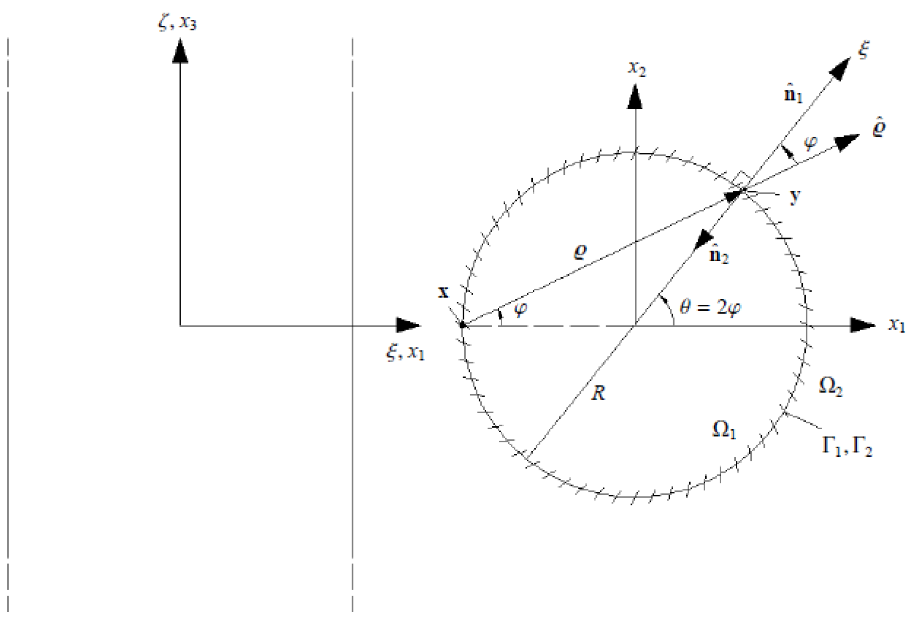
Figure 3.
Geometry of the viscoelastic media, domains and , boundaries and .
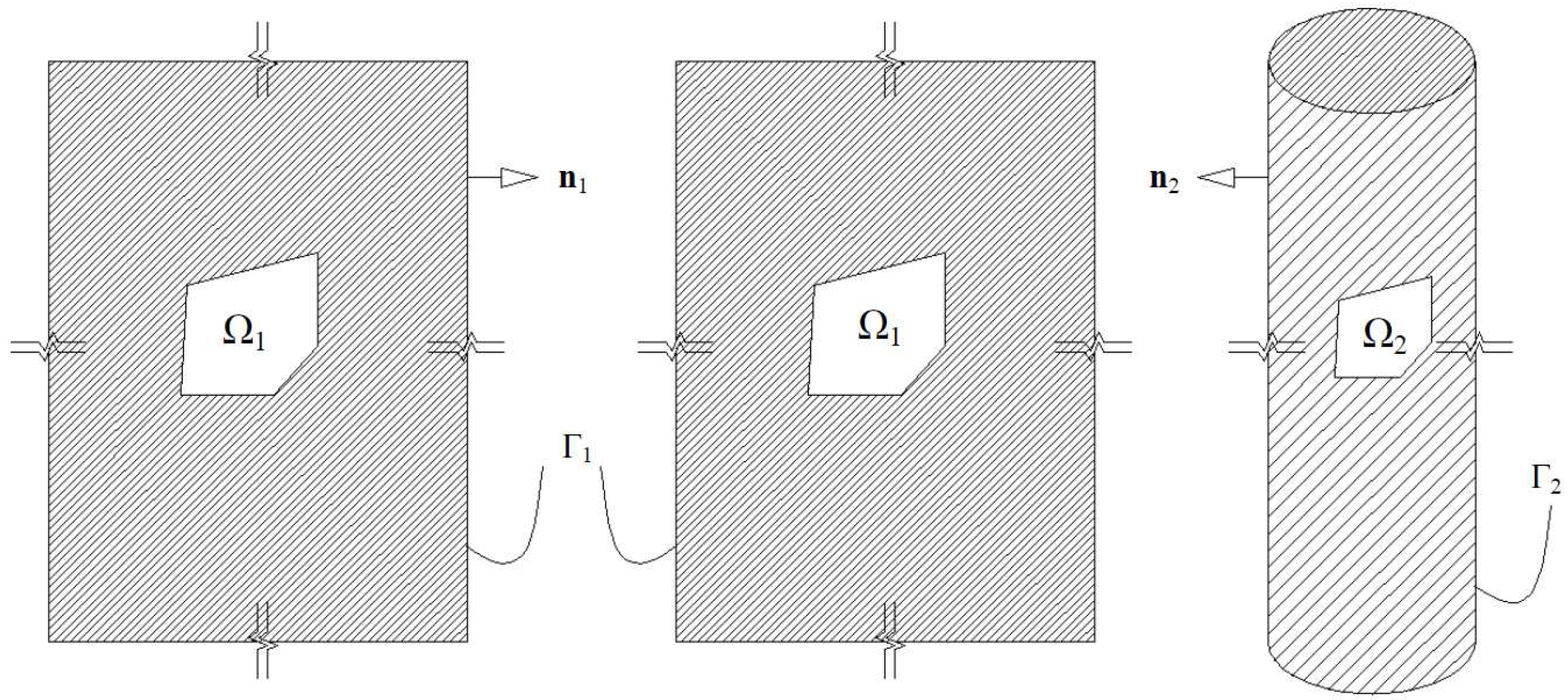
Figure 4.
Coupling of finite element (FE) with a boundary element (BE) domain.
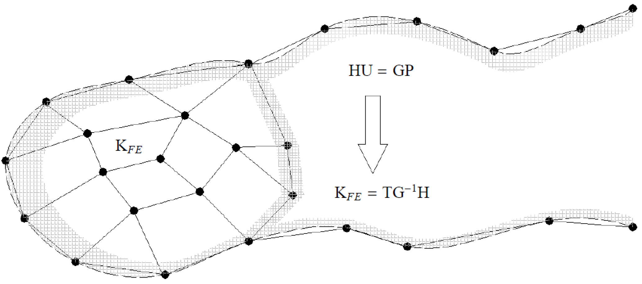
Figure 5.
Comparison between dimensionless stiffness from the presented study and the results from boundary element method (BEM)/finite element method (FEM) in BEASTS by Andersen and Jones [30].
Figure 5.
Comparison between dimensionless stiffness from the presented study and the results from boundary element method (BEM)/finite element method (FEM) in BEASTS by Andersen and Jones [30].
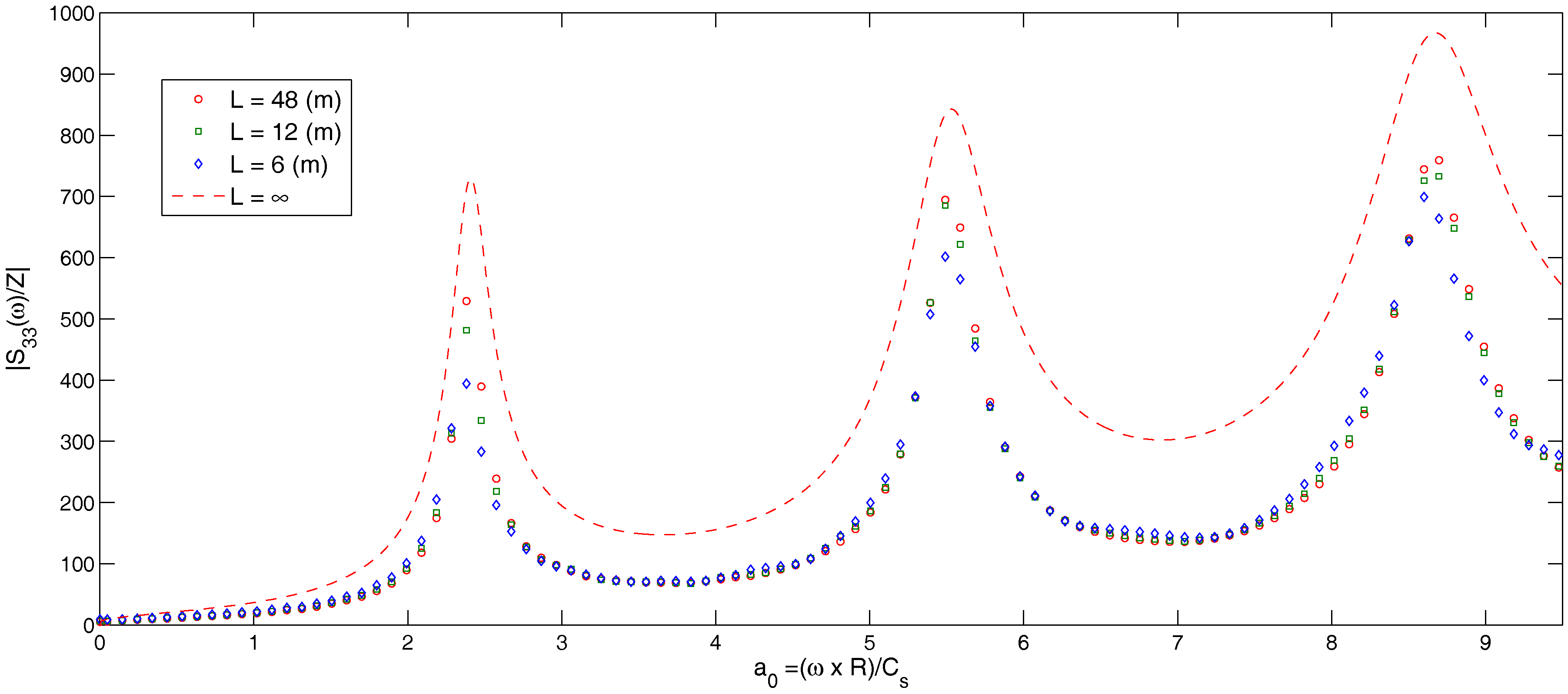
Figure 6.
Non-dimensional dynamic stiffness per unit length of an infinite cylinder due to dynamic vertical load in the axial direction for different values of the loss factor , when and .
Figure 6.
Non-dimensional dynamic stiffness per unit length of an infinite cylinder due to dynamic vertical load in the axial direction for different values of the loss factor , when and .
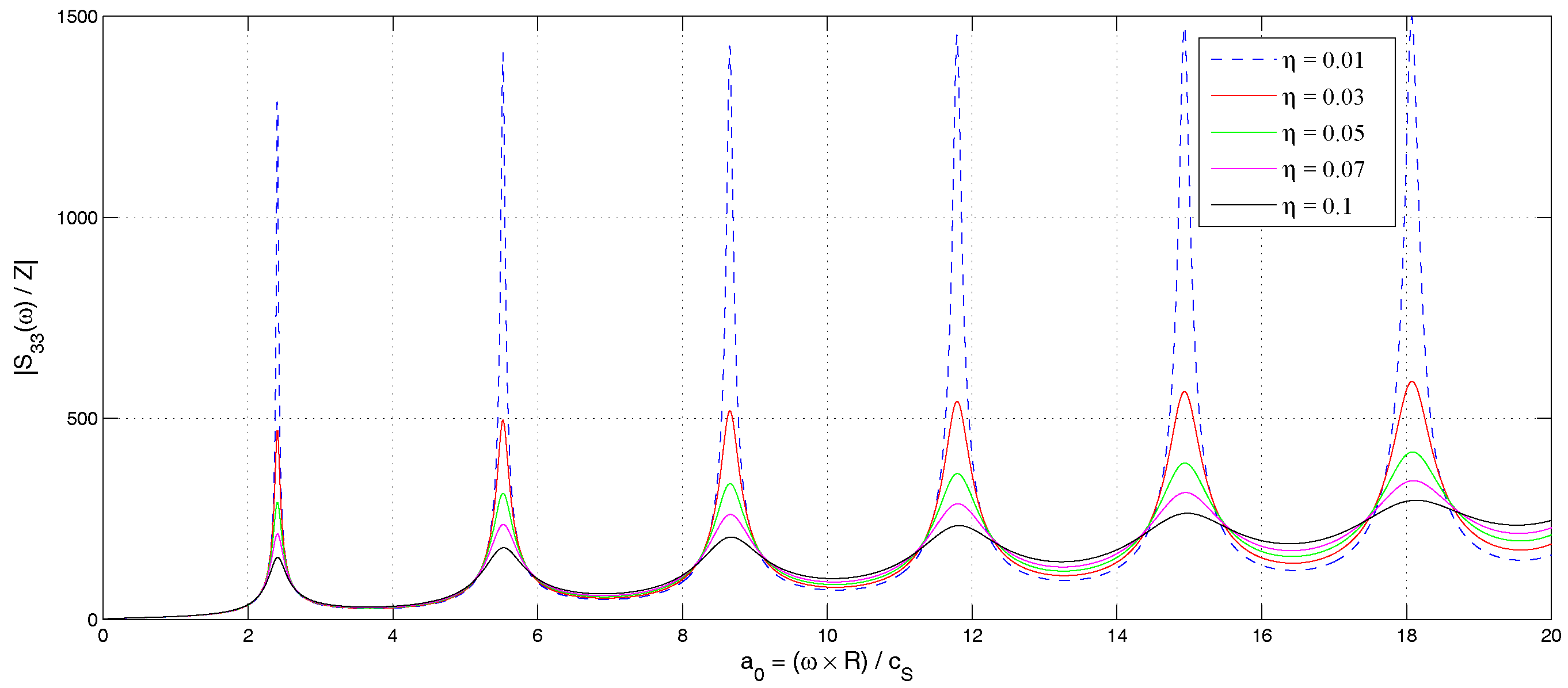
Figure 7.
Non-dimensional dynamic stiffness per unit length of an infinite cylinder due to dynamic vertical load in the axial direction for different values of the Young’s modulus and when loss factor and .
Figure 7.
Non-dimensional dynamic stiffness per unit length of an infinite cylinder due to dynamic vertical load in the axial direction for different values of the Young’s modulus and when loss factor and .
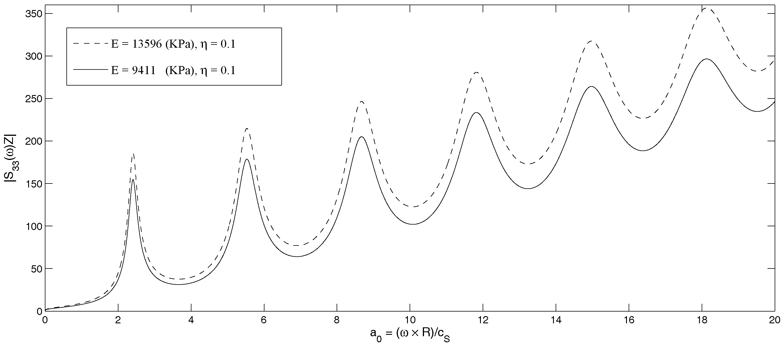
Figure 8.
Non-dimensional dynamic stiffness per unit length of an infinite cylinder due to dynamic vertical load in the axial direction for different values of the Poisson ratio and when the loss factor and .
Figure 8.
Non-dimensional dynamic stiffness per unit length of an infinite cylinder due to dynamic vertical load in the axial direction for different values of the Poisson ratio and when the loss factor and .
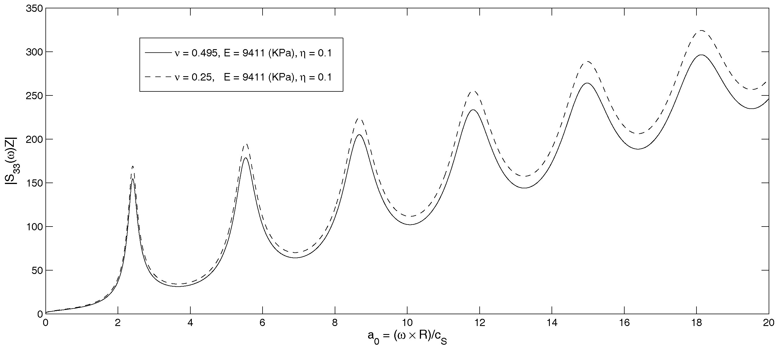
Figure 9.
Phase angle of an infinite cylinder due to dynamic vertical load in the axial direction for different values of the loss factor when loss factor and .
Figure 9.
Phase angle of an infinite cylinder due to dynamic vertical load in the axial direction for different values of the loss factor when loss factor and .
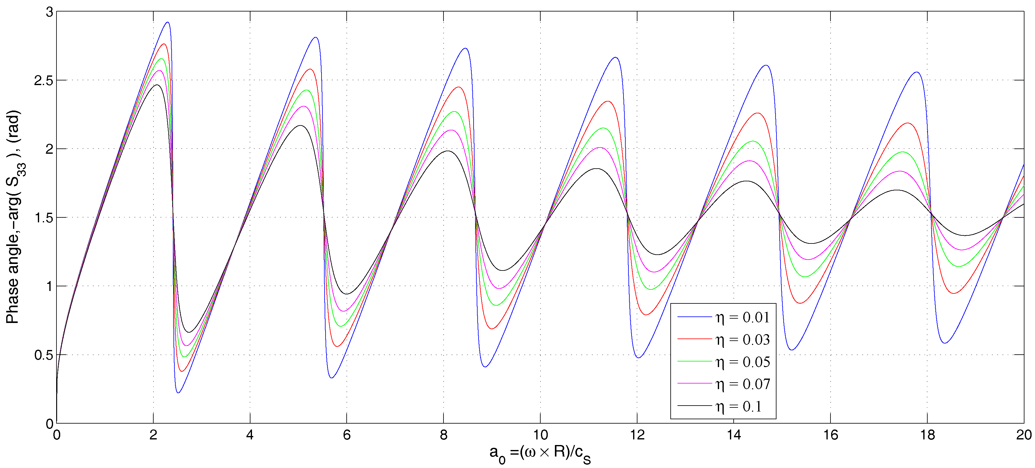
Figure 10.
Phase angle of an infinite cylinder due to dynamic vertical load in the axial direction for different values of Young’s modulus KPa and KPa when the loss factor and .
Figure 10.
Phase angle of an infinite cylinder due to dynamic vertical load in the axial direction for different values of Young’s modulus KPa and KPa when the loss factor and .

Figure 11.
Phase angle of an infinite cylinder due to dynamic vertical load in the axial direction for different values of Poisson’s ratio and when the loss factor and KPa.
Figure 11.
Phase angle of an infinite cylinder due to dynamic vertical load in the axial direction for different values of Poisson’s ratio and when the loss factor and KPa.
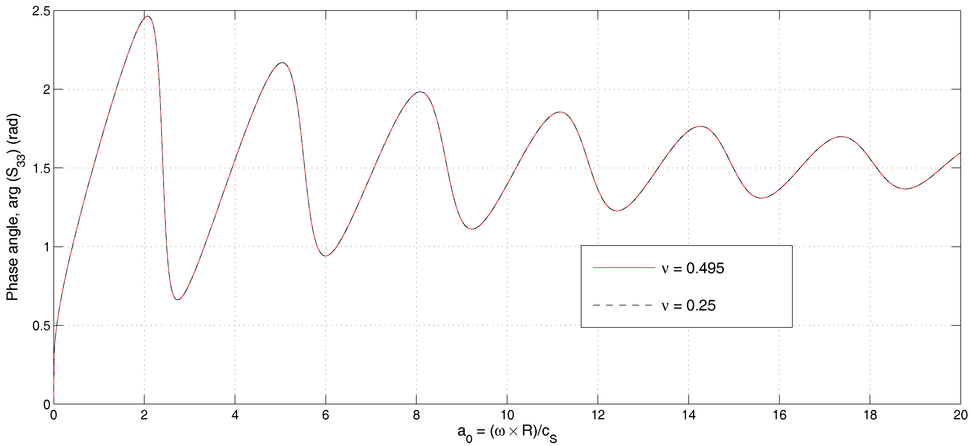
Figure 12.
Dynamic stiffness due to high frequency vertical load in the axial direction (continuous line), which is accompanied by the low frequency results (dash lines) with different values of the loss factor when and KPa.
Figure 12.
Dynamic stiffness due to high frequency vertical load in the axial direction (continuous line), which is accompanied by the low frequency results (dash lines) with different values of the loss factor when and KPa.

Figure 13.
Phase angle of dynamic stiffness due to high frequency vertical load in the axial direction, which is accompanied by the low frequency results with different values of the loss factor when and KPa.
Figure 13.
Phase angle of dynamic stiffness due to high frequency vertical load in the axial direction, which is accompanied by the low frequency results with different values of the loss factor when and KPa.

Figure 14.
Non-dimensional dynamic stiffness due to high and low frequency vertical load in the axial direction for different values of loss factor and when and KPa.
Figure 14.
Non-dimensional dynamic stiffness due to high and low frequency vertical load in the axial direction for different values of loss factor and when and KPa.
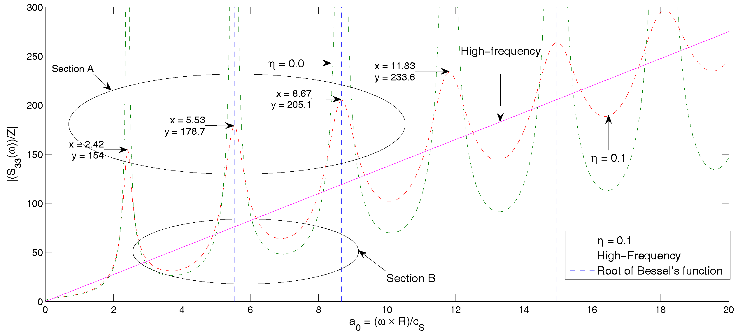
Figure 15.
Scaled mode shape resonance due to load with non-dimensional when the loss factor and KPa.
Figure 15.
Scaled mode shape resonance due to load with non-dimensional when the loss factor and KPa.

Figure 16.
Scaled mode shape resonance due to the load with non-dimensional when the loss factor and KPa.
Figure 16.
Scaled mode shape resonance due to the load with non-dimensional when the loss factor and KPa.
© 2016 by the authors; licensee MDPI, Basel, Switzerland. This article is an open access article distributed under the terms and conditions of the Creative Commons Attribution (CC-BY) license (http://creativecommons.org/licenses/by/4.0/).
Share and Cite
MDPI and ACS Style
Bayat, M.; Andersen, L.V.; Ibsen, L.B. Axial Dynamic Stiffness of Tubular Piles in Viscoelastic Soil. Energies 2016, 9, 734. https://doi.org/10.3390/en9090734
AMA Style
Bayat M, Andersen LV, Ibsen LB. Axial Dynamic Stiffness of Tubular Piles in Viscoelastic Soil. Energies. 2016; 9(9):734. https://doi.org/10.3390/en9090734
Chicago/Turabian StyleBayat, Mehdi, Lars Vabbersgaard Andersen, and Lars Bo Ibsen. 2016. "Axial Dynamic Stiffness of Tubular Piles in Viscoelastic Soil" Energies 9, no. 9: 734. https://doi.org/10.3390/en9090734
Note that from the first issue of 2016, this journal uses article numbers instead of page numbers. See further details here.