
Numerical Simulation on Seismic Response of the Filled Joint under High Amplitude Stress Waves Using Finite-Discrete Element Method (FDEM)

Abstract
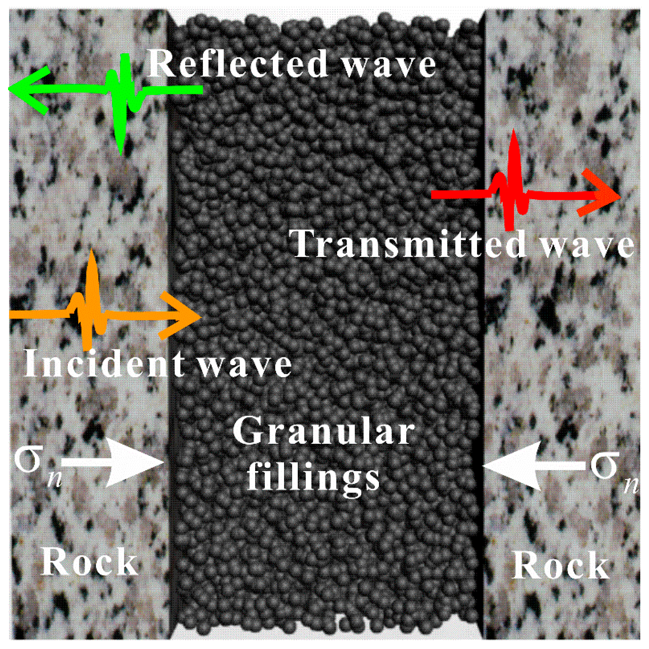
:1. Introduction
2. FDEM Modelling
2.1. Principles of FDEM
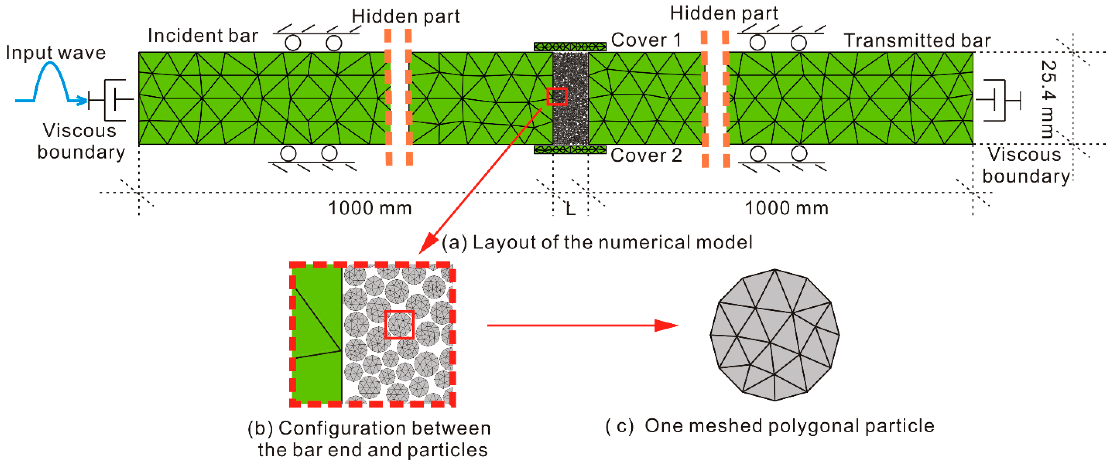
2.2. Model Description
2.3. Boundary Conditions
2.4. Assignment of Model Properties
3. Results
3.1. Transmitted Waveforms
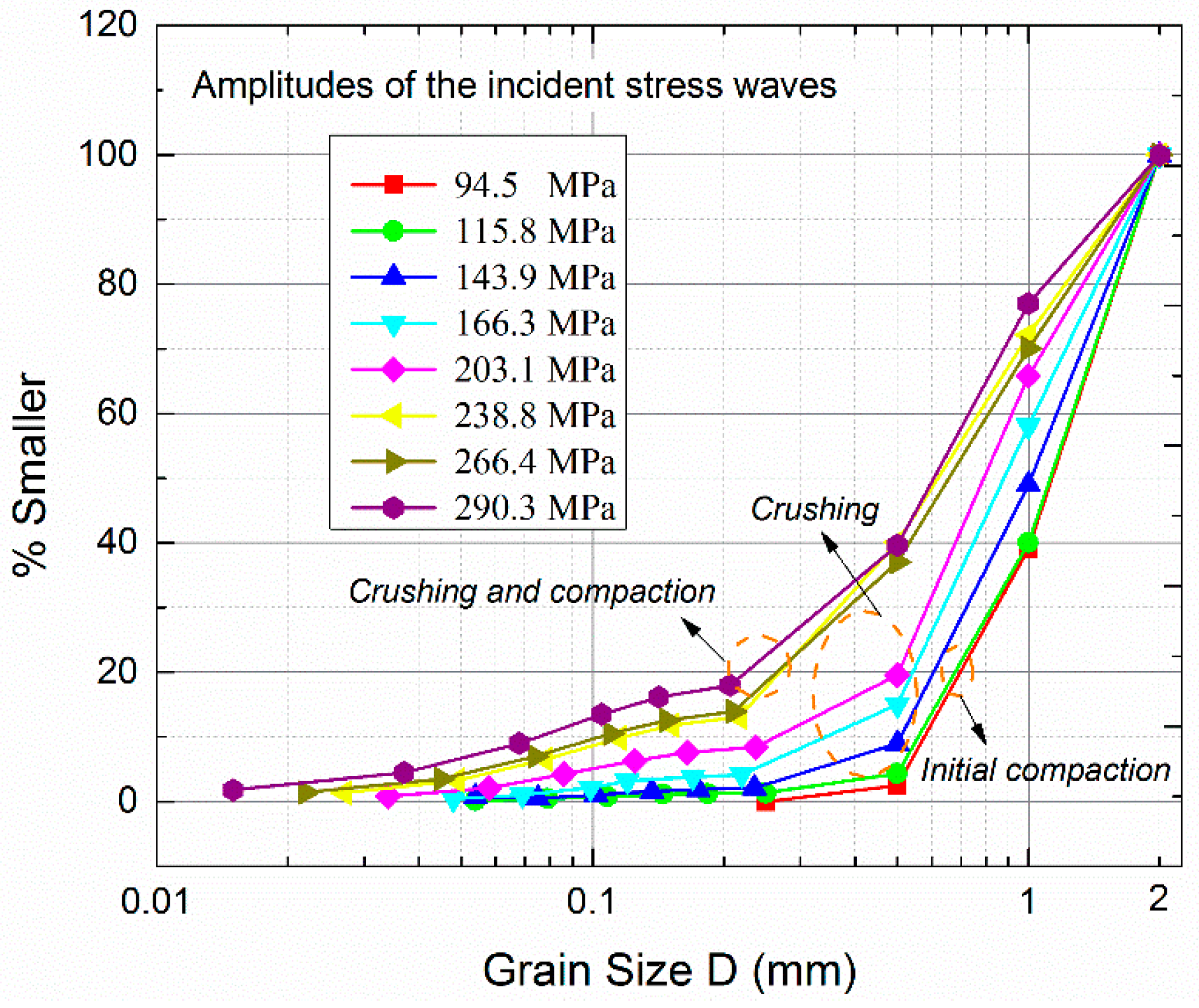
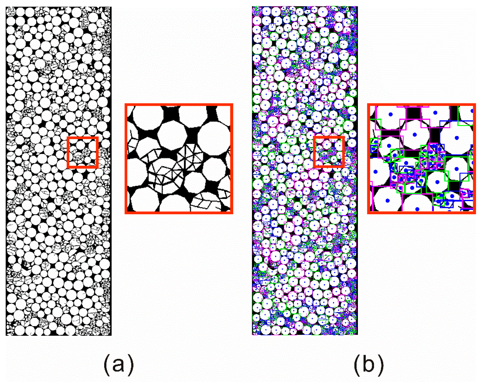
3.2. The Crush of Filled Particles and Its Effect on the Transmission Coefficient
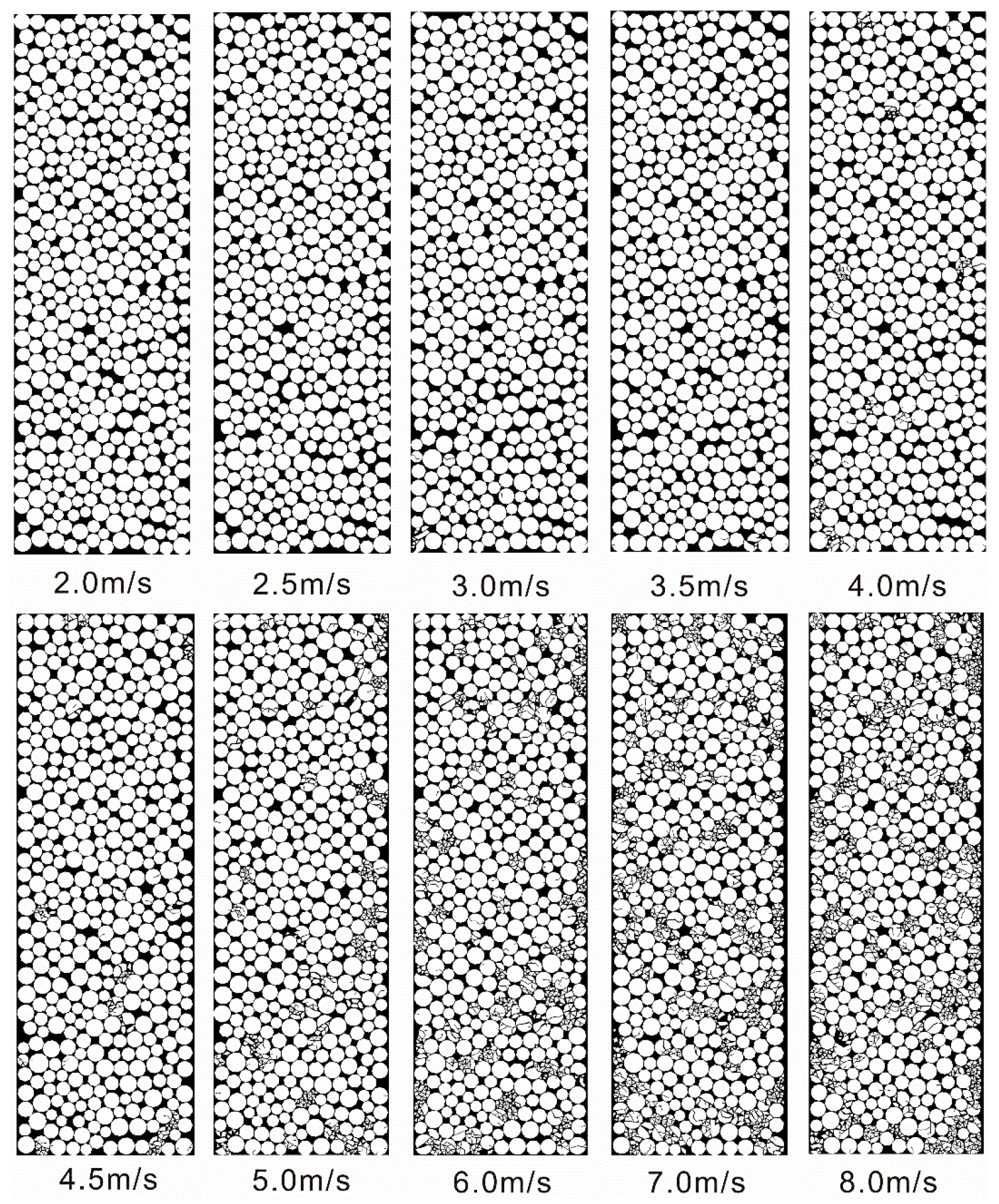
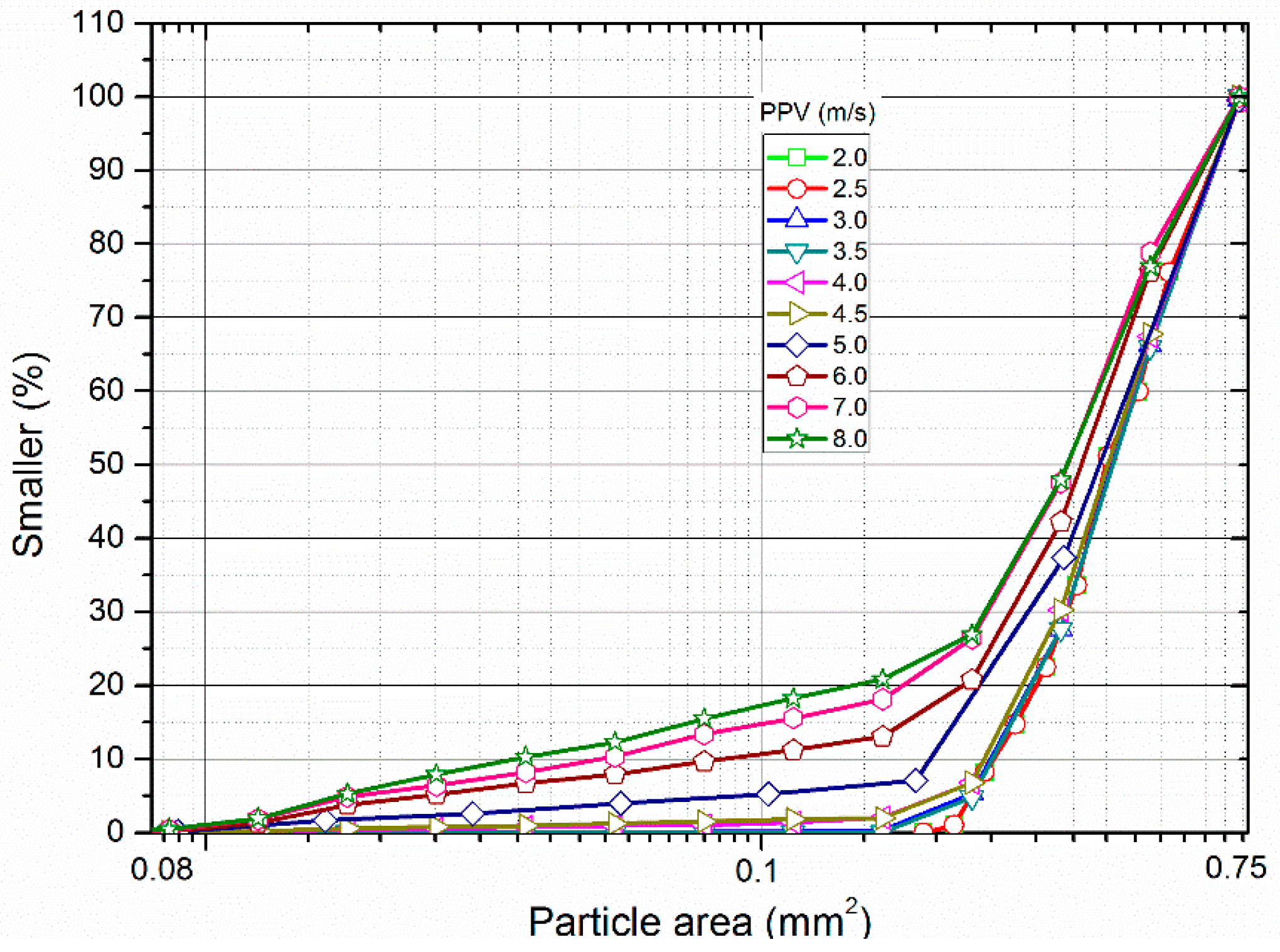
3.2.1. Influence of the PPV of the Incident Wave
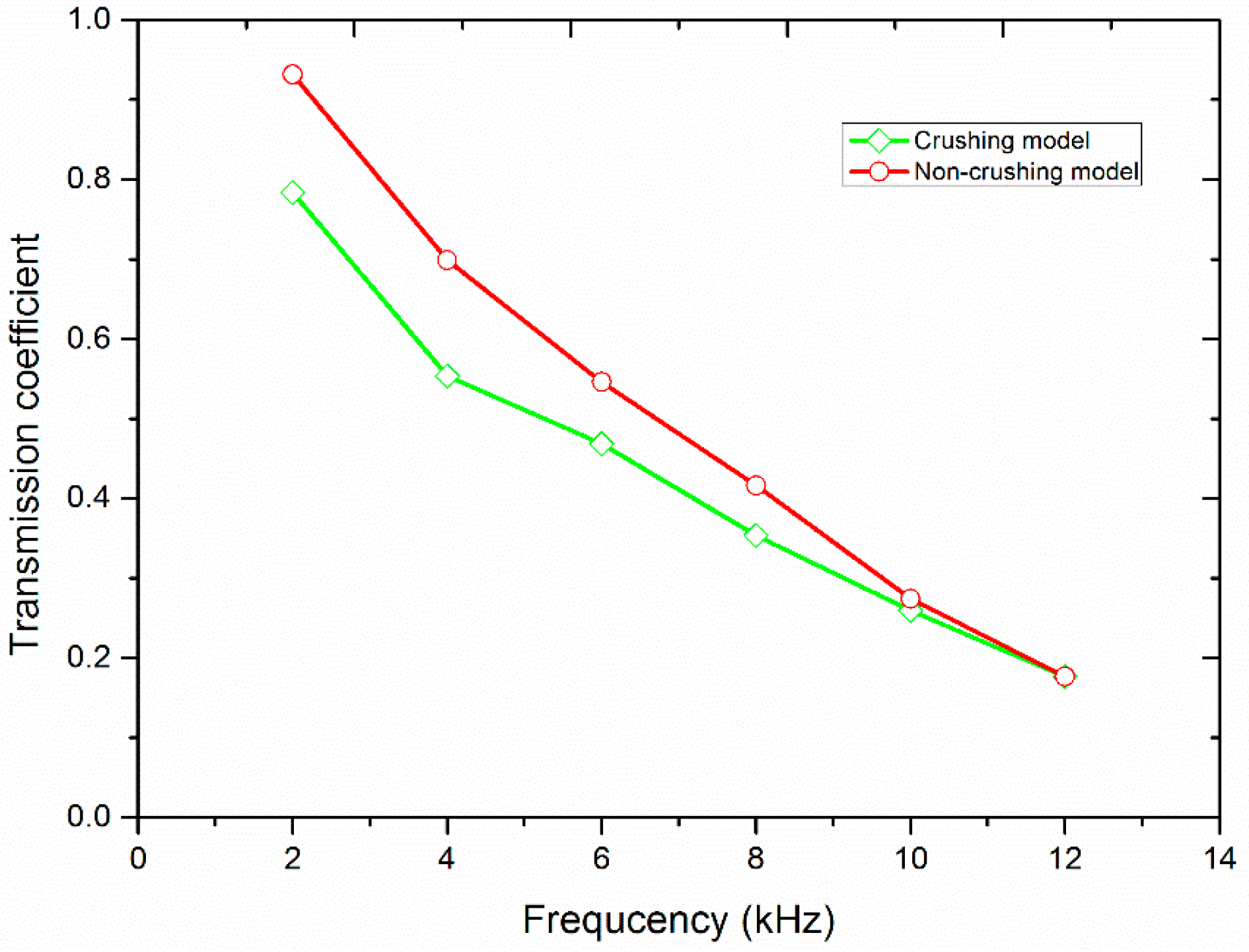
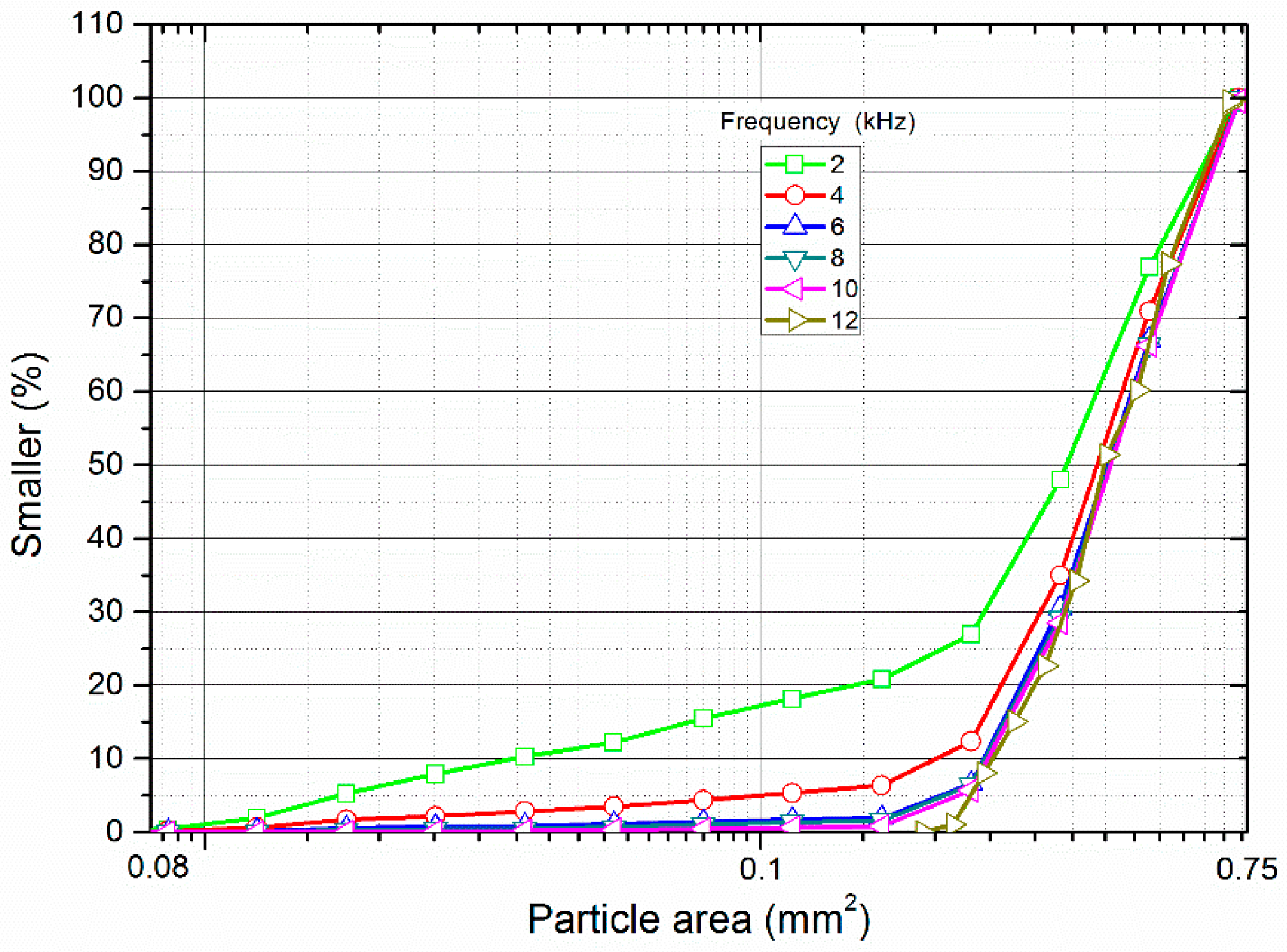
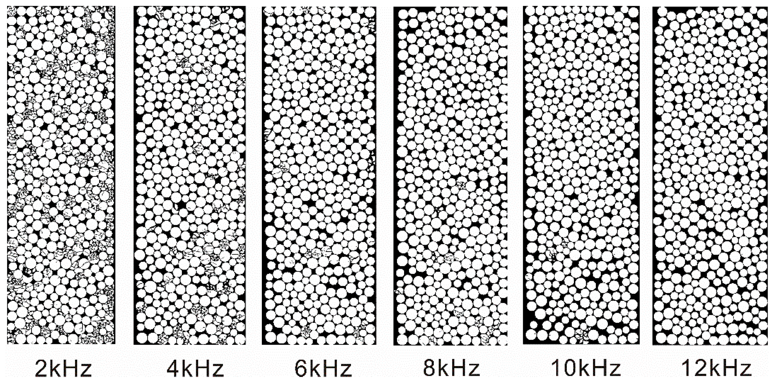
3.2.2. Influence of the Frequency of the Incident Wave
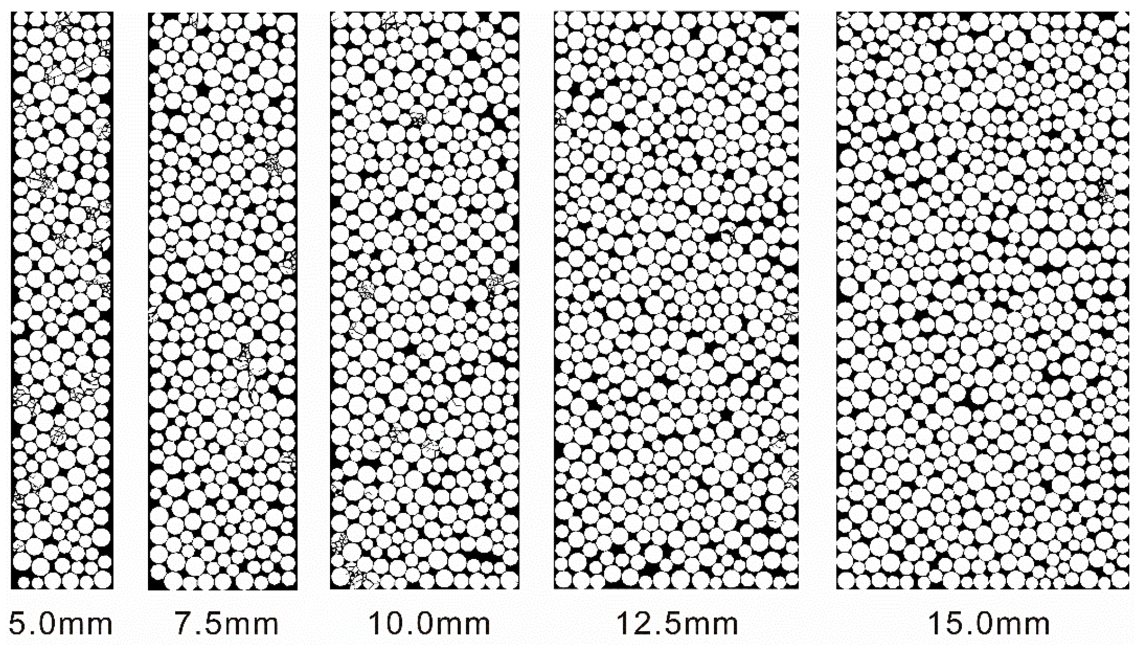
3.2.3. Influence of the Filled Thickness
4. Discussion
5. Conclusions
Acknowledgments
Author Contributions
Conflicts of Interest
References
- Goodman, R.E. Methods of Geological Engineering in Discontinuous Rocks; West Information Publishing Group: Eagan, MN, USA, 1976. [Google Scholar]
- Sun, G.Z. Rock Mass Structure Mechanics; Science Press: Beijing, China, 1988. (In Chinese) [Google Scholar]
- King, M.; Myer, L.; Rezowalli, J. Experimental studies of elastic-wave propagation in a columnar-jointed rock mass. Geophys. Prospect. 1986, 34, 1185–1199. [Google Scholar] [CrossRef]
- Gu, J.; Zhao, Z. Considerations of the discontinuous deformation analysis on wave propagation problems. Int. J. Numer. Anal. Methods Geomech. 2009, 33, 1449–1465. [Google Scholar] [CrossRef]
- Zhao, G.F.; Zhao, X.B.; Zhu, J.B. Application of the numerical manifold method for stress wave propagation across rock masses. Int. J. Numer. Anal. Methods Geomech. 2014, 38, 92–110. [Google Scholar] [CrossRef]
- Zhao, J.; Sun, L.; Zhu, J.B. Modelling p-wave transmission across rock fractures by particle manifold method (pmm). Geomech. Geoeng. 2012, 7, 175–181. [Google Scholar] [CrossRef]
- Zhu, J.B.; Zhao, G.F.; Zhao, X.B.; Zhao, J. Validation study of the distinct lattice spring model (DLSM) on p-wave propagation across multiple parallel joints. Comput. Geotech. 2011, 38, 298–304. [Google Scholar] [CrossRef]
- Cai, J.; Zhao, J. Effects of multiple parallel fractures on apparent attenuation of stress waves in rock masses. Int. J. Rock Mech. Min. Sci. 2000, 37, 661–682. [Google Scholar] [CrossRef]
- Chen, S.; Zhao, J. A study of udec modelling for blast wave propagation in jointed rock masses. Int. J. Rock Mech. Min. Sci. 1998, 35, 93–99. [Google Scholar] [CrossRef]
- De Lemos, J.A.S.V. A Distinct Element Model for Dynamic Analysis of Jointed Rock with Application to Dam Foundations and Fault Motion; University Microfilms: Ann Arbor, MI, USA, 1997. [Google Scholar]
- Resende, R.; Lamas, L.N.; Lemos, J.V.; Calçada, R. Micromechanical modelling of stress waves in rock and rock fractures. Rock Mech. Rock Eng. 2010, 43, 741–761. [Google Scholar] [CrossRef]
- Deng, X.F.; Zhu, J.B.; Chen, S.G.; Zhao, J. Some fundamental issues and verification of 3DEC in modeling wave propagation in jointed rock masses. Rock Mech. Rock Eng. 2012, 45, 943–951. [Google Scholar]
- Zhao, J.; Cai, J.G.; Zhao, X.B.; Li, H.B. Dynamic model of fracture normal behaviour and application to prediction of stress wave attenuation across fractures. Rock Mech. Rock Eng. 2007, 41, 671–693. [Google Scholar] [CrossRef]
- Zhao, X.B.; Zhao, J.; Cai, J.G.; Hefny, A.M. Udec modelling on wave propagation across fractured rock masses. Comput. Geotech. 2008, 35, 97–104. [Google Scholar] [CrossRef]
- Zhu, J.B.; Deng, X.F.; Zhao, X.B.; Zhao, J. A numerical study on wave transmission across multiple intersecting joint sets in rock masses with udec. Rock Mech. Rock Eng. 2012, 46, 1429–1442. [Google Scholar] [CrossRef]
- Barton, N. A Review of the Shear Strength of Filled Discontinuities in Rock; Norwegian Geotechnical Institute: Oslo, Norway, 1974. [Google Scholar]
- Sinha, U.; Singh, B. Testing of rock joints filled with gouge using a triaxial apparatus. Int. J. Rock Mech. Min. Sci. 2000, 37, 963–981. [Google Scholar] [CrossRef]
- Wu, W.; Li, J.C.; Zhao, J. Seismic response of adjacent filled parallel rock fractures with dissimilar properties. J. Appl. Geophys. 2013, 96, 33–37. [Google Scholar] [CrossRef]
- Zhu, J.B.; Perino, A.; Zhao, G.F.; Barla, G.; Li, J.C.; Ma, G.W.; Zhao, J. Seismic response of a single and a set of filled joints of viscoelastic deformational behaviour. Geophys. J. Int. 2011, 186, 1315–1330. [Google Scholar] [CrossRef]
- Li, J.C.; Ma, G.W. Experimental study of stress wave propagation across a filled rock joint. Int. J. Rock Mech. Min. Sci. 2009, 46, 471–478. [Google Scholar] [CrossRef]
- Wu, W.; Li, J.C.; Zhao, J. Loading rate dependency of dynamic responses of rock joints at low loading rate. Rock Mech. Rock Eng. 2012, 45, 421–426. [Google Scholar] [CrossRef]
- Huang, X.L.; Qi, S.W.; Williams, A.; Zou, Y.; Zheng, B.W. Numerical simulation of stress wave propagating through filled joints by particle model. Int. J. Solids Struct. 2015, 69, 23–33. [Google Scholar] [CrossRef]
- Xia, K.W.; Huang, S.; Marone, C. Laboratory observation of acoustic fluidization in granular fault gouge and implications for dynamic weakening of earthquake faults. Geochem. Geophys. Geosyst. 2013, 14, 1012–1022. [Google Scholar] [CrossRef]
- Khandelwal, M.; Singh, T. Evaluation of blast-induced ground vibration predictors. Soil Dynam. Earthq. Eng. 2007, 27, 116–125. [Google Scholar] [CrossRef]
- Singh, P.K. Blast vibration damage to underground coal mines from adjacent open-pit blasting. Int. J. Rock Mech. Min. Sci. 2002, 39, 959–973. [Google Scholar] [CrossRef]
- Omidvar, M.; Iskander, M.; Bless, S. Stress-strain behavior of sand at high strain rates. Int. J. Impact Eng. 2012, 49, 192–213. [Google Scholar] [CrossRef]
- Huang, X.; Qi, S.; Xia, K.; Zheng, H.; Zheng, B. Propagation of high amplitude stress waves through a filled artificial joint: An experimental study. J. Appl. Geophys. 2016, 130, 1–7. [Google Scholar] [CrossRef]
- Munjiza, A.; Owen, D.; Bicanic, N. A combined finite-discrete element method in transient dynamics of fracturing solids. Eng. Comput. 1995, 12, 145–174. [Google Scholar] [CrossRef]
- Lisjak, A.; Grasselli, G.; Vietor, T. Continuum–discontinuum analysis of failure mechanisms around unsupported circular excavations in anisotropic clay shales. Int. J. Rock Mech. Min. Sci. 2014, 65, 96–115. [Google Scholar] [CrossRef]
- Mahabadi, O.; Cottrell, B.; Grasselli, G. An example of realistic modelling of rock dynamics problems: Fem/dem simulation of dynamic brazilian test on barre granite. Rock Mech. Rock Eng. 2010, 43, 707–716. [Google Scholar] [CrossRef]
- Mahabadi, O.; Grasselli, G.; Munjiza, A. Y-GUI: A graphical user interface and pre-processor for the combined finite-discrete element code, Y2D, incorporating material heterogeneity. Comput. Geosci. 2010, 36, 241–252. [Google Scholar] [CrossRef]
- Mahabadi, O.; Lisjak, A.; Munjiza, A.; Grasselli, G. Y-geo: New combined finite-discrete element numerical code for geomechanical applications. Int. J. Geomech. 2012, 12, 676–688. [Google Scholar] [CrossRef]
- Zhao, Q.; Lisjak, A.; Mahabadi, O.; Liu, Q.; Grasselli, G. Numerical simulation of hydraulic fracturing and associated microseismicity using finite-discrete element method. J. Rock Mech. Geotech. Eng. 2014, 6, 574–581. [Google Scholar] [CrossRef]


| Parameters | Rock Bars (Granite) | Particles (Fused Quartz Sand) |
|---|---|---|
| Young’s modulus E (GPa) | 60.0 a | 72.0 c |
| Poisson’s ratio υ | 0.20 b | 0.17 c |
| Density ρ (kg/m3) | 2650.0 a | 2200.0 c |
| Friction coefficient of the intact material μi | 0.25 b | 0.25 b |
| Parameter | Value |
|---|---|
| Tensile strength ft (MPa) | 114 |
| Cohesion strength c (MPa) | 228 |
| Mode I fracture energy GI (J/m2) | 1250 |
| Mode II fracture energy GII (J/m2) | 2500 |
| Friction coefficient of the fracture μf | 0.5 |
| Normal contact penalty, pn (GPa/m) | 720 |
| Tangential contact penalty, pt (GPa/m) | 72 |
© 2016 by the authors. Licensee MDPI, Basel, Switzerland. This article is an open access article distributed under the terms and conditions of the Creative Commons Attribution (CC-BY) license ( http://creativecommons.org/licenses/by/4.0/).
Share and Cite
Huang, X.; Zhao, Q.; Qi, S.; Xia, K.; Grasselli, G.; Chen, X. Numerical Simulation on Seismic Response of the Filled Joint under High Amplitude Stress Waves Using Finite-Discrete Element Method (FDEM). Materials 2017, 10, 13. https://doi.org/10.3390/ma10010013
Huang X, Zhao Q, Qi S, Xia K, Grasselli G, Chen X. Numerical Simulation on Seismic Response of the Filled Joint under High Amplitude Stress Waves Using Finite-Discrete Element Method (FDEM). Materials. 2017; 10(1):13. https://doi.org/10.3390/ma10010013
Chicago/Turabian StyleHuang, Xiaolin, Qi Zhao, Shengwen Qi, Kaiwen Xia, Giovanni Grasselli, and Xuguang Chen. 2017. "Numerical Simulation on Seismic Response of the Filled Joint under High Amplitude Stress Waves Using Finite-Discrete Element Method (FDEM)" Materials 10, no. 1: 13. https://doi.org/10.3390/ma10010013