Article

Magnetic Anisotropy and Field‐induced Slow  Relaxation of Magnetization in Tetracoordinate CoII Compound [Co(CH3‐im)2Cl2]

1
Regional Centre of Advanced Technologies and Materials, Department of Inorganic Chemistry, Faculty of Science, Palacký University, 17. listopadu 12, CZ‐771 46 Olomouc, Czech Republic
2
Institute of Physical Chemistry, University of Stuttgart, Pfaffenwaldring 55, 70569 Stuttgart, Germany
*
Author to whom correspondence should be addressed.
Materials 2017, 10(3), 249; https://doi.org/10.3390/ma10030249
Submission received: 13 January 2017 / Accepted: 27 February 2017 / Published: 28 February 2017
(This article belongs to the Special Issue Advances in Molecular Magnets and related Phenomena)

Abstract

:
Static and dynamic magnetic properties of the tetracoordinate CoII complex [Co(CH3-im)2Cl2], (1, CH3-im = N-methyl-imidazole), studied using thorough analyses of magnetometry, and High-Frequency and -Field EPR (HFEPR) measurements, are reported. The study was supported by ab initio complete active space self-consistent field (CASSCF) calculations. It has been revealed that 1 possesses a large magnetic anisotropy with a large rhombicity (magnetometry: D = −13.5 cm−1, E/D = 0.33; HFEPR: D = −14.5(1) cm−1, E/D = 0.16(1)). These experimental results agree well with the theoretical calculations (D = −11.2 cm−1, E/D = 0.18). Furthermore, it has been revealed that 1 behaves as a field-induced single-ion magnet with a relatively large spin-reversal barrier (Ueff = 33.5 K). The influence of the Cl–Co–Cl angle on magnetic anisotropy parameters was evaluated using the CASSCF calculations.

Graphical Abstract

1. Introduction

Current interest in molecular compounds exhibiting magnetic blocking on a single molecule, so called single-molecule magnets (SMMs), lies in their potential practical applications in quantum computing or magnetic memories with a high density of storage [1]. The key parameter influencing static and dynamic magnetic properties of SMMs is represented by magnetic anisotropy, which manifests itself as a preferred direction of the spin, which may not be aligned with an external magnetic field, as promoted by the Zeeman Effect [2]. Two basic situations can be distinguished within the spin Hamiltonian formalism and described by the zero-field splitting (ZFS) parameters D (axial) and E (rhombic):
H ^ = D ( S ^ z 2 S ^ 2 / 3 ) + E ( S ^ x 2 S ^ y 2 )
(a) if the magnetization of the molecule exhibits a directional character, it is classified as uniaxial, containing an easy axis (D < 0); (b) if the character of magnetization is planar, the anisotropy is called easy-plane (D > 0) [3]. The value of the rhombic parameter must lie in the interval of E/D = 0−1/3 where the larger limiting value is considered as perfect rhombicity at which the sign of the D parameter cannot be determined experimentally. Furthermore, if D > 0 and if anisotropy is approaching perfect rhombicity, then magnetization is not of an easy-plane type anymore and it is strongly directional, but not along the z-axis. On the other hand, the magnetization of molecules with D < 0 stays axial even at E/D = 1/3 (Figure 1 left). The reason for this lies in the choice of the coordinate system for the components of the D-tensor (Dii). When the ideal rhombicity is achieved (or overpassed), the change of the canonical order of the D-tensor components occurs (for more detailed explanation, see the work of M. Atanasov et al. [4]). This is also reflected in a change of the magnetization axes without a change of the overall (orientationally averaged) magnetic properties (Figure 1 right).
The above mentioned considerations have significant consequences with respect to a definition of the spin reversal barrier (Ueff) of SMMs. The well-established relationship defines Ueff for integer spins (S) as Ueff = ǀDǀ × S2 and for non-integer spins as Ueff = ǀDǀ × (S2 − 1/4). It is clear that if one wants to increase the value of Ueff, there are only two possibilities: to increase the ground state spin or the absolute value of D. Previously, it was shown that increasing of total S by synthesizing large polynuclear clusters of paramagnetic metal atoms does not lead to increasing of Ueff. Furthermore, this strategy is not straightforward either from the synthetic or from theoretical point of view [5,6]. The other strategy involves deliberate tuning of magnetic anisotropy. Again, this is not straightforward for polynuclear complexes due to different mutual orientations of local D-tensor components depending on several conditions (e.g., cluster topology, differences in compositions of the coordination polyhedra implying different types of anisotropy) and interplay between the magnetic coupling and anisotropy [7]. Nevertheless, if we consider a special category of SMMs with one paramagnetic center, so called single-ion magnets (SIMs), then the deliberate modulation of the magnetic anisotropy is easier and depends reasonably on the topology and donor atom constitution of the coordination polyhedron [2]. Up to now, several correlations on the relationship between a structure and anisotropy parameters have been reported, namely for tetracoordinate [8,9], pentacoordinate [10,11], hexacoordinate NiII and CoII compounds [12,13], tetracoordinate FeII compounds [14] and penta and hexacoordinate MnIII compounds [15,16]. From these, the largest number of complexes exhibiting slow-relaxation of magnetization belongs undoubtedly to the group of tetracoordinate CoII compounds, which we have chosen as an object of the present study.
The ground electronic state in tetracoordinate CoII complexes (with S = 3/2) with the ideal Td geometry is 4A2 (the same for the C2v point group), but with lowering of the symmetry it might change to 4B1(D2d), 4A’’(CS) and 4A(C1). The ground state is split by ZFS in two Kramers doublets ǀ3/2,±3/2> and ǀ3/2,±1/2> and these two levels are separated by an energy difference equal to 2D. If the rhombic anisotropy is present, the distance between the Kramers doublets increases by 2√(D2 + 3E2). Usually, the tetracoordinate CoII compounds of the composition [Co(LN/P)2(L1)2], (where LN/P = a monodentate N/P-donor ligand, L1 = halogenido or pseudohalogenido ligands), adopt values of D parameters ranging from −14 to +6 cm−1 [17]. It must be noted that much larger values of D were observed for compounds involving monodentate ligands with soft donor atoms such as S or Se [18], bidentate N-donor ligands [19], and bidentate S/Se-donor ligands [20,21]. The aforementioned correlation [9] on the anisotropy of the [Co(LN/P)2(L1)2] compounds involves N/P-Co-N/P (α) and N/X-Co-N/X angles (β, N or X are the donor atoms from the L1 ligands) and it reads: δ = 2αTd – (α + β), where αTd is the angle of the ideal tetrahedron (109.5°). More negative/positive δ should lead to more negative/positive D. Thus, we performed a search in the CSD database (version 5.37 updated to May 2016) [22] for interesting candidates within the group of [Co(LN)2(Cl)2] compounds, which are readily synthetically available. Furthermore, in the previous works [9,17,23,24,25] the influence of the change in the α angle on D was well documented and therefore, we decided to study a compound with a large β angle, which should also lead to negative δ and D. From the CSD search we know that the average and median β values are both larger (114.1° and 114.4°) than the ideal tetrahedral angle. Therefore, we decided to choose to study the compound [Co(CH3-im)2Cl2], (1, CH3-im = N-methyl-imidazole), which possesses a relatively large β angle (117.9°) and to study its static and dynamic magnetic properties by Superconducting Quantum Interference Device (SQUID) magnetometry and High-Frequency and -Field EPR (HFEPR). Furthermore, we performed an extensive computational study of its electronic structure by CASSCF calculations and we studied the influence of widening of the β angle on the D and E parameters.

2. Results

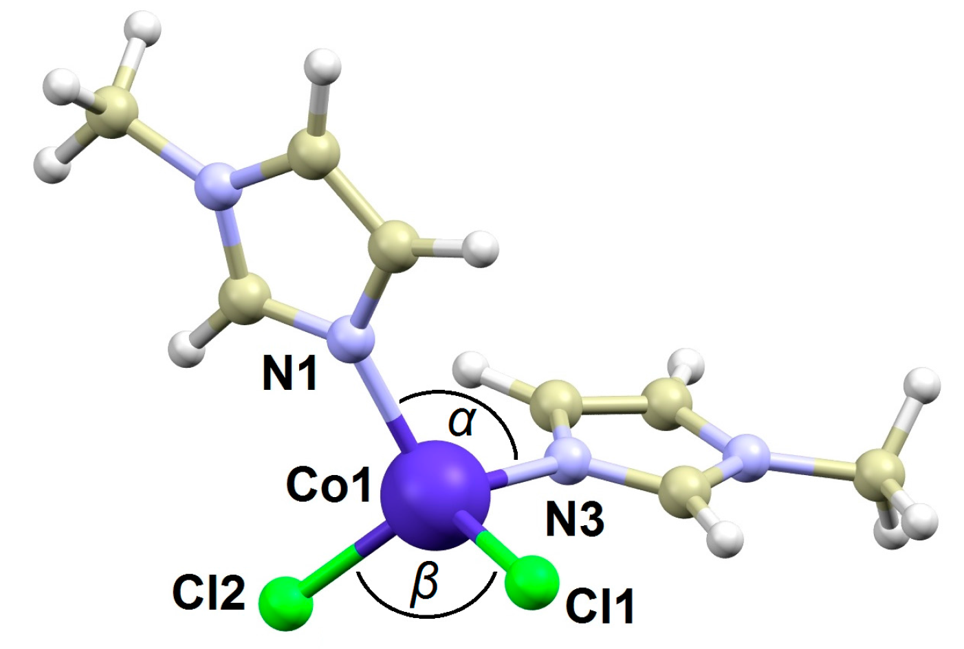
2.1. Crystal Structure

The crystal structure of the title compound 1 was reported in the year 2000 by S. Mukerjee et al. [26], but herein we will focus on the structural details, which might be important for the analysis of the magnetic behavior of this compound. The complex molecule in 1 is composed of two CH3-im and two Cl ligands coordinated to the CoII atom. As a result, the complex is tetracoordinate with symmetry of the coordination polyhedron close to C2v (Figure 2). The Co−N bonds are significantly shorter than the Co–Cl ones (in Å): d(Co−N) = 2.004(3) and 2.008(3), d(Co−Cl) = 2.2479(9) 2.2509(8). The Cl−Co−Cl angle is much wider than the N−Co−N one: <(Cl−Co−Cl) = 117.94(4)° and <(N−Co−N) = 110.6(1)°. Thus, the δ parameter is negative in this case (−9.5°).
The crystal structure of 1 does not contain any significant non-covalent contacts, only very weak C–H···Cl and C–H···π interactions are present. Furthermore, the shortest intermolecular Co···Co distance is 6.656(1) Å and thus, no mediation of magnetic exchange through non-covalent interactions or dipolar interaction can be expected. The phase identity of 1 was confirmed using powder X-ray diffraction and the observed powder diffraction pattern was compared to that calculated from the single-crystal data (Supplementary Materials, Figure S1).

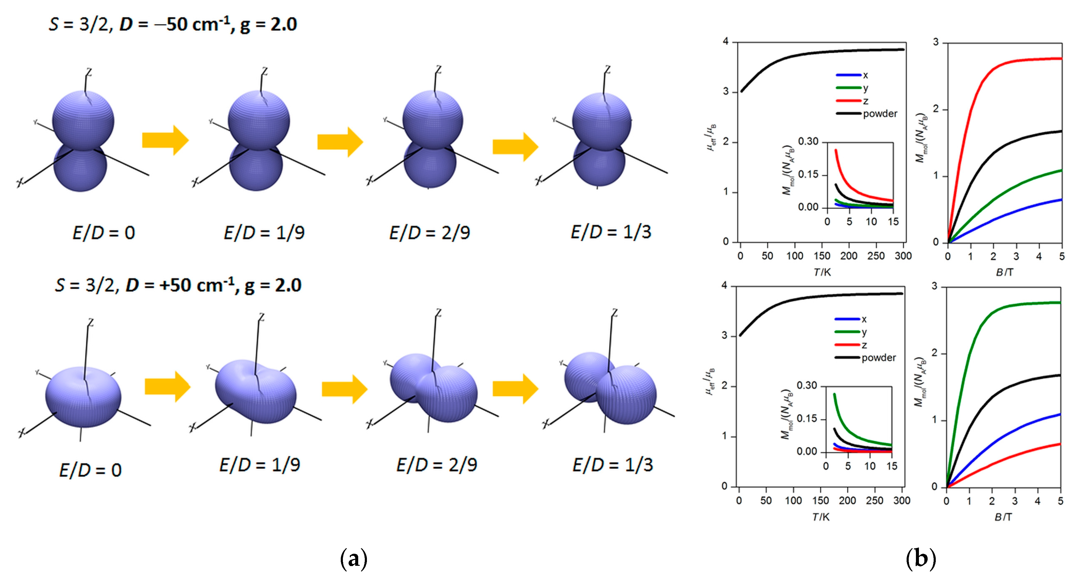
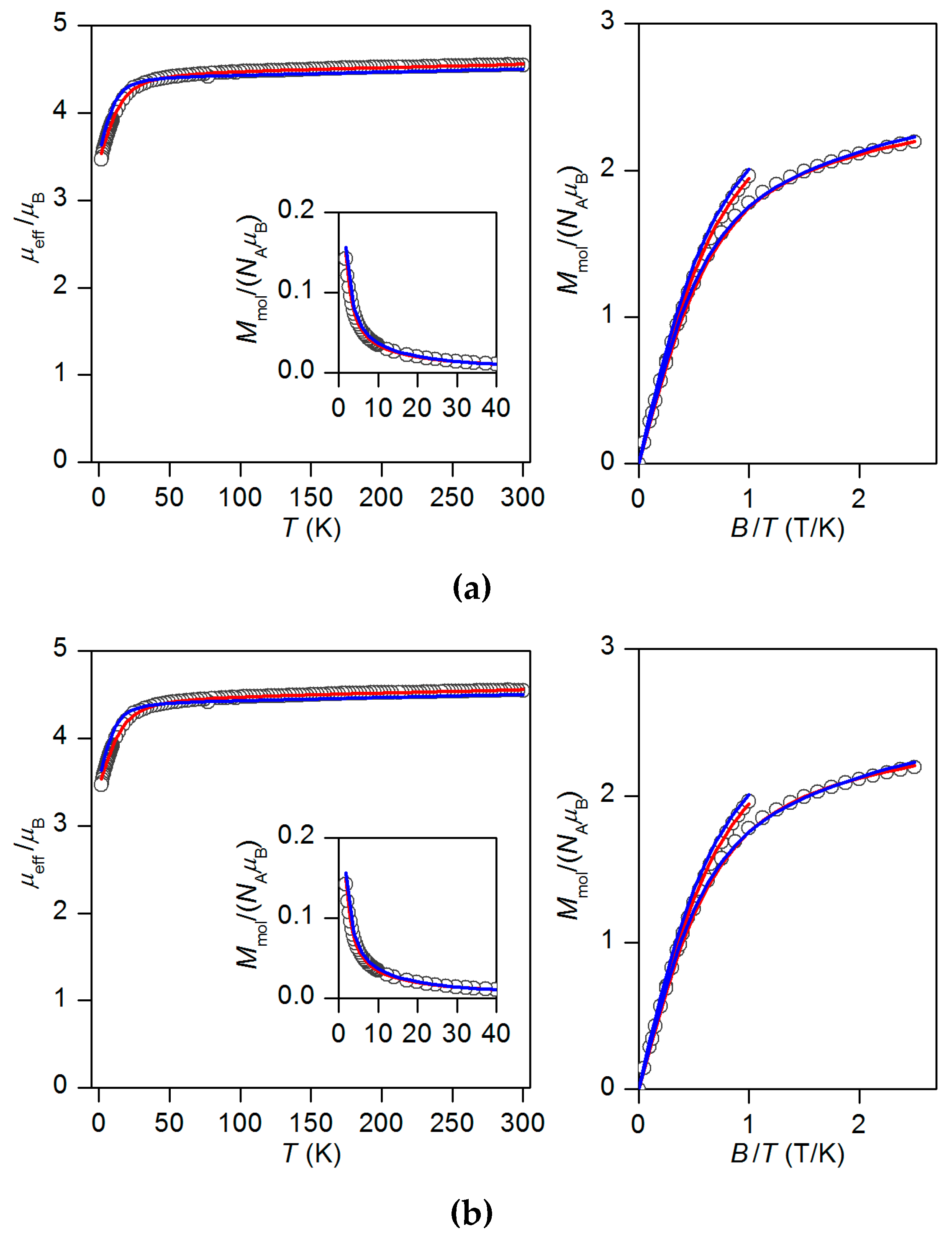
2.2. Static Magnetic Properties
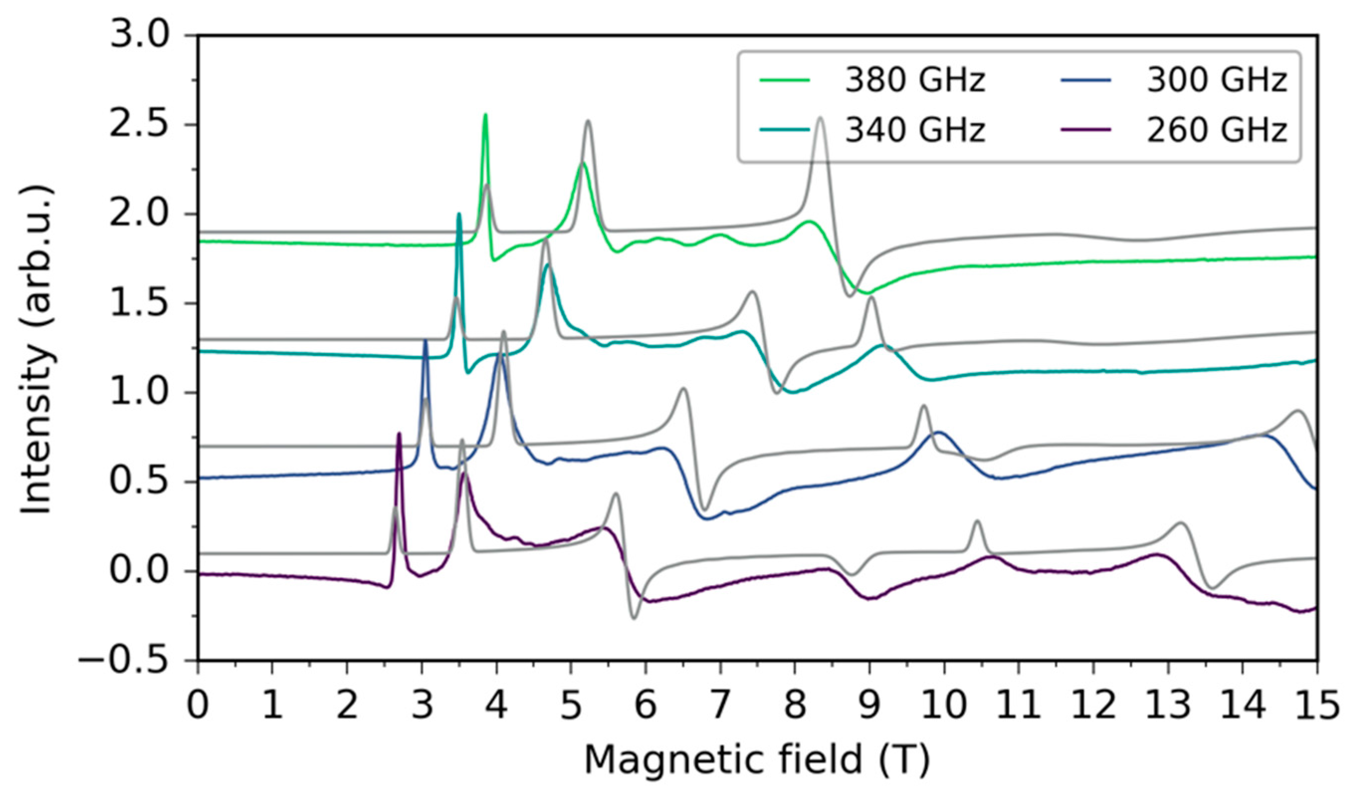
Temperature (1.9–300 K) and field (0–9 T) dependent magnetic data obtained by a physical property measurement system (PPMS) magnetometer are shown in Figure 3. The effective magnetic moment (μeff) at room temperature adopts the value of 4.4 μB. This value is significantly higher than the spin-only value for S = 3/2 and g = 2.0 (μeff/μB = 3.87) which directly indicates considerable contribution of a spin-orbit coupling to the ground state. Furthermore, μeff/μB starts to decrease on cooling below 40 K and it reaches the value of 3.5 at 1.9 K. From the field dependent measurements of molar magnetization it is clear that the isothermal magnetizations do not saturate to the value Mmol/NAμB = g × S. With respect to the mononuclear character of 1 and the absence of the intermolecular interactions capable of mediating magnetic exchange, such deviations from the ideal paramagnet behaviour cannot be explained by any other reasons than ZFS.
Thus, in order to analyze the magnetic properties of 1, we postulated the spin Hamiltonian for the monomeric complex including axial and rhombic terms of ZFS, and Zeeman term,
H ^ = D ( S ^ z 2 S ^ 2 / 3 ) + E ( S ^ x 2 S ^ y 2 ) + μ B B g S ^ a
where a defines the orientation of the magnetic field vector in polar coordinates as Ba = B(sin θ cos ϕ, sin θ sin ϕ, cos θ). The final calculated molar magnetization was calculated as an integral average in order to properly simulate the powder sample signal.
M mol = 1 / 4 π 0 2 π 0 π M a sin θ d θ d φ
Both, temperature- and field-dependent magnetic data were fitted simultaneously in order to find a reliable set of parameters. Firstly, the alternative with the negative D value was evaluated and the resulting fit is relatively good (Figure 3a) for D = −13.5 cm−1, E/D = 0.33, g = 2.287 and χTIP = 5.18 × 10⁻⁹ m3·mol−1, where χTIP stands for the contribution of temperature-independent paramagnetism [27]. Secondly, the positive D value was restrained in the fitting procedure and this resulted again in a very good fit, but with a little lower rhombicity: D = 14.3 cm−1, E/D = 0.30, g = 2.298 and χTIP = 5.04 × 10⁻⁹ m3·mol−1 (Figure 3b). Nevertheless, from the magnetic measurements it is clear that 1 has large rhombicity and we are not able to determine the sign of the D parameter unambiguously.

2.3. HFEPR

For a more accurate determination of the ZFS parameters we employed (HFEPR). Thus, spectra of pressed powder pellets were obtained at variable temperatures (from 8 to 40 K) and variable frequencies (from 100 to 500 GHz). The spectra were simulated on the basis of the spin Hamiltonian in the Equation (1) and we were able to reproduce all the dominant features observed in the simulations (Figure 4).
From the simulations, we found that the second rank axial ZFS parameter D = −14.5 ± 0.1 cm−1 is negative and similar in magnitude to that obtained from the PPMS measurements. However, the rhombicity is substantially lower: E/D = 0.16 ± 0.01. The g factor is anisotropic with gx = 2.21 ± 0.01, gy = 2.18 ± 0.01 and gz = 2.40 ± 0.01. Although most of the observed signals come from intradoublet transitions, the sign of D can be assigned unambiguously mainly due to the variable temperature measurements (Figures S9 and S10), which cannot be reproduced with a positive D. Further HFEPR measurements and analyses can be found in Supplementary Materials (Figures S2–S11).

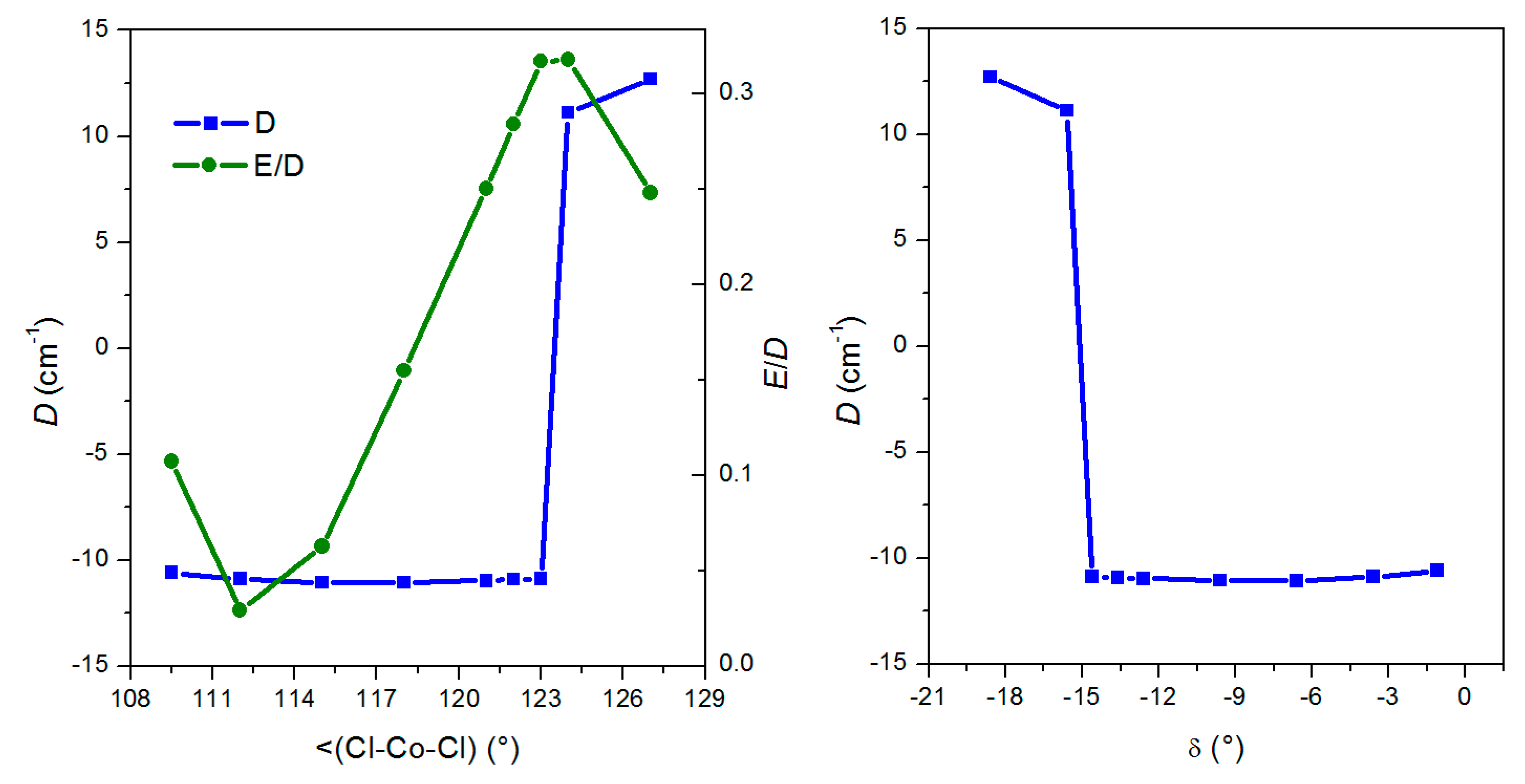
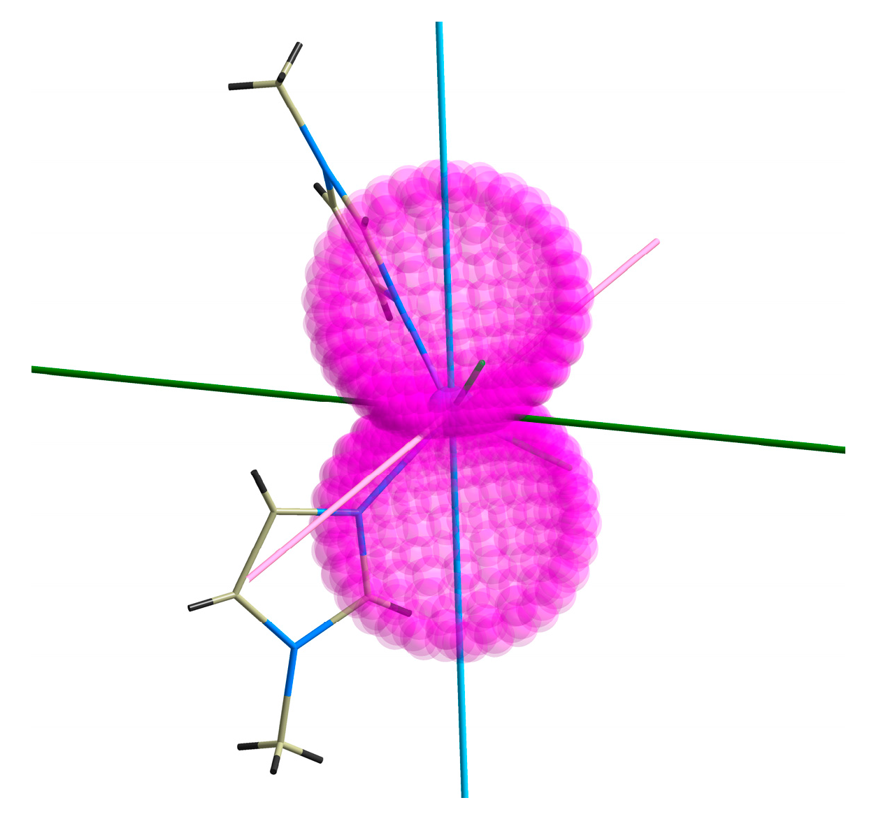
2.4. CASSCF Calculations

In order to support the analysis of the experimental data computationally we performed the complete active space self-consistent field (CASSCF) calculations complemented by N-electron valence second order perturbation theory (NEVPT2) using an ORCA 3.0 computational package [28]. The relativistic effects were included with a zero order regular approximation (ZORA) and scalar relativistic contracted version of def2-TZVP(-f) basis functions, as described in the Experimental Section 4.2.2. The spin Hamiltonian parameters were extracted with the help of the effective Hamiltonian theory. The resulting ZFS parameters for S = 3/2 are a little lower than those obtained from the HFEPR data: D = −11.2 cm−1, E/D = 0.18 (implying thus Ueff = 33.8 K/23.5 cm−1). The calculations also showed anisotropy of the g-tensor components (2.191, 2.240, 2.357, gav = 2.263), which agrees nicely with the results obtained by HFEPR. We also employed the respective ab initio CASSCF/NEVPT2 spin-orbit coupling, orbital and spin angular momentum matrices
H = H SOC + μ B ( L + g e S ) B
to calculate all 120 energy levels for any orientation of magnetic field Ba, followed by integral calculation of both temperature- and field-dependent magnetization data, which are in good agreement with the experimental data (Figure 3). Moreover, both lowest Kramers doublets (KD) were analyzed with the spin Hamiltonian for the effective spin Seff = 1/2, which resulted in the g-tensor components gKD1 = (1.051, 1.277, 6.850) and gKD2 = (2.152, 3.200, 5.430). Evidently, the lowest Kramers doublet has the axial type of the magnetic anisotropy, whereas the second Kramers doublet has a plane type of the magnetic anisotropy. Indeed, the easy axis type of the magnetic anisotropy is also clearly visible in Figure 5, where the 3D plot of the molar magnetization is overlaid over the molecular structure of 1 with the principle axes of the D-tensor.

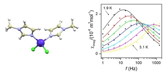
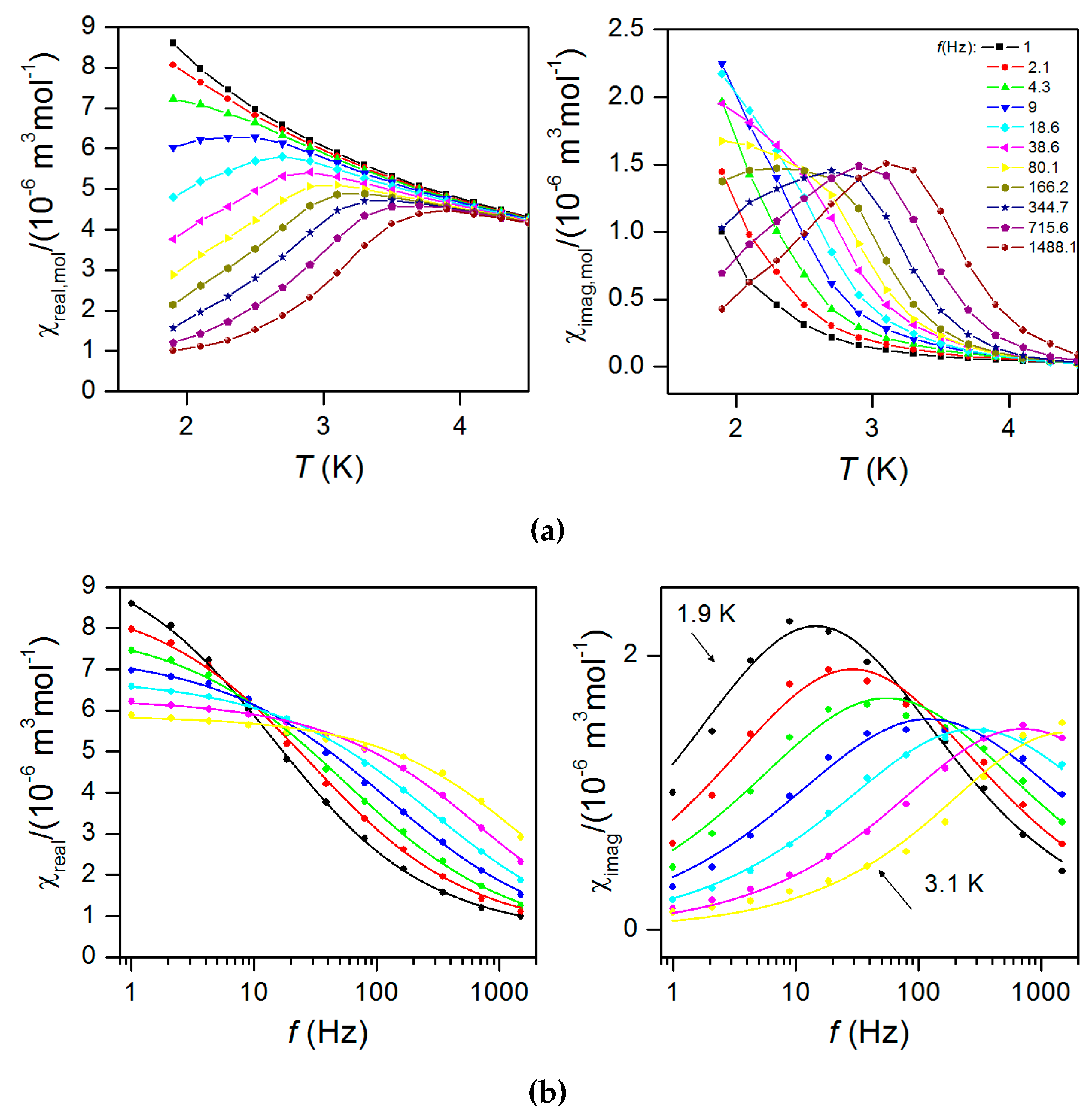
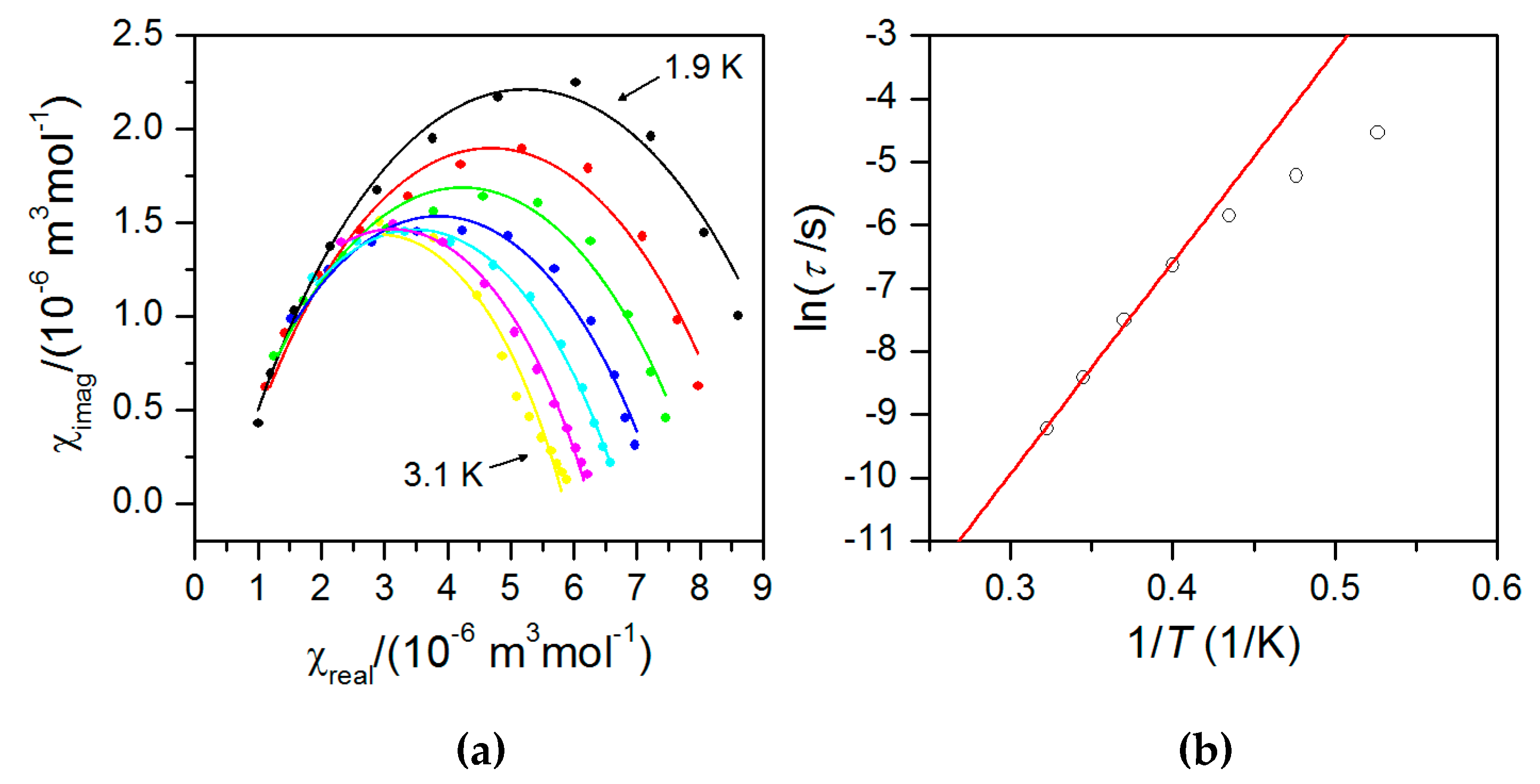
2.5. Dynamic Magnetic Properties

The AC susceptibility data measured in the zero static magnetic field showed no significant out-of-phase susceptibility signal (Supplementary Materials, Figure S12), but the field dependent measurement at T = 1.9 K confirmed field-induced slow relaxation of magnetization in 1 with a maximum at 0.2 T. This confirmed that 1 exhibits field-induced slow-relaxation of magnetization. Therefore, the AC data were collected at non-zero static field B = 0.2 T for various frequencies of small AC field as depicted in Figure 6. From this measurement it is obvious that the peak maxima are frequency dependent and 1 can be classified as field-induced SIM. Therefore, the analysis of the dynamic magnetic properties was done using the one-component Debye model:
χ(ω) = χS + (χTχS)/[1 + (iωτ)1−α]
As a result a set of parameters containing isothermal (χT) and adiabatic (χS) susceptibilities, relaxation times (τ) and distribution parameters (α) was obtained (Supplementary Materials, Table S1). Then, the Argand (Cole–Cole) plot (Figure 7) was constructed and using the Arrhenius expression for the temperature dependence of relaxation time resulted in τ0 = 2.11(0.95) × 10−9 s−1 and the spin reversal barrier Ueff = 33.5(1.2) K/23.3(0.8) cm−1 (Figure 7). Such derived value is slightly lower than the theoretical value of Ueff = 43.3 K/30.1 cm−1 estimated with D = −14.5 cm−1, E/D = 0.16, where the D and E values were determined by HFEPR. The reason why Ueff derived from the AC susceptibility data is smaller than theoretically predicted is that other relaxation processes than the Orbach one could also be present. However, the discrepancy can also be caused by the fact that with the Equation (5) only data having the maxima on the imaginary part of susceptibility are analyzed (T ≤ 3.1 K), and the non-zero values are already observed at ≈ 4 K. Therefore, we analysed these high temperature data for the highest frequencies with a simplified model derived under the assumption that the adiabatic susceptibility is usually approaching zero in the single-molecule magnets [29]
ln ( χ / χ ) = ln ( 2 π f τ 0 ) + U / k T
As a result, we obtained sets of the following parameters: τ0 = 1.8 × 10⁻¹⁰, Ueff = 29.8 cm−1 (42.9 K) for f = 1488.1 Hz, τ0 = 3.1× 10⁻¹⁰, Ueff = 28.5 cm−1 (41.0 K) for f = 715.6 Hz, τ0 = 4.2 × 10⁻¹⁰, Ueff = 28.2 cm−1 (40.6 K) for f = 344.7 Hz in Figure S13 (Supplementary Materials). The slight variation of the obtained parameters can be due to omitting the distribution of relaxation processes (parameter a in the Equation (5)). In this case Ueff is very close to the theoretical estimate ≈ 45 K.

3. Discussion

First, we will compare the results we obtained with the characteristics of the previously reported tetracoordinate compounds of the [Co(LN/P)2(L1)2] and [Co(LN/P)(L1)2] types. The values of the selected magnetic and structural parameters are listed in Table 1. Detailed inspection of the data and comparison with the correlation proposed by Boča and co-workers [9] show (Figure 8) that the relationship between δ and D is not linear, even if it is obvious that the compounds with negative δ tend to possess negative D and vice versa.
Next, as we mentioned in the introduction, the X–Co–X angle plays an important role in the above mentioned magneto-structural correlation. Furthermore, in this study, we have chosen the compound [Co(CH3-im)2Cl2] due to its relatively large Cl–Co–Cl angle (117.9°). From the structural data listed in Table 1, one can see that the X–Co–X angles are from a less extensive range of values (from 115.9° to 121.9°) in compounds with bidentate chelating ligands, while compounds with monodentate N/P-donor ligands adopt a much more variable range of the X–Co–X angles (from 108.3° to 121.4°). Therefore, we decided to explore the influence of the Cl–Co–Cl l angle on the ZFS parameters alone using the partially constrained geometry of the [Co(CH3-im)2Cl2] molecule with the Cl–Co–Cl angle adopting values close to the latter of the above-mentioned ranges. Thus, the N–Co–N angle was constrained to the value determined from the single-crystal X-ray diffraction experiment (110.6°) and the Cl–Co–Cl angle was varied from 109.5° to a maximal value of 127°. The molecular structure (for each Cl–Co–Cl angle) was optimized by DFT using PBE/ZORA/def2-TZVP(-f) including also dispersion correction (D3BJ) (see Section 4.2.2). As a result, we obtained a set of [Co(CH3-im)2Cl2] optimized molecular geometries with different Cl–Co–Cl angles and for each of them the CASSCF/NEVPT2 calculation was performed to deduce information about the D-tensors. The results of these calculations are shown in Figure 9.
It is clear that the change of the Cl-Co-Cl angle in the range from 109.5° to 123 has no significant influence on the D parameter, which is negative with a value close to −10.5 cm−1. Remarkably, in this region of the Cl-Co-Cl angle we see a dramatic increase in the rhombicity from E/D = 0.03 at 112° to almost perfect rhombicity (E/D = 0.32) at 124°. As a result, the change in the sign of the D parameter (Figure 9) is observed: D(at 124°) = 11.1 cm−1.. To sum up, no significant influence of the widening of the Cl-Co-Cl angle alone on the D value was predicted by the computational methods. On the other hand, the rhombicity parameter is strongly dependent on such widening to the extent that even a change of the D-sign at angles wider than 124° was predicted. Furthermore, it is evident that for the optimized geometries, the D-parameter does not correlate with the structural parameter δ (Figure 9). This, together with the above-mentioned discrepancy found for a set of magnetic and structural data for [Co(LN/P)2(L1)2] complexes, simply reveals that the previously proposed magneto-structural correlation [9] cannot cover all structural nuances in tetracoordinate CoII complexes.

4. Materials and Methods

4.1. Materials

All the starting chemicals were of analytical reagent grade and were used as received. All the chemicals were purchased from commercial sources (Sigma Aldrich, St. Louis, MO, USA).

Preparation of [Co(CH3-im)2Cl2]

A solution of CoCl2 (1 mmol, in 15 mL of methanol) was slowly added to a solution of N-methyl-imidazole (2 mmol, in 15 mL of methanol) during stirring. The solution immediately turned dark blue. It was stirred with heating for next 15 min and then it was filtered through a paper filter. After two days blue crystals formed and they were filtered off, washed with methanol and diethyether, dried and stored in a vacuum desiccator. Yield: 58%. Elem. anal. Calcd (%) for C8H12Cl2Co1N4: C, 32.68; H, 4.11; N, 19.05. Found: C, 32.77; H, 4.13; N, 18.75.

4.2. Methods

4.2.1. General Methods

Elemental analysis (CHN) was performed on a FLASH 2000 CHN Analyser (ThermoFisher Scientific, Waltham, MA, USA). The static magnetic data were measured on powdered samples pressed into pellets using a PPMS Dynacool (Quantum Design Inc., San Diego, CA, USA). The dynamic magnetic data were measured on powdered samples pressed into pellets stabilized by eicosane using a MPMS XL-7 Quantum Design SQUID magnetometer (Quantum Design Inc., San Diego, CA, USA). The experimental data were corrected for the diamagnetism of the constituent atoms by using Pascal's constants. The X-ray powder diffraction patterns were recorded on a Mini-Flex600 (Rigaku, Tokyo, Japan) instrument equipped with the Bragg–Brentano geometry, and with iron-filtered Cu Kα1,2 radiation. High-frequency EPR spectra were recorded on a home-built spectrometer. Its radiation source is a 0–20 GHz signal generator (Anritsu or VDI) in combination with an amplifier–multiplier chain (VDI) to obtain the required frequencies (80–1100 GHz). It features a quasi-optical bridge (Thomas Keating, Billingshurst, UK) and induction mode detection. The detector is a QMC Instruments magnetically tuned InSb hot electron bolometer. The sample is located in an Oxford Instruments 15/17 T cryomagnet equipped with a variable temperature insert (1.5–300 K). The spectrometer control program was written in LabView. The spectra were obtained on powdered samples pressed into pellets. A typical linewidth of a hyperfine-split Co line is around 3.4 mT, as can be seen for example in [37]. Due to inhomogeneous broadening of the lines (the narrowest of about 100 mT) in our spectra, the hyperfine interaction from the cobalt nucleus remained unresolved. HFEPR spectra were analyzed using the EasySpin [38] toolbox for MATLAB software.

4.2.2. Theoretical Methods

All theoretical calculations were performed with the ORCA 3.0 computational package [28]. All the calculations employed the scalar relativistic contracted version of def2-TZVP(-f) basis functions [39] together with the zero-order regular approximation (ZORA) [40,41]. The ZFS and g tensors were calculated by using self-consistent field (SA-CASSCF) wave functions [42] complemented by N-electron valence second-order perturbation theory (NEVPT2) [43]. The active space of the CASSCF calculation was set to five d-orbitals of CoII (CAS(7,5)). The ZFS parameters, based on dominant spin−orbit coupling contributions from excited states, were calculated through quasi-degenerate perturbation theory (QDPT) [44], in which approximations to the Breit–Pauli form of the spin-orbit coupling operator (SOMF approximation) [45] and the effective Hamiltonian theory [46] were utilized. The contributions of excited states to the ZFS terms are tabulated in Table S2 and the energy levels of ligand field multiplets are listed in Table S3. The DFT calculations were based on PBE functional [47] and dispersion correction (D3BJ) was also included [48].

Supplementary Materials

The following are available online at www.mdpi.com/1996-1944/10/3/249/s1. Figure S1: X-ray powder diffraction pattern for 1, Figure S2: HFEPR frequency dependence of 1 at 8 K, Figure S3: HFEPR frequency dependence of 1 at 13 K, Figure S4: HFEPR frequency dependence of 1 at 22 K, Figure S5: HFEPR temperature dependence of 1 at 260 GHz, Figure S6: HFEPR temperature dependence of 1 at 300 GHz, Figure S7: HFEPR temperature dependence of 1 at 340 GHz, Figure S8: HFEPR temperature dependence of 1 at 380 GHz, Figure S9: HFEPR frequency dependence of 1 at 8 K in the range from 100 to 500 GHz, Figure S10: HFEPR detail of variable temperature measurements and calculations at 380 GHz., Figure S11 Frequency/Field plot for the HFEPR measurements and calculations, Figure S12: The in-phase χreal and out-of-phase χimag molar susceptibilities for 1, Figure S13: Analysis of in-phase χreal and out-of-phase χimag molar susceptibilities for 1, Table S1: Parameters of one-component Debye model for 1, Table S2: The contributions of excited states to the ZFS terms, Table S3: The list of energy levels of ligand field multiplets.

Acknowledgments

We acknowledge financial support from the National Programme of Sustainability I (LO1305) of the Ministry of Education, Youth and Sports of the Czech Republic, and the Czech-German FP6-Mobility-9 project 7AMB15DE002. The authors thank Daniel Dvořák for his help with the preparation of the cobalt(II) complex.

Author Contributions

I.N., R.H., P.N. and Z.T. conceived and designed the experiments; I.N., R.H and P.N. performed the experiments; I.N., R.H. M.K., P.N., J.v.S. and Z.T. analyzed the data; I.N., R.H., M.K., P.N., J.v.S. and Z.T. wrote the paper. All authors read and approved the final manuscript.

Conflicts of Interest

The authors declare no conflict of interests.

References

  1. Ganzhorn, M.; Wernsdorfer, W. Molecular Magnets; Bartolome, J., Luis, F., Fernandez, J.F., Eds.; Springer: Berlin Heidelberg, Germany, 2014; pp. 319–364. [Google Scholar]
  2. Gómez-Coca, S.; Aravena, D.; Morales, R.; Ruiz, E. Large magnetic anisotropy in mononuclear metal complexes. Coord. Chem Rev. 2015, 289–290, 379–392. [Google Scholar] [CrossRef]
  3. Boča, R. Zero-field splitting in metal complexes. Coord. Chem Rev. 2004, 248, 757–815. [Google Scholar] [CrossRef]
  4. Atanasov, M.; Aravena, D.; Suturina, E.; Bill, E.; Maganas, D.; Neese, F. First principles approach to the electronic structure, magnetic anisotropy and spin relaxation in mononuclear 3d-transition metal single molecule magnets. Coord. Chem Rev. 2015, 289–290, 177–214. [Google Scholar] [CrossRef]
  5. Waldmann, O. A criterion for the anisotropy barrier in single-molecule magnets. Inorg. Chem. 2007, 46, 10035–10037. [Google Scholar] [CrossRef] [PubMed]
  6. Neese, F.; Pantazis, D.A. What is not required to make a single molecule magnet. Farad. Discuss. 2011, 148, 229–238; discussion 299–314. [Google Scholar] [CrossRef]
  7. Herchel, R.; Nemec, I.; Machata, M.; Trávníček, Z. Solvent-induced structural diversity in tetranuclear Ni(II) schiff-base complexes: The first Ni4 single-molecule magnet with a defective dicubane-like topology. Dalton Trans. 2016, 45, 18622–18634. [Google Scholar] [CrossRef] [PubMed]
  8. Jiang, S.-D.; Maganas, D.; Levesanos, N.; Ferentinos, E.; Haas, S.; Thirunavukkuarasu, K.; Krzystek, J.; Dressel, M.; Bogani, L.; Neese, F.; et al. Direct observation of very large zero-field splitting in a tetrahedral niiise4 coordination complex. J. Am. Chem. Soc. 2015, 137, 12923–12928. [Google Scholar] [CrossRef] [PubMed]
  9. Titiš, J.; Miklovič, J.; Boča, R. Magnetostructural study of tetracoordinate cobalt(II) complexes. Inorg. Chem. Comm. 2013, 35, 72–75. [Google Scholar] [CrossRef]
  10. Nemec, I.; Herchel, R.; Svoboda, I.; Boca, R.; Trávníček, Z. Large and negative magnetic anisotropy in pentacoordinate mononuclear Ni(II) Schiff base complexes. Dalton Trans. 2015, 44, 9551–9560. [Google Scholar] [CrossRef] [PubMed]
  11. Nemec, I.; Liu, H.; Herchel, R.; Zhang, X.; Trávníček, Z. Magnetic anisotropy in pentacoordinate 2,6-bis(arylazanylidene-1-chloromethyl)pyridine cobalt(II) complexes with chlorido co-ligands. Synth. Met. 2016, 215, 158–163. [Google Scholar] [CrossRef]
  12. Titiš, J.; Boča, R. Magnetostructural d correlation in nickel(II) complexes: Reinvestigation of the zero-field splitting. Inorg. Chem. 2010, 49, 3971–3973. [Google Scholar] [CrossRef] [PubMed]
  13. Titiš, J.; Boča, R. Magnetostructural d correlations in hexacoordinated cobalt(II) complexes. Inorg. Chem. 2011, 50, 11838–11845. [Google Scholar] [CrossRef] [PubMed]
  14. Werncke, C.G.; Bouammali, M.-A.; Baumard, J.; Suaud, N.; Martins, C.; Guihéry, N.; Vendier, L.; Zheng, J.; Sortais, J.-B.; Darcel, C.; et al. Ising-type magnetic anisotropy and slow relaxation of the magnetization in four-coordinate amido-pyridine Fe(II) complexes. Inorg. Chem. 2016, 55, 10968–10977. [Google Scholar] [CrossRef] [PubMed]
  15. Nemec, I.; Herchel, R.; Trávníček, Z. Pentacoordinate and hexacoordinate Mn(III) complexes of tetradentate schiff-base ligands containing tetracyanidoplatinate(II) bridges and revealing uniaxial magnetic anisotropy. Molecules 2016, 21, 1681. [Google Scholar] [CrossRef] [PubMed]
  16. Maurice, R.; de Graaf, C.; Guihéry, N. Magnetostructural relations from a combined ab initio and ligand field analysis for the nonintuitive zero-field splitting in Mn(III) complexes. J. Chem. Phys. 2010, 133, 084307. [Google Scholar] [CrossRef] [PubMed]
  17. Nemec, I.; Herchel, R.; Trávníček, Z. Suppressing of slow magnetic relaxation in tetracoordinate Co(II) field-induced single-molecule magnet in hybrid material with ferromagnetic barium ferrite. Sci. Rep. 2015, 5, 10761. [Google Scholar] [CrossRef] [PubMed]
  18. Zadrozny, J.M.; Telser, J.; Long, J.R. Slow magnetic relaxation in the tetrahedral cobalt(II) complexes [Co(EPh)4]2− (E=O, S, Se). Polyhedron 2013, 64, 209–217. [Google Scholar] [CrossRef]
  19. Rechkemmer, Y.; Breitgoff, F.D.; van der Meer, M.; Atanasov, M.; Hakl, M.; Orlita, M.; Neugebauer, P.; Neese, F.; Sarkar, B.; van Slageren, J. A four-coordinate cobalt(II) single-ion magnet with coercivity and a very high energy barrier. Nat. Commun. 2016, 7, 10467. [Google Scholar] [CrossRef] [PubMed]
  20. Fataftah, M.S.; Zadrozny, J.M.; Rogers, D.M.; Freedman, D.E. A mononuclear transition metal single-molecule magnet in a nuclear spin-free ligand environment. Inorg. Chem. 2014, 53, 10716–10721. [Google Scholar] [CrossRef] [PubMed]
  21. Sottini, S.; Poneti, G.; Ciattini, S.; Levesanos, N.; Ferentinos, E.; Krzystek, J.; Sorace, L.; Kyritsis, P. Magnetic anisotropy of tetrahedral coii single-ion magnets: Solid-state effects. Inorg. Chem. 2016, 55, 9537–9548. [Google Scholar] [CrossRef] [PubMed]
  22. Allen, F.H. The Cambridge Structural Database: A quarter of a million crystal structures and rising. Acta Cryst. 2002, B58, 380–388. [Google Scholar] [CrossRef]
  23. Smolko, L.; Černák, J.; Dušek, M.; Miklovič, J.; Titiš, J.; Boča, R. Three tetracoordinate co(ii) complexes [Co(biq)X2] (X = Cl, Br, I) with easy-plane magnetic anisotropy as field-induced single-molecule magnets. Dalton Trans. 2015, 44, 17565–17571. [Google Scholar] [CrossRef] [PubMed]
  24. Mondal, A.K.; Parmar, V.S.; Biswas, S.; Konar, S. Tetrahedral mii based binuclear double-stranded helicates: Single-ion-magnet and fluorescence behaviour. Dalton Trans. 2016, 45, 4548–4557. [Google Scholar] [CrossRef] [PubMed]
  25. Ziegenbalg, S.; Hornig, D.; Görls, H.; Plass, W. Cobalt(ii)-based single-ion magnets with distorted pseudotetrahedral [n2o2] coordination: Experimental and theoretical investigations. Inorg. Chem. 2016, 55, 4047–4058. [Google Scholar] [CrossRef] [PubMed]
  26. Mukerjee, S.; Skogerson, K.; DeGala, S.; Caradonna, J.P. Skirting the oxo-wall: Characterization and catalytic reactivity of binuclear Co2+/3+ 1,2-bis(2-hydroxybenzamido)benzene complexes with comparison to their isostructural Fe2+/3+ analogs. Implications of d-electron count on oxygen atom transfer catalysis. Inorg. Chim. Acta 2000, 297, 313–329. [Google Scholar] [CrossRef]
  27. Boča, R. Theoretical Foundations of Molecular Magnetism; Elsevier: Amsterdam, The Netherlands, 1999. [Google Scholar]
  28. Neese, F. The ORCA program system. Wiley Interdiscip. Rev.-Comput. Mol. Sci. 2012, 2, 73–78. [Google Scholar] [CrossRef]
  29. Antal, P.; Drahoš, B.; Herchel, R.; Trávníček, Z. Late first-row transition-metal complexes containing a 2-pyridylmethyl pendant-armed 15-membered macrocyclic ligand. Field-induced slow magnetic relaxation in a seven-coordinate cobalt(II) compound. Inorg. Chem. 2016, 55, 5957–5972. [Google Scholar] [CrossRef] [PubMed]
  30. Yang, F.; Zhou, Q.; Zhang, Y.; Zeng, G.; Li, G.; Shi, Z.; Wang, B.; Feng, S. Inspiration from old molecules: Field-induced slow magnetic relaxation in three air-stable tetrahedral cobalt(II) compounds. Chem. Commun. 2013, 49, 5289–5291. [Google Scholar] [CrossRef] [PubMed]
  31. Boča, R.; Miklovič, J.; Titiš, J. Simple mononuclear cobalt(II) complex: A single-molecule magnet showing two slow relaxation processes. Inorg. Chem. 2014, 53, 2367–2369. [Google Scholar] [CrossRef] [PubMed]
  32. Saber, M.R.; Dunbar, K.R. Ligands effects on the magnetic anisotropy of tetrahedral cobalt complexes. Chem. Commun. 2014, 50, 12266–12269. [Google Scholar] [CrossRef] [PubMed]
  33. Idešicová, M.; Titiš, J.; Krzystek, J.; Boča, R. Zero-field splitting in pseudotetrahedral Co(II) complexes: A magnetic, high-frequency and -field epr, and computational study. Inorg. Chem. 2013, 52, 9409–9417. [Google Scholar] [CrossRef] [PubMed]
  34. Rajnák, C.; Packová, A.; Titiš, J.; Miklovič, J.; Moncol’, J.; Boča, R. A tetracoordinate Co(II) single molecule magnet based on triphenylphosphine and isothiocyanato group. Polyhedron 2016, 110, 85–92. [Google Scholar] [CrossRef]
  35. Huang, W.; Liu, T.; Wu, D.; Cheng, J.; Ouyang, Z.W.; Duan, C. Field-induced slow relaxation of magnetization in a tetrahedral Co(II) complex with easy plane anisotropy. Dalton Trans. 2013, 42, 15326–15331. [Google Scholar] [CrossRef] [PubMed]
  36. Smolko, L.; Cernak, J.; Dusek, M.; Titiš, J.; Boča, R. Tetracoordinate Co(II) complexes containing bathocuproine and single molecule magnetism. New J. Chem. 2016, 40, 6593–6598. [Google Scholar] [CrossRef]
  37. Maganas, D.; Milikisyants, S.; Rijnbeek, J.M.A.; Sottini, S.; Levesanos, N.; Kyritsis, P.; Groenen, E.J.J. A multifrequency high-field electron paramagnetic resonance study of coiis4 coordination. Inorg. Chem. 2010, 49, 595–605. [Google Scholar] [CrossRef] [PubMed]
  38. Stoll, S.; Schweiger, A. EasySpin, a comprehensive software package for spectral simulations and analysis in EPR. J. Magn. Reson. 2006, 178, 42–55. [Google Scholar] [CrossRef] [PubMed]
  39. Pantazis, D.A.; Chen, X.-Y.; Landis, C.R.; Neese, F. All-Electron Scalar Relativistic Basis Sets for Third-Row Transition Metal Atoms. J. Chem. Theory Comput. 2008, 4, 908–919. [Google Scholar] [CrossRef] [PubMed]
  40. van Lenthe, E.; Baerends, E.J.; Snijders, J.G. Relativistic regular two-component Hamiltonians. J. Chem. Phys. 1993, 99, 4597–4610. [Google Scholar] [CrossRef]
  41. Van Wüllen, C. Molecular density functional calculations in the regular relativistic approximation: Method, application to coinage metal diatomics, hydrides, fluorides and chlorides, and comparison with first-order relativistic calculations. J. Chem. Phys. 1998, 109, 392–399. [Google Scholar] [CrossRef]
  42. Malmqvist, P.-Å.; Roos, B.O. The CASSCF state interaction method. Chem. Phys. Lett. 1989, 155, 189–194. [Google Scholar] [CrossRef]
  43. Angeli, C.; Cimiraglia, R.; Evangelisti, S.; Leininger, T.; Malrieu, J.P. Introduction of n-electron valence states for multireference perturbation theory. J. Chem. Phys. 2001, 114, 10252–10264. [Google Scholar] [CrossRef]
  44. Ganyushin, D.; Neese, F. First-principles calculations of zero-field splitting parameters. J. Chem. Phys. 2006, 125, 024103. [Google Scholar] [CrossRef] [PubMed]
  45. Neese, F. Efficient and accurate approximations to the molecular spin-orbit coupling operator and their use in molecular g-tensor calculations. J. Chem. Phys. 2005, 122, 034107. [Google Scholar] [CrossRef] [PubMed]
  46. Maurice, R.; Bastardis, R.; de Graaf, C.; Suaud, N.; Mallah, T.; Guihéry, N. Universal Theoretical Approach to Extract Anisotropic Spin Hamiltonians. J. Chem. Theory Comput. 2009, 5, 2977–2984. [Google Scholar] [CrossRef] [PubMed]
  47. Perdew, J.P.; Burke, K.; Ernzerhof, M. Generalized gradient approximation made simple. Phys. Rev. Lett. 1996, 77, 3865–3868. [Google Scholar] [CrossRef] [PubMed]
  48. Grimme, S.; Antony, J.; Ehrlich, S.; Krieg, H. A consistent and accurate ab initio parametrization of density functional dispersion correction (dft-d) for the 94 elements h-pu. J. Chem. Phys. 2010, 132, 154104. [Google Scholar] [CrossRef] [PubMed]
Figure 1. (a) The 3D visualization of the molar magnetization calculated at T = 2 K and B = 3 T for S = 3/2 with various D and E parameters as indicated in the plot. (b) The effective magnetic moment with molar magnetization in the inset (B = 0.1 T) and the isothermal magnetization at T = 2 K calculated for D = −50 cm−1, E/D = 1/3 (top) and D = +50 cm−1, E/D = 1/3 (bottom).
Materials 10 00249 g001
Figure 2. Molecular structure of 1. Selected bond lengths (in Å) and angles (in °): d(Co1−N1) = 2.004(3), d(Co1−N3) = 2.008(3), d(Co1−Cl1) = 2.2509(8), d(Co1−Cl2) = 2.2479(9), <(Cl1−Co1−Cl2, α angle) = 117.94(4), <(N1−Co−N3, β angle) = 110.6(1), <(N1−Co−Cl2) = 103.42(8), <(N1−Co−Cl1) = 111.08(8), <(N3−Co−Cl1) = 105.52(8), <(N3−Co−Cl2) = 108.26(9). The X-ray data were adapted from CSD refcode XIWKIX [22].
Materials 10 00249 g002
Figure 3. The magnetic data for 1 depicted as temperature dependence of the effective magnetic moment calculated from the molar magnetization measured at B = 0.1 T shown in the inset and reduced magnetization data measured at T = 2 and 5 K. Experimental data are depicted as empty circles, fitted data are shown as red lines. (a) The best fit for negative D: g = 2.287, D = −13.5 cm−1, E/D = 0.33 and χTIP = 5.18 × 10⁻⁹ m3·mol−1. (b) The best fit for positive D: g = 2.298, D = 14.3 cm−1, E/D = 0.30 and χTIP = 5.04 × 10⁻⁹ m3·mol−1. Blue lines correspond to magnetic data derived from CASSCF/NEVPT2 calculation.
Materials 10 00249 g003
Figure 4. HFEPR frequency dependence of 1 at 40 K. Colored lines represent experimental data, while grey lines represent the simulated spectra.
Materials 10 00249 g004
Figure 5. The CASSCF/NEVPT2 calculated principal axes of the D-tensor labeled DX (pink), DY (green), DZ (blue) visualized together with molecular structure of 1 and overlaid with calculated molar magnetization (B = 3 T, T = 2 K).
Materials 10 00249 g005
Figure 6. (a) In-phase χreal (left) and out-of-phase χimag (right) molar susceptibilities for 1 at the applied external field Bdc = 0.2 T. Lines serve as guides to the eyes. (b): Frequency dependence of in-phase χreal (left) and out-of-phase χimag (right) molar susceptibilities for 1 at Bdc = 0.2 T. Full points—experimental data, full lines—fitted data using Equation (5).
Materials 10 00249 g006
Figure 7. (a) Argand (Cole–Cole) plot and fit (b) of resulting relaxation times according to Arrhenius equation (red line).
Materials 10 00249 g007
Figure 8. A plot of the possible magneto-structural relationship between D and δ for tetracoordinate CoII complexes. The D-values are taken from the analysis of the magnetic data.
Materials 10 00249 g008
Figure 9. The effect of the Cl–Co–Cl angle on the ZFS parameters calculated with CASSCF/NEVPT2 with molecular geometries optimized by DFT.
Materials 10 00249 g009
Table 1. Selected magnetic and structural parameters of [Co(LN/P)2(L1)2] and [Co(LN/P)(L1)2] compounds.
Compound aDE/DBDC/T bUeff/Kτ0α (°)β (°)δ (°)Ref.
1−13.50.330.233.52.1 × 10−9110.6117.9−9.5This work
{CoN2Cl2}−14.5 c0.16 c
[Co(qu)2(NCS)2] {CoN’2N’’2}+6.20---104.5108.3+6.2[9]
[Co(qu)2Cl2] {CoN2Cl2}−5.20---107.2113.4−1.6[9]
[Co(qu)2I2] {CoN2I2}+9.20---101.8109.7+7.5[9]
[Co(pic)2Cl2] {CoN2Cl2}−5.30---107.4121.4−9.8[9]
[Co(PPh3)2Cl2] {CoP2Cl2}−11.800.137.11.2 × 10−9115.9117.1−14.0[30]
−14.8 c
[Co(PPh3)2Br2] {CoP2Br2}−13.000.137.39.4 × 10−11117.4115.2−13.6[31]
[Co(PPh3)2I2] {CoP2I2}−36.900.130.64.7 × 10−10108.3111.4−0.7[32]
[Co(menim)2Cl2] {CoN2Cl2}+11.40.01---102.4111.0+5.6[33]
+11.4 c0.21 c
[Co(ampyr)2Cl2] {CoN2Cl2}−10.00.24---114.5110.4−5.9[33]
−8.0 c0.28 c
[Co(bzi)2Cl2] {CoN2Cl2}+2.20.22---106.2112.0+0.8[33]
±3.3 c0.28 c
[Co(cyt)2Cl2] {CoN2Cl2}−5.20.10---110.4103.4+5.2[33]
−4.3 c0.05 c
[Co(im)2Cl2] {CoN2Cl2}+5.70.05---105.3111.2+2.5[33]
+9.2 c0.10 c
[Co(PPh3)2(NCS)2] {CoN2P2}−9.400.2--113.4114.3−8.7[34]
[Co(bzi)2(NCS)2] {CoN’2N’’2}−10.100.221.41.2 × 10−8115.7109.6−6.3[17]
[Co(biq)Cl2] {CoN2Cl2}+10.500.242.61.9 × 10−1081.7117.4+19.9[23]
[Co(biq)Br2] {CoN2Br2}+12.500.239.61.2 × 10−1081.9117.9+19.2[23]
[Co(biq)I2] {CoN2I2}+10.300.257.03.2 × 10−1381.9118.3+18.8[23]
[Co(dmph)Br2]+11.700.122.83.7 × 10−1083.1115.9+20.0[35]
{CoP2Cl2}
[Co(bcp)Cl2]−6.600.247.81.3 × 10−1181.6120.0+17.4[36]
{CoN2Cl2}
[Co(bcp)Br2]−6.70---81.9120.8+16.3[36]
{CoN2Br2}
[Co(bcp)I2]-7.00---82.1121.7+15.2[36]
{CoN2I2}
a Abbreviations: qu = quinoline, pic = γ-picoline, PPh3 = triphenylphosphane, bzi = benzimidazole, biq = 2,2’-biquinoline, dmph = 2,9-dimethyl-1,10-phenanthroline, im = imidazole, menim = dimethylnitroimidazole, ampyr = aminopyrimidine, cyt = cytosine, bcp = bathocuproine. b static magnetic field used in AC measurements of slow-relaxation of magnetization,c D and E determined by HFEPR.

