
Prediction of First-Year Corrosion Losses of Carbon Steel and Zinc in Continental Regions

A.N. Frumkin Institute of Physical Chemistry and Electrochemistry, Russian Academy of Sciences, Moscow 119071, Russia
*
Author to whom correspondence should be addressed.
Materials 2017, 10(4), 422; https://doi.org/10.3390/ma10040422
Submission received: 18 February 2017
/
Revised: 10 April 2017
/
Accepted: 13 April 2017
/
Published: 18 April 2017
(This article belongs to the Special Issue Fundamental and Research Frontier of Atmospheric Corrosion)
Abstract
:Dose-response functions (DRFs) developed for the prediction of first-year corrosion losses of carbon steel and zinc (K1) in continental regions are presented. The dependences of mass losses on SO2 concentration, K = f([SO2]), obtained from experimental data, as well as nonlinear dependences of mass losses on meteorological parameters, were taken into account in the development of the DRFs. The development of the DRFs was based on the experimental data from one year of testing under a number of international programs: ISO CORRAG, MICAT, two UN/ECE programs, the Russian program in the Far-Eastern region, and data published in papers. The paper describes predictions of K1 values of these metals using four different models for continental test sites under UN/ECE, RF programs and within the MICAT project. The predictions of K1 are compared with experimental K1 values, and the models presented here are analyzed in terms of the coefficients used in the models.
1. Introduction
Predictions of the corrosion mass losses (K) of structural metals, in general for a period not exceeding 20 years, are made using the power function:
where K1 represents the corrosion losses for the first year, g/m2 or μm; τ is the test time in years; and n is a coefficient that characterizes the protective properties of corrosion products. The practical applications of Equation (1) for particular test locations in various regions of the world and the methods for n calculation are summarized in [1,2,3,4,5,6,7,8].
K = K1τn,
The power linear function that is believed to provide the most reliable predictions for any period of time and in any region of the world was suggested in [9,10]. Corrosion obeys a power law (Equation (1)) during an initial period and a linear law after the stationary stage starts. The total corrosion losses of metals for any period of time during the stationary stage can be calculated using Equation (2):
where Kst stands for corrosion losses over the initial period calculated by Equation (1), g/m2 or μm; τst is the year when stabilization begins; and α is the yearly gain in corrosion losses of metals during the stationary stage in g/(m2year) or μm/year.
K = Kst + α(τ − τst),
The differences in the predictions of corrosion losses by Equations (1) and (2) consist of different estimates of τst, α, and n values for test locations with various corrosivity and atmosphere types. According to [10], τst equals 20 years. The n values are given per atmosphere type, irrespective of the atmosphere corrosivity within a particular type. In [9], τst = 6 years, and equations for n calculations based on the corrosivity of various atmosphere types are suggested. In [9,10], the α values are equal to the instantaneous corrosion rate at τst.
Furthermore, various types of dose-response functions (DRFs) have been developed for long-term predictions of K; these can be used for certain territories or for any region of the world [11,12,13,14,15,16,17]. It should be noted that DRFs are power functions and have an advantage in that they provide predictions of first-year corrosion losses (K1) based on yearly-average meteorological and aerochemical atmosphere parameters. The power-linear function uses K1 values that should match the yearly-average corrosivity parameters of the test site atmosphere. The K1 values can be determined by repeated natural yearly tests in each location, which require significant expense and ISO 9223:2012(E) presents equations for the calculation of K1 of structural metals for any atmosphere types [18].
Recently, one-year and long-term predictions have been performed using models based on an artificial neural network (ANN) [19,20,21,22,23]. Their use is undoubtedly a promising approach in the prediction of atmospheric corrosion. The ANN “training” stage is programmed so as to obtain the smallest prediction error. Linear and nonlinear functions are used for K or K1 prediction by means of an ANN. Using an ANN, the plots of K (K1) versus specific corrosivity parameters can be presented visually as 2D or 3D graphs [19]. Despite the prospects of K prediction using ANNs, DRF development for certain countries (territories) is an ongoing task. The analytical form of DRFs is most convenient for application by a broad circle of experts who predict the corrosion resistance of materials in structures.
DRF development is based on statistical treatment, regression analysis of experimental data on K1, and corrosivity parameters of atmospheres in numerous test locations. All DRFs involve a prediction error that is characterized, e.g., by the R2 value or by graphical comparison in coordinates of predicted and experimental K1. However, comparisons of the results on K1 predictions based on different DRFs for large territories have not been available to date. Furthermore, the DRFs that have been developed assume various dependences of K on SO2 concentration; however, the shape of the K = f(SO2) function was not determined by analysis of data obtained in a broad range of atmosphere meteorological parameters.
The main purpose of this paper is to perform a mathematical estimate of the K = f(SO2) dependence for carbon steel and zinc, popular structural materials, and to develop new DRFs for K1 prediction based on the K = f(SO2) dependences obtained and the meteorological corrosivity parameters of the atmosphere. Furthermore, we will compare the K1 predictions obtained by the new and previously developed DRFs for any territories of the world, as well as analyze the DRFs based on the values of the coefficients in the equations.
2. Results
2.1. Development of DRFs for Continental Territories
To develop DRFs, we used the experimental data from all exposures for a one-year test period in continental locations under the ISO CORRAG international program [24], the MICAT project [11,25], the UN/ECE program [12,14], the Russian program [26], and the program used in [19]. The test locations for the UN/ECE program and the MICAT project are presented in Table 1. The corrosivity parameters of the test site atmospheres and the experimental K1 values obtained in four one-year exposures under the UN/ECE program are provided in Table 2, those obtained in three one-year exposures under the MICAT project are given in Table 3, and those obtained in the RF program are provided in Table 4. Cai et al. [19] report a selection of data from various literature sources. Of this selection, we use only the experimental data for continental territories that are shown in Table 5. The test results under the ISO CORRAG program [24] are not included in this paper because they lack the atmosphere corrosivity parameters required for K1 prediction. We used them simply to determine the K = f(SO2) dependences for steel and zinc.
2.2. Predictions of First-Year Corrosion Losses
To predict K1 for steel and zinc, we used the new DRFs presented in this paper (hereinafter referred to as “New DRFs”), in the standard [18] (hereinafter referred to as “Standard DRFs”), in [13] (hereinafter referred to as “Unified DRFs”), and the linear model [20] (hereinafter referred to as “Linear DRF”).
The Standard DRFs are intended for the prediction of K1 (rcorr in the original) in SO2- and Cl−-containing atmospheres in all climatic regions of the world. The K1 values are calculated in μm.
For carbon steel, Equation (3):
where fSt = 0.150·(T − 10) at T ≤ 10 °C; fSt = −0.054·(T − 10) at T > 10 °C.
K1 = 1.77 × Pd0.52 × exp(0.020 × RH + fSt) + 0.102 × Sd0.62 × exp(0.033 × RH + 0.040 × T),
For zinc, Equation (4):
where fZn = 0.038 × (T − 10) at T ≤ 10 °C; fZn = −0.071 × (T − 10) at T > 10 °C, where T is the temperature (°C) and RH (%) is the relative humidity of air; Pd and Sd are SO2 and Cl− deposition rates expressed in mg/(m2day), respectively.
K1 = 0.0129 × Pd0.44 × exp(0.046 × RH + fZn) + 0.0175 × Sd0.57 × exp(0.008 × RH + 0.085 × T),
In Equations (3) and (4), the contributions to corrosion due to SO2 and Cl− are presented as separate components; therefore, only their first components were used for continental territories.
Unified DRFs are intended for long-term prediction of mass losses K (designated as ML in the original) in SO2-containing atmospheres in all climatic regions of the Earth. It is stated that the calculation is given in g/m2.
For carbon steel, Equation (5):
K = 3.54 × [SO2]0.13 × exp{0.020 × RH + 0.059 × (T-10)} × τ0.33 T ≤ 10 °C;
K = 3.54 × [SO2]0.13 × exp{0.020 × RH − 0.036 × (T-10)} × τ0.33 T > 10 °C.
K = 3.54 × [SO2]0.13 × exp{0.020 × RH − 0.036 × (T-10)} × τ0.33 T > 10 °C.
For zinc, Equation (6):
where T is the temperature (°C) and RH (%) is the relative humidity of air; [SO2] is the concentration of SO2 in μg/m3; “Rain” is the rainfall amount in mm/year; [H+] is the acidity of the precipitation; and τ is the exposure time in years.
K = 1.35 × [SO2]0.22 × exp{0.018 × RH + 0.062 × (T-10)} × τ0.85 + 0.029 × Rain[H+] × τ T ≤ 10 °C;
K = 1.35 × [SO2]0.22 × exp{0.018 × RH − 0.021 × (T-10)} × τ0.85 + 0.029 × Rain[H+] × τ T > 10 °C.
K = 1.35 × [SO2]0.22 × exp{0.018 × RH − 0.021 × (T-10)} × τ0.85 + 0.029 × Rain[H+] × τ T > 10 °C.
To predict the first-year corrosion losses, τ = 1 was assumed.
The standard DRFs and Unified DRFs were developed on the basis of the results obtained in the UN/ECE program and MICAT project using the same atmosphere corrosivity parameters (except from Rain[H+]). If τ = 1, the models have the same mathematical form and only differ in the coefficients. Both models are intended for K1 predictions in any regions of the world, hence it is particularly interesting to compare the results of K1 predictions with actual data.
The linear model was developed for SO2- and Cl−-containing atmospheres. It is based on the experimental data from the MICAT project only and relies on an artificial neural network. It is of special interest since it has quite a different mathematical form and uses different parameters. In the MICAT project, the air temperature at the test sites is mainly above 10 °C (Table 3). Nevertheless, we used this model, like the other DRFs, also for test locations with any temperatures.
The first-year corrosion losses of carbon steel (designated as “Fe” in the original) are expressed as Equation (7):
where b0 = 6.8124, b1 = −1.6907, b2 = 0.0004, b3 = 0.0242, and b4 = 2.2817; K1 is the first-year corrosion loss in μm; Cl− is the chloride deposition rate in mg/(m2·day); P is the amount of precipitation in mm/year; RH is the air relative humidity in %; TOW is the wetting duration expressed as the fraction of a year; and [SO2] is the SO2 concentration in μg/m3. The prediction results for the first year are expressed in μm.
K1 = b0 + Cl− × (b1 + b2 × P + b3 × RH) + b4 × TOW × [SO2],
To predict K1 in continental regions, only the component responsible for the contribution to corrosion due to SO2 was used.
The K1 values in μm were converted to g/m2 using the specific densities of steel and zinc, 7.8 and 7.2 g/cm3, respectively. Furthermore, the relationship Pd,p mg/(m2·day) = 0.67 Pd,c μg/m3 was used, where Pd,p is the SO2 deposition rate and Pd,c is the SO2 concentration [18].
The calculation of K1 is given for continental test locations at background Cl− deposition rates ≤2 mg/(m2·day) under UN/ECE and RF programs and MICAT project. The R2 values characterizing the prediction results as a whole for numerous test locations are not reported here. The K1 predictions obtained were compared to the experimental values of K1 for each test location, which provides a clear idea about the specific features of the DRFs.
3. Results
3.1. DRF Development
Corrosion of metals in continental regions depends considerably on the content of sulfur dioxide in the air. Therefore, development of a DRF primarily requires that this dependence, i.e., the mathematical relationship K = f(SO2), be found. The dependences reported in graphical form in [20,27] differ from each other. The relationship is non-linear, therefore the decision should be made on which background SO2 concentration should be selected, since the calculated K1 values would be smaller than the experimental ones at [SO2] <1 if non-linear functions are used. [SO2] values <1 can only be used in linear functions. The background values in Table 2, Table 3 and Table 4 are presented as “Ins.” (Insignificant), ≤1, 3, 5 μg/m3, which indicates that there is no common technique in the determination of background concentrations. For SO2 concentrations of “Ins.” or ≤1 μg/m3, we used the value of 1 μg/m3, whereas the remaining SO2 concentrations were taken from the tables.
In finding the K = f(SO2) relationship, we used the actual test results of all first-year exposures under each program rather than the mean values, because non-linear functions are also used.
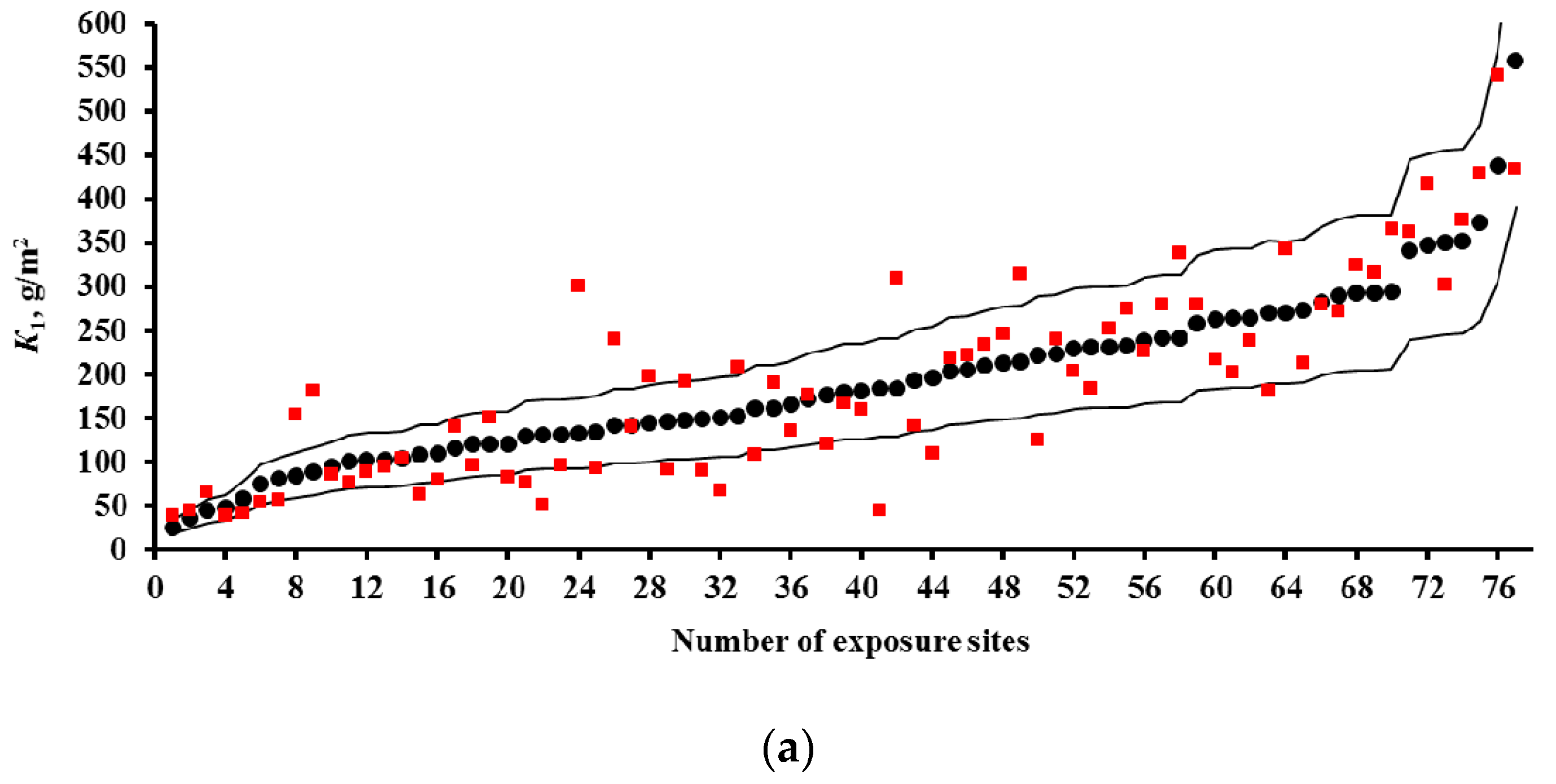
The K = f(SO2) relationships obtained for each program are shown in Figure 1 for steel and in Figure 2 for zinc. In a first approximation, this relationship can be described by the following function for experimental K1 values obtained in a broad range of meteorological atmosphere parameters:
where K1° are the average corrosion losses over the first year (g/m2) in a clean atmosphere for the entire range of T and RH values; and α is the exponent that depends on the metal.
K1 = K1° × [SO2]α,
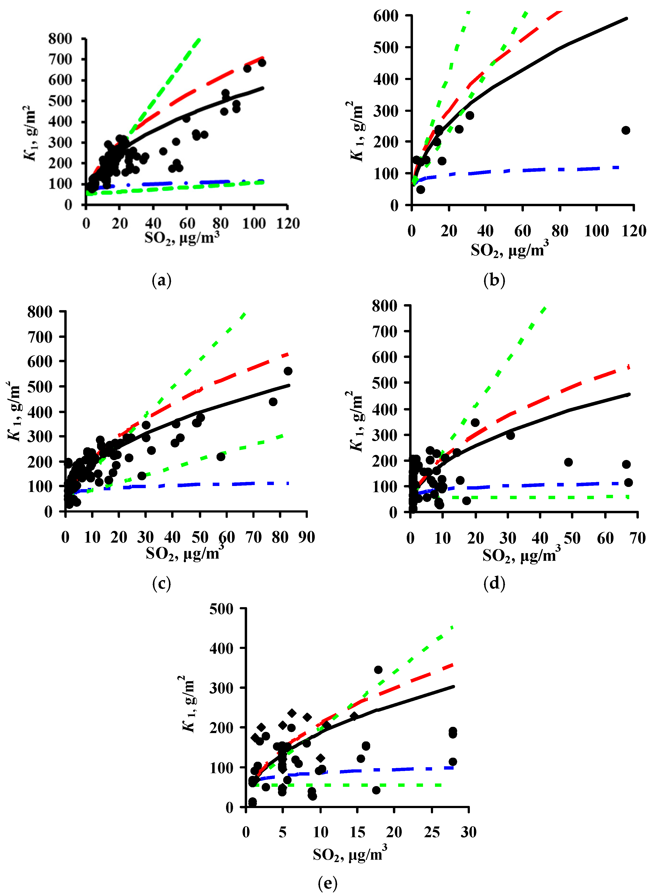
The K1° values corresponding to the mean values of the parameter range of climatic conditions in clean atmospheres were found to be the same for the experimental data of all programs, namely, 63 and 4 g/m2, while α = 0.47 and 0.28 for carbon steel and zinc, respectively. A similar K1° value for carbon steel was also obtained from the Linear DRF, Equation (6). In fact, at background SO2 concentrations = 1 μg/m3 in PE4 test location (Table 3) at TOW = 26 h/year (0.002 of the year), the calculated K1° is to 53 g/m2, while for CO2 test location at TOW = 8760 h/year (entire year) it is 71 g/m2; the mean value is 62 g/m2.
Based on Equation (8), it may be accepted in a first approximation that the effect of [SO2] on corrosion is the same under any climatic conditions and this can be expressed in a DRF by an [SO2]α multiplier, where α = 0.47 or α = 0.28 for steel or zinc, respectively. The K1° values in Equation (8) depend on the climatic conditions and are determined for each test location based on the atmosphere meteorological parameters.
In the development of New DRF, the K1 values were determined using the DRF mathematical formula presented in the Standard DRF and in the Unified DRF, as well as meteorological parameters T, RH, and Prec (Rain for warm climate locations or Prec for cold climate locations). The complex effect of T was taken into account: corrosion losses increase with an increase in T to a certain limit, Tlim; its further increase slows down the corrosion due to radiation heating of the surface of the material and accelerated evaporation of the adsorbed moisture film [12,28]. It has been shown [29] that Tlim is within the range of 9–11 °C. Similarly to Equations (3)–(6), it is accepted that Tlim equals 10 °C. The need to introduce Prec is due to the fact that in northern RF regions, the K1 values are low at high RH, apparently owing not only to low T values but also to the small amount of precipitation, including solid precipitations. The values of the coefficients reflecting the effect of T, RH and Prec on corrosion were determined by regression analysis.
The New DRFs developed for the prediction of K1 (g/m2) for the two temperature ranges have the following forms:
for carbon steel :
and for zinc:
K1 = 7.7 × [SO2]0.47 × exp{0.024 × RH + 0.095 × (T-10) + 0.00056 × Prec} T ≤ 10 °C;
K1 = 7.7 × [SO2]0.47 × exp{0.024 × RH − 0.095 × (T-10) + 0.00056 × Prec} T > 10 °C,
K1 = 7.7 × [SO2]0.47 × exp{0.024 × RH − 0.095 × (T-10) + 0.00056 × Prec} T > 10 °C,
K1 = 0.71 × [SO2]0.28 × exp{0.022 × RH + 0.045 × (T-10) + 0.0001 × Prec} T ≤ 10 °C;
K1 = 0.71 × [SO2]0.28 × exp{0.022 × RH − 0.085 × (T-10) + 0.0001 × Prec} T > 10 °C.
K1 = 0.71 × [SO2]0.28 × exp{0.022 × RH − 0.085 × (T-10) + 0.0001 × Prec} T > 10 °C.
3.2. Predictions of K1 Using Various DRFs for Carbon Steel
Predictions of K1 were performed for all continental test locations with chloride deposition rates ≤2 mg/(m2·day). The results of K1 prediction (K1pr) from Equations (3)–(7), (9), and (10) are presented separately for each test program. To build the plots, the test locations were arranged by increasing experimental K1 values (K1exp). Their sequence numbers are given in Table 2, Table 3 and Table 4. The increase in K1 is caused by an increase in atmosphere corrosivity due to meteorological parameters and SO2 concentration. All the plots are drawn on the same scale. All plots show the lines of prediction errors δ = ±30% (the 1.3 K1exp–0.7 K1exp range). This provides a visual idea of the comparability of K1pr with K1exp for each DRF. The scope of this paper does not include an estimation of the discrepancy between the K1pr values obtained using various DRFs with the K1exp values obtained for each test location under the UN/ECE and RF programs. The scatter of points is inevitable. It results from the imperfection of each DRF and the inaccuracy of experimental data on meteorological parameters, SO2 content, and K1exp values. Let us just note the general regularities of the results on K1pr for each DRF.
The results on K1pr for carbon steel for the UN/ECE program, MICAT project, and RF program are presented in Figure 3, Figure 4 and Figure 5, respectively. It should be noted that according to the Unified DRF (Equation (5)), the K1pr of carbon steel in RF territory [30] had low values. It was also found that the K1pr values are very low for the programs mentioned above. Apparently, the K1pr values (Equation (5)) were calculated in μm rather than in g/m2, as the authors assumed. To convert K1pr in μm to K1pr in g/m2, the 3.54 coefficient in Equation (6) was increased 7.8-fold.
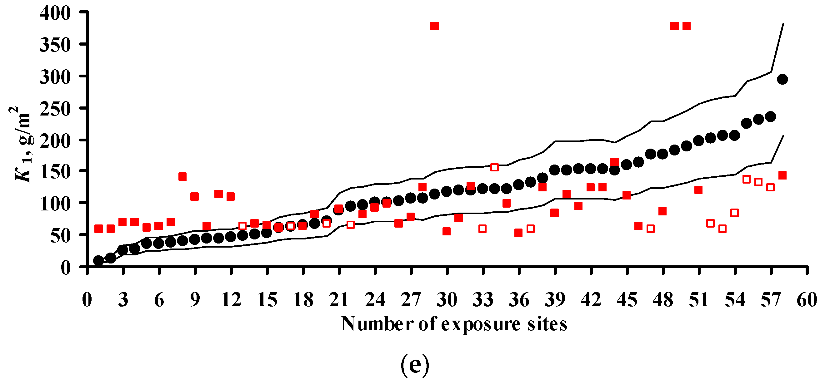
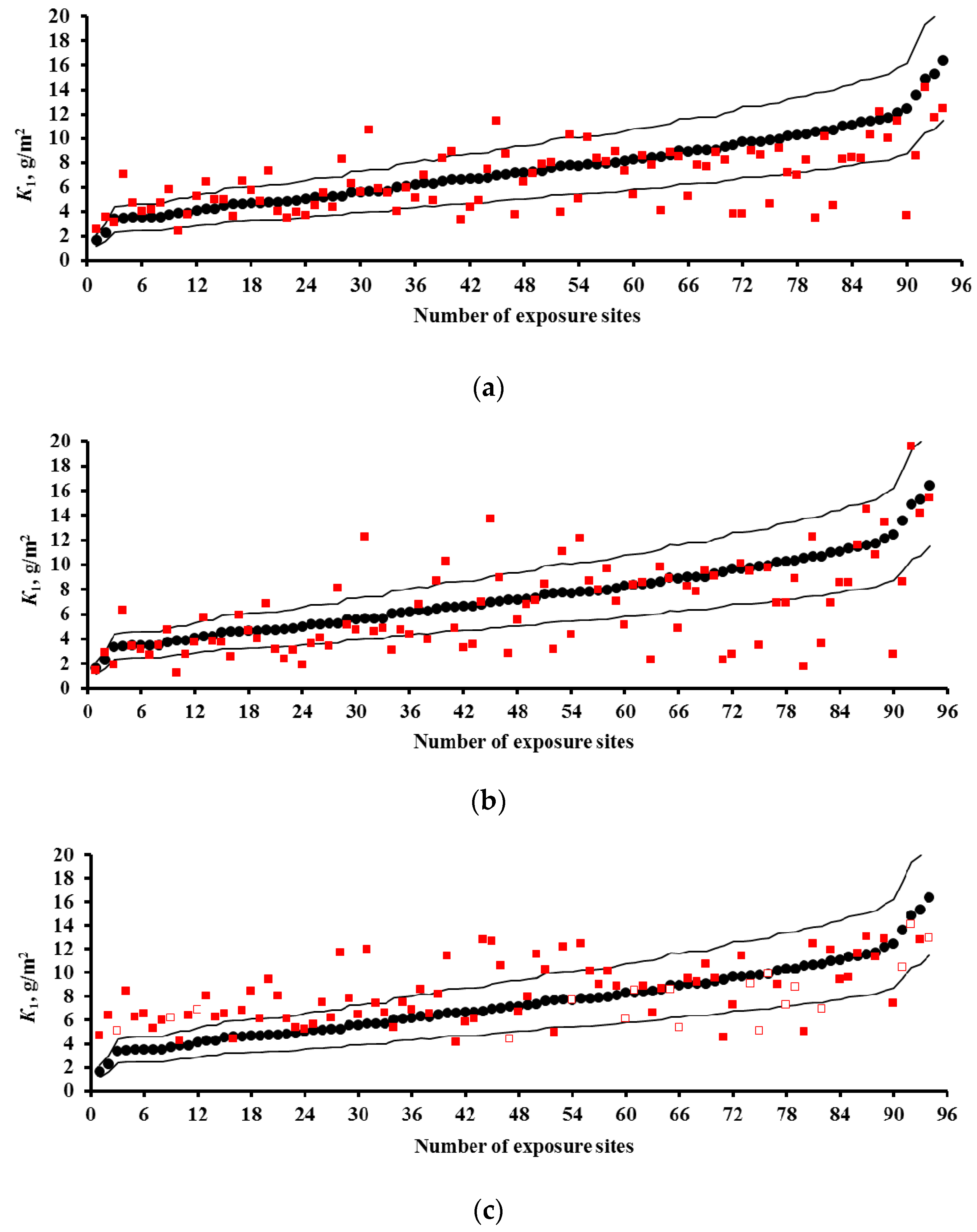
In the UN/ECE program, the K1pr values match K1exp to various degrees; some K1pr values exceed the error δ (Figure 3). Let us describe in general the locations in which K1pr values exceed δ. For the New DRFs (Figure 3a) there are a number of locations with overestimated K1pr and with underestimated K1pr values at different atmosphere corrosivities. For the Standard DRF (Figure 3b) and Linear DRF (Figure 3d), locations with underestimated K1pr values prevail, also at different K1exp. For the Unified DRF (Figure 3c), K1pr are overestimated for locations with small K1exp and underestimated for locations with high K1exp. The possible reasons for such regular differences for K1pr from K1exp will be given based on an analysis of the coefficients in the DRFs.
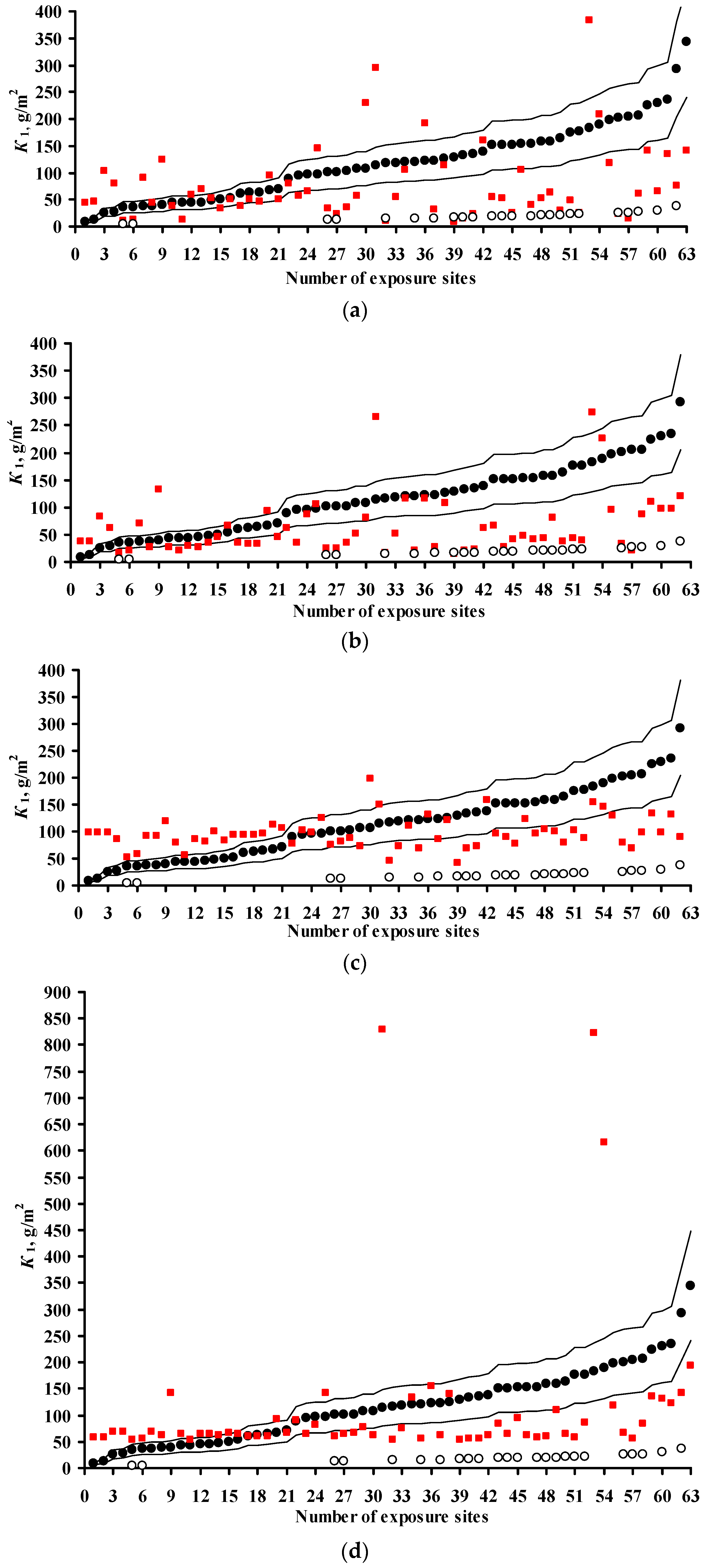
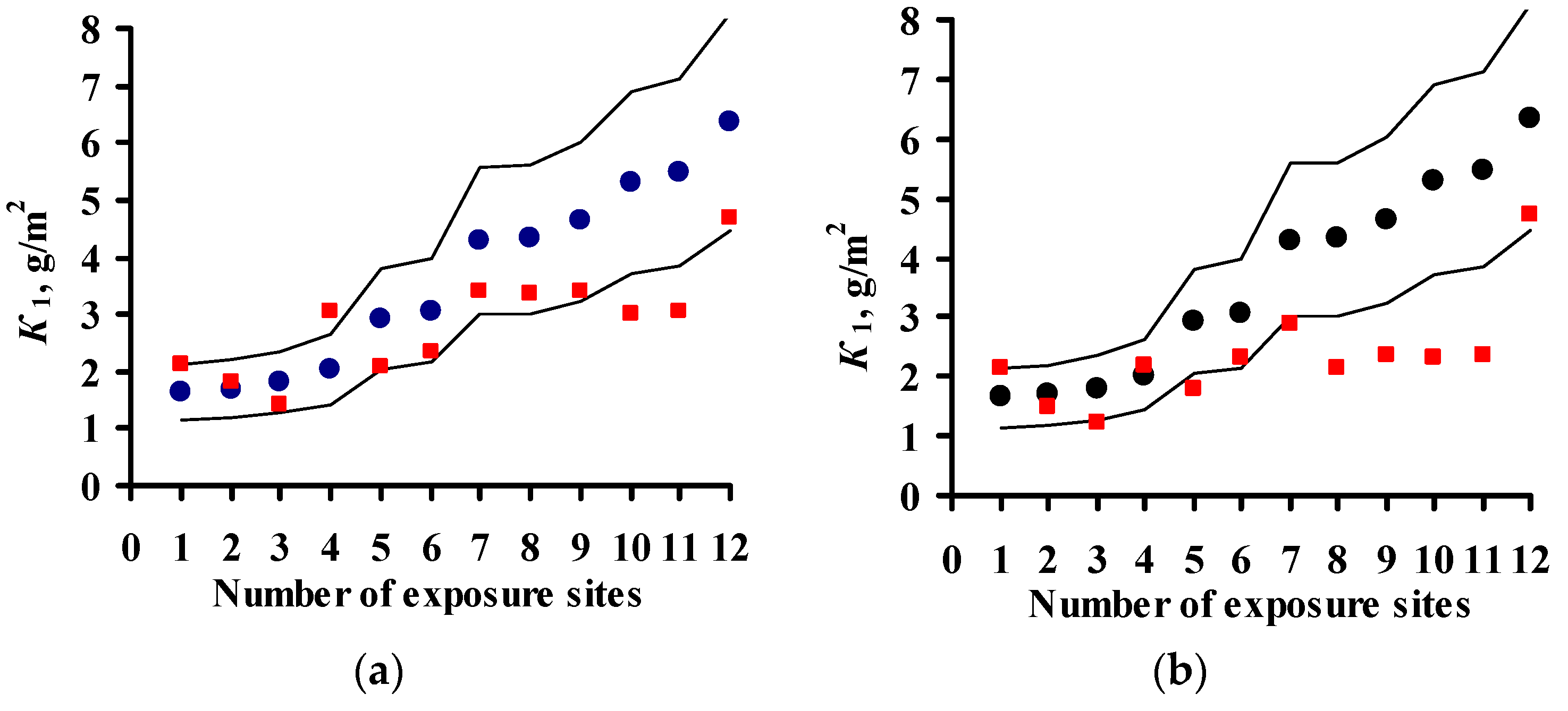
For the MICAT project, K1pr considerably exceeds δ for all DRFs in many locations (Figure 4). Overestimated and considerably overestimated K1pr values are mainly observed in locations with small K1exp, while underestimated K1pr values are mainly observed for locations with high K1exp. Furthermore, for the Linear DRF (Figure 4d), particularly overestimated values are observed in location B6 (No. 31, No. 53, and No. 54) at all exposures. This test location should be noted. The corrosivity parameters under this program reported in [20] are different for some test locations (Table 3). In fact, for B6, the [SO2] value for all exposures is reported to be 28 μg/m3 instead of 67.2; 66.8 and 48.8 μg/m3. Figure 4e presents K1pr for the Linear DRF with consideration for the parameter values reported in [20]. Naturally, K1pr for B6 decreased considerably in comparison with the values in Figure 4d but remained rather overestimated with respect to K1exp.
If all DRFs give underestimated K1pr values for the same locations, this may result from an inaccuracy of experimental data, i.e., corrosivity parameters and/or K1exp values. We did not perform any preliminary screening of the test locations. Therefore, it is reasonable to estimate the reliability of K1exp only in certain locations by comparing them with other locations. Starting from No. 26, K1pr values are mostly either smaller or considerably smaller than K1exp. The locations with underestimated K1pr that are common to all DRFs include: A4 (No. 5, No. 6), B1 (No. 28), B10 (No. 26), B11 (No. 41), E1 (No. 47, No. 48, No. 51), E4 (No. 43, 49, 50), EC1 (No. 45, No. 52, No. 56), CO3 (No. 40, 57), PE4 (No. 32, No. 39), M3 (No. 58, No. 60, No. 62). To perform the analysis, Table 6 was composed. It contains the test locations that, according to our estimates, have either questionable or reliable K1exp values. It clearly demonstrates the unreliability of K1exp in some test locations. For example, in the test locations PE4 and A4, with RH = 33%–51% and TOW = 0.003–0.114 of the year at background [SO2], K1exp are 4.5–16.5 μm (35.1–117 g/m2), while under more corrosive conditions in E8 and M2 with RH = 52%–56% and TOW = 0.100–0.200 of the year and [SO2] = 6.7–9.9 μg/m3, K1exp values are also 3.3–15.2 μm (25.7–118.6 g/m2). The impossibility of high K1 values in PE4 and A4 is also confirmed by the 3D graph of the dependence of K on SO2 and TOW in [20]. Alternatively, for example, in B1, CO3 and B11 with RH = 75%–77% and TOW = 0.172–0.484 of the year and [SO2] = 1–1.7 μg/m3, K1exp = 13.1–26.2 μm (102.2–204.4 g/m2), whereas in A2 and A3 with RH = 72%–76% and TOW = 0.482–0.665 of the year and [SO2] = 1–10 μg/m3, K1exp is as small as 5.6–16.1 μm (43.7–125.6 g/m2). The K1 values reported for locations with uncertain data are 2–4 times higher than the K1 values in trusted locations. The reason for potentially overestimated K1exp values being obtained is unknown. It may be due to non-standard sample treatment or to corrosion-related erosion. It can also be assumed that the researchers (performers) reported K1 in g/m2 rather than in μm. If this assumption is correct, then K1pr values would better match K1exp (Figure 4). Unfortunately, we cannot compare the questionable K1exp values with the K1exp values rejected in the study where an artificial neural network was used [20]. We believe that, of the K1exp values listed, only the data for the test locations up to No. 26 in Figure 4 can be deemed reliable.
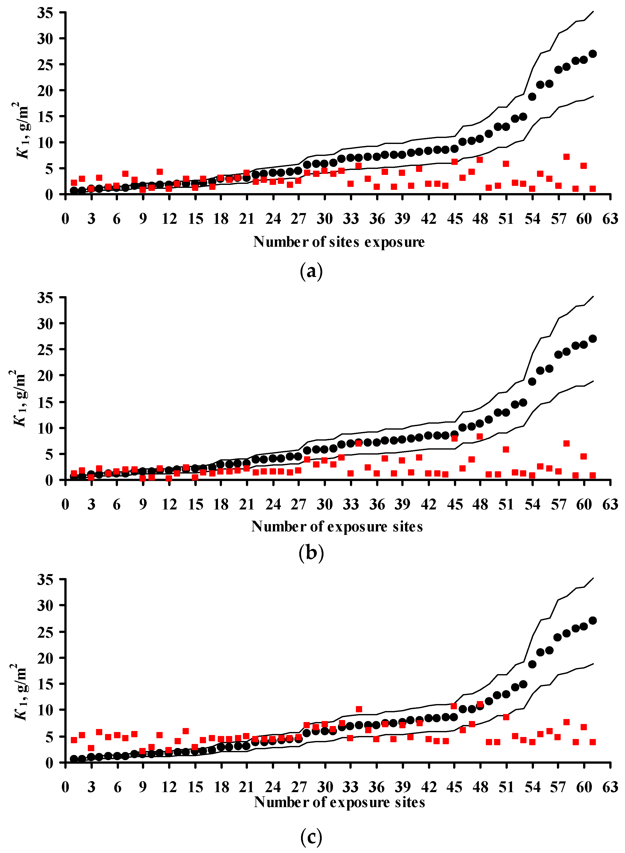
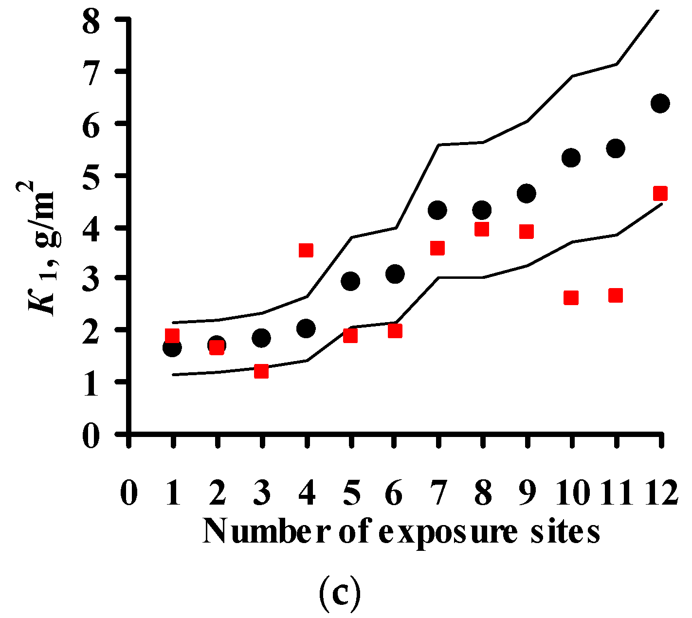
For the RF program, the K1pr values determined by the New DRF and the Standard DRF are pretty comparable with K1exp, but they are considerably higher for the Unified DRF (Figure 5).
The presented figures indicate that all DRFs which have the same parameters but different coefficients predict K1 for same test locations with different degrees of reliability. That is, combinations of various coefficients in DRFs make it possible to obtain K1pr results presented in Figure 3, Figure 4 and Figure 5. In view of this, the analysis of DRFs in order to explain the principal differences of K1pr from K1exp for each DRF appears interesting.
3.3. Analysis of DRFs for Carbon Steel
The DRFs were analyzed by comparison of the coefficients in Equations (3), (5) and (9). Nonlinear DRFs can be represented in the form:
or
where A × ek1·RH × ek2·(T−10) × ek3·Prec = K10.
K1 = A × [SO2]αexp{k1 × RH + k2 × (T−10) + k3 × Prec}
K1 = A × [SO2]α × ek1·RH × ek2·(T−10) × ek3·Prec,
The values of the coefficients used in Equations (3), (5) and (9) are presented in Table 7.
To compare the α values, K1° = 63 g/m2 at [SO2] = 1 μg/m3 was used in Equation (8) for all DRFs. The [SO2]α plots for all the DRFs for all programs are presented in Figure 1. For the New DRF, the line K = f(SO2) was drawn approximately through the mean experimental points from all the test programs. Therefore, one should expect a uniform distribution of error δ, e.g., in Figure 3a. For the Standard DRF, α = 0.52 is somewhat overestimated, which may result in more overestimated K1 values at high [SO2]. However, in Figure 3b for CS1 (No. 76), CS3 (No. 73, 74, 77) and GER10 (No. 76), K1pr overestimation is not observed, apparently due to effects from other coefficients in DRF. For Unified DRF α = 0.13, which corresponds to a small range of changes in K1 as a function of SO2. Therefore, in Figure 3c and Figure 4c, the K1pr present a nearly horizontal band that is raised to the middle of the K1exp range due to a higher value of A = 3.54 μm (27.6 g/m2), Table 7. As a result, the Unified DRF cannot give low K1pr values for rural atmospheres, Figure 3c and Figure 5c, or high K1pr values for industrial atmospheres, Figure 3c.
For the Linear DRF we present K1pr—[SO2] plots for TOW (fraction of a year) within the observed values: 0.043–0.876 for ISO CORRAG program; 0.5–1 based on the data in [19]; 0.17–0.62 from UN/ECE program; 0.003–1 from the MICAT project, and 0.002–0.8 based on the data [20] for the MICAT project, Figure 1. One can see that reliable K1pr are possible in a limited range of TOW and [SO2]. The K1pr values are strongly overestimated at high values of these parameters (Figure 4c,d). That is, the Linear model has a limited applicability at combinations of TOW and [SO2] that occur under natural conditions. Furthermore, according to the Linear DRF, the range of K1pr in clean atmosphere is 53–71 g/m2, therefore the K1pr values in clean atmosphere lower than 53 g/m2 (Figure 3d and Figure 4d,e) or above 71 g/m2 cannot be obtained. Higher K1pr values can only be obtained due to [SO2] contribution. The underestimated K1pr values in comparison with K1exp for the majority of test locations (Figure 3d) are apparently caused by the fact that the effects of other parameters, e.g., T, on corrosion are not taken into account.
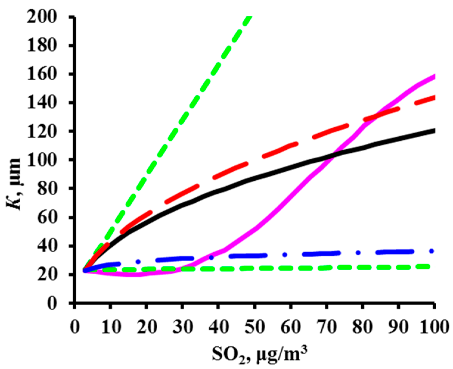
Figure 6 compares K = f(SO2) for all the models with the graphical representation of the dependence reported in [20] (for [SO2], mg/(m2·d) values were converted to μg/m3). The dependence in [20] is presented for a constant temperature, whereas the dependences given by DRFs are given for average values in the entire range of meteorological parameters in the test locations. Nevertheless, the comparison is of interest. Below 70 and 80 μg/m3, according to [20], K has lower values than those determined by the New DRF and Standard DRF, respectively, while above these values, K has higher values. According to the Unified DRF, K has extremely low values at all [SO2] values, whereas according to the Linear DRF (TOW from 0.03 to 1), the values at TOW = 1 are extremely high even at small [SO2].
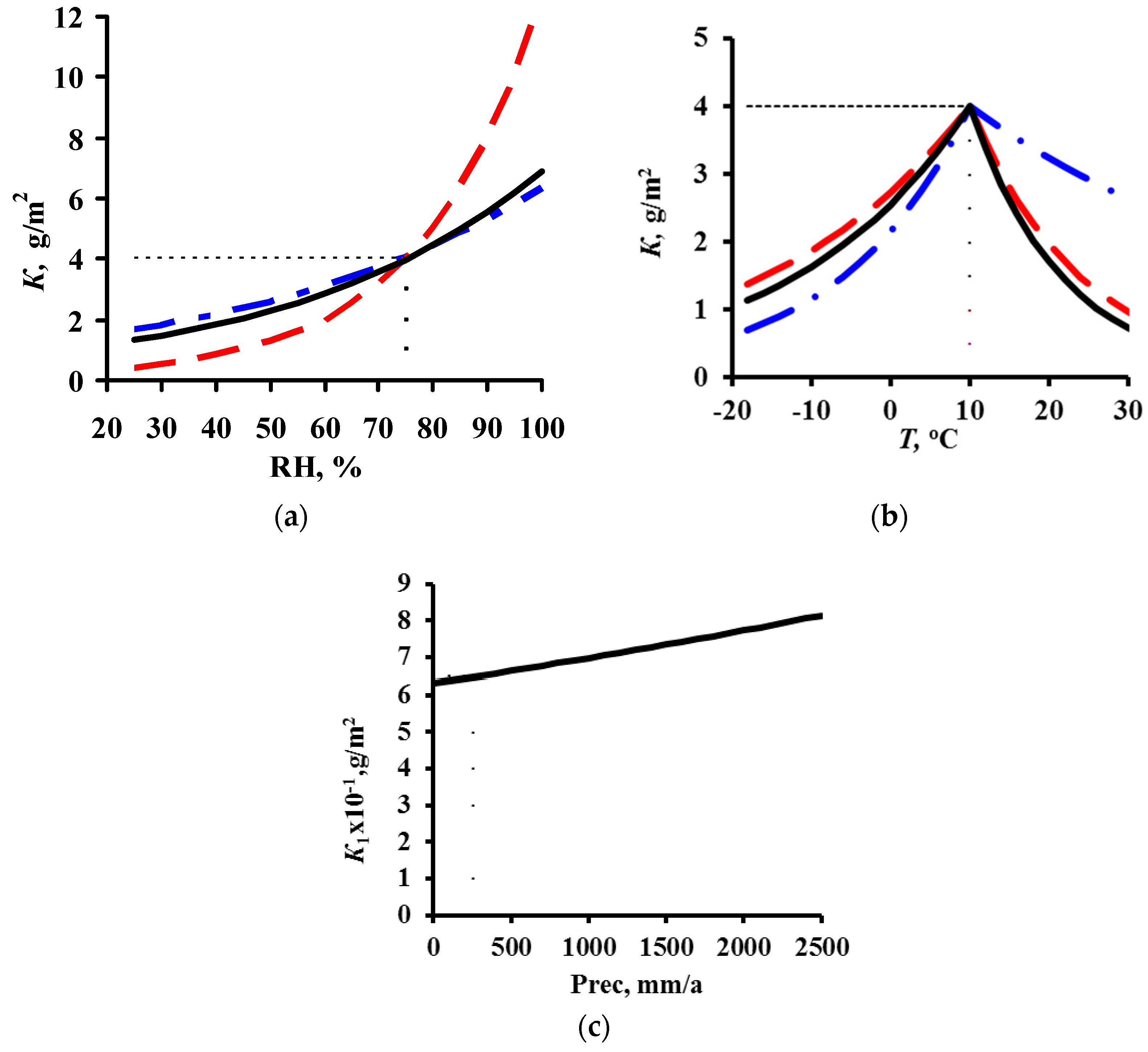
To perform a comparative estimate of k1 and k2, let us use the value Tlim = 10 °C accepted in the DRF, i.e., where the temperature dependence changes. Furthermore, it is necessary to know the K1 value in clean atmosphere at Tlim and at the RH that is most common at this temperature. These data are unknown at the moment. Therefore, we’ll assume that at Tlim = 10 °C and RH = 75%, K = 63 g/m2. The dependences of K on T and RH under these conditions and with consideration for the corresponding k1 and k2 for each DRF are presented in Figure 7.
The nearly coinciding k1 values (0.020 for the Unified DRF and Standard DRF, and 0.024 for the New DRF, Table 8) result in an insignificant difference in the RH effect on K (Figure 7a).
The temperature coefficient k2 has a considerable effect on K. For the Unified DRF, the k2 values of 0.059 (−0.036) for T ≤ 10 °C (T > 10 °C) create the lowest decrease in K with a T decrease (increase) in comparison with the other DRFs (Figure 7b). A consequence of such k2 values can be demonstrated by examples. Due to the temperature effect alone, K ~ 15 g/m2 at T = −12 °C (Figure 7b) and K~45 g/m2 at T = 20 °C. The effects of other parameters and account for the A value would result in even more strongly overestimated Kpr values. For comparison: in Bilibino at T = −12.2 °C and RH = 80%, K1exp = 5.4 g/m2 (Table 4) and Kpr = 42 g/m2 (Figure 5). In A3 test location, at T = 20.6 °C and RH = 76%, K1exp = 44.5 g/m2 (Table 4), while due to A and other parameters, K1pr = 86.2 g/m2, Figure 4c.
In the Standard DRF, the k2 values are higher than in the Unified DRF: 0.150 and −0.054 for T ≤ 10 °C and T > 10 °C, respectively, so a greater K decrease is observed, especially at T ≤ 10 °C, Figure 7b. At low T, the K values are small, e.g., K ~ 2 g/m2 at T = −12 °C. In K1pr calculations, the small K are made higher due to A, and they are higher in polluted atmospheres due to higher α = 0.52. As a result, Kpr are quite comparable with Kexp, Figure 3b. However, let us note that Kpr is considerably lower than Kexp in many places. Perhaps, this is due to an abrupt decrease in K in the range T ≤ 10 °C. This temperature range is mostly met in test locations under the UN/ECE program.
In the New DRF, k2 has an intermediate value at T ≤ 10 °C and the lowest value at T > 10 °C, whereas A has the lowest value. It is more difficult to estimate the k2 value with similar k2 values in the other DRFs, since the New DRF uses one more member, i.e., ek3·Prec. The dependence of K on Prec is presented in Figure 7c. The following arbitrary values were used to demonstrate the possible effect of Prec on K: K = 7.8 g/m2 at Prec = 632 mm/year. For example, in location PE5 (UN/ECE program) with Prec = 632 mm/year, K = 7.8 g/m2 at T = 12.2 °C and RH = 67%. The maximum Prec was taken as 2500 mm/year, e.g., it is 2144 mm/year in NOR23 (UN/ECE program) and 2395 mm/year in B8 (MICAT project). It follows from the figure that, other conditions being equal, K can increase from 5.4 to 22.6 g/m2 just due to an increase in Prec from 0 to 2500 mm/year at k3 = 0.00056 (Table 7).
Thus, it has been shown that the coefficients for each parameter used in the DRFs vary in rather a wide range. The most reliable K1pr can be reached if, in order to find the most suitable coefficients, the DRFs are based on the K = f(SO2) relationship obtained.
3.4. Predictions of K1 Using Various DRFs for Zinc
The results on K1pr for zinc for the UN/ECE program, MICAT project, and RF program are presented in Figure 8, Figure 9 and Figure 10, respectively. In the UN/ECE program, the differences between the K1pr and K1exp values for zinc are more considerable than those for carbon steel. This may be due not only to the imperfection of the DRFs and the inaccuracy of the parameters and K1exp, but also to factors unaccounted for in DRFs that affect zinc. For all the DRFs, the K1pr values match K1exp to various extent; some of the latter exceed the error δ (±30%). Let us estimate the discrepancy between K1pr and K1exp for those K1pr that exceed δ. For the New DRF (Figure 8a) and the Standard DRF (Figure 8b), overestimated K1pr values are observed for low and medium K1exp, while underestimated ones are observed for medium and high K1exp. In general, the deviations of K1pr from K1exp are symmetrical for these DRFs, but the scatter of K1pr is greater for the Standard DRF. For Unified DRF (Figure 8c), K1pr are mostly overestimated, considering that the ∆K[H+] = 0.029Rain[H+] component was not taken into account for some test locations due to the lack of data on [H+]. The ∆K[H+] value can be significant, e.g., 2.35 g/m2 in US39 or 5.13 g/m2 in CS2.
With regard to the MICAT project, the New and Unified DRFs (Figure 9a,c) give overestimated K1pr at low K1exp, but the Standard DRF gives K1pr values comparable to K1exp (Figure 9b). Starting from test locations No. 33–No. 36, the K1pr values for all the DRFs are underestimated or significantly underestimated. It is evident from Figure 2b that rather many test locations with small [SO2] have extremely high K1exp. This fact confirms the uncertainty of experimental data from these locations, as shown for carbon steel as well. The following test locations can be attributed to this category: A3 (No. 43, No. 44, No. 53), B10 (No. 50), B11 (No. 49), B12 (No. 57), CO2 (No. 55, No. 58, No. 60), CO3 (No. 54, No. 61), PE6 (No. 36, No. 38), and M3 (No. 35, No. 59). There is little sense in making K1 predictions for these locations.
For the RF program, the K1pr values calculated by the New and Unified DRFs are more comparable to K1exp than those determined using the Standard DRF (Figure 10).
3.5. Analysis of DRFs for Zinc
As for steel, DRFs were analyzed by comparison of their coefficients. The nonlinear DRFs for zinc can be represented in the form:
or
K1 = A × [SO2]α× exp{k1 × RH + k2 × (T−10) + k3 × Prec}+ B × Rain × [H+]
K1 = A × [SO2]α × ek1·RH × ek2·(T−10) × ek3·Prec + B × Rain × [H+].
The values of the coefficients used in Equations (4), (6) and (10) are presented in Table 8.
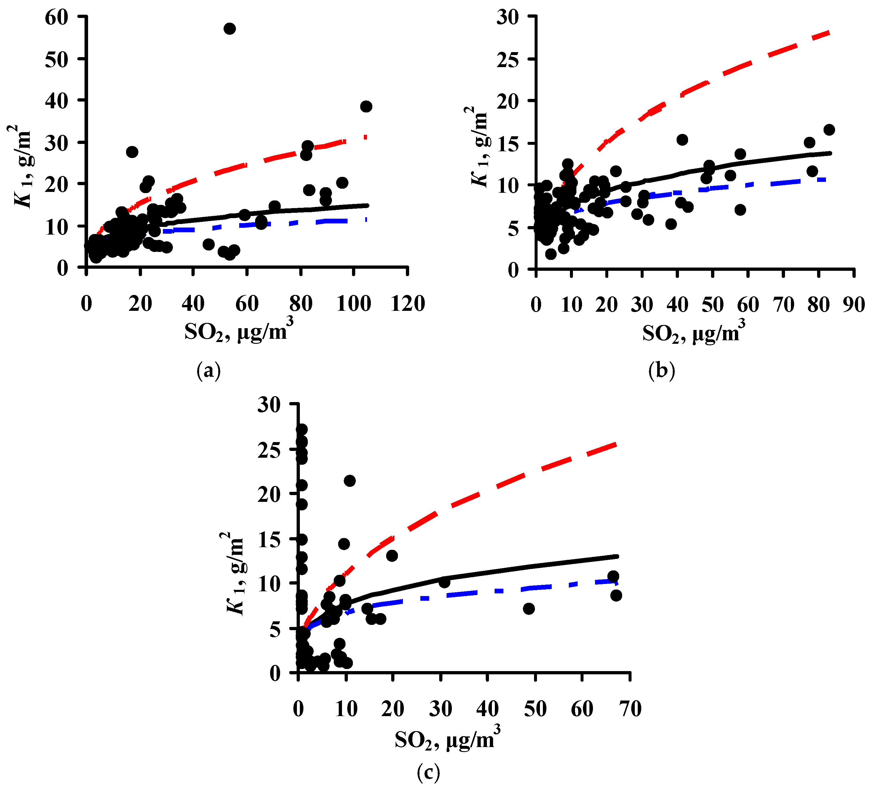
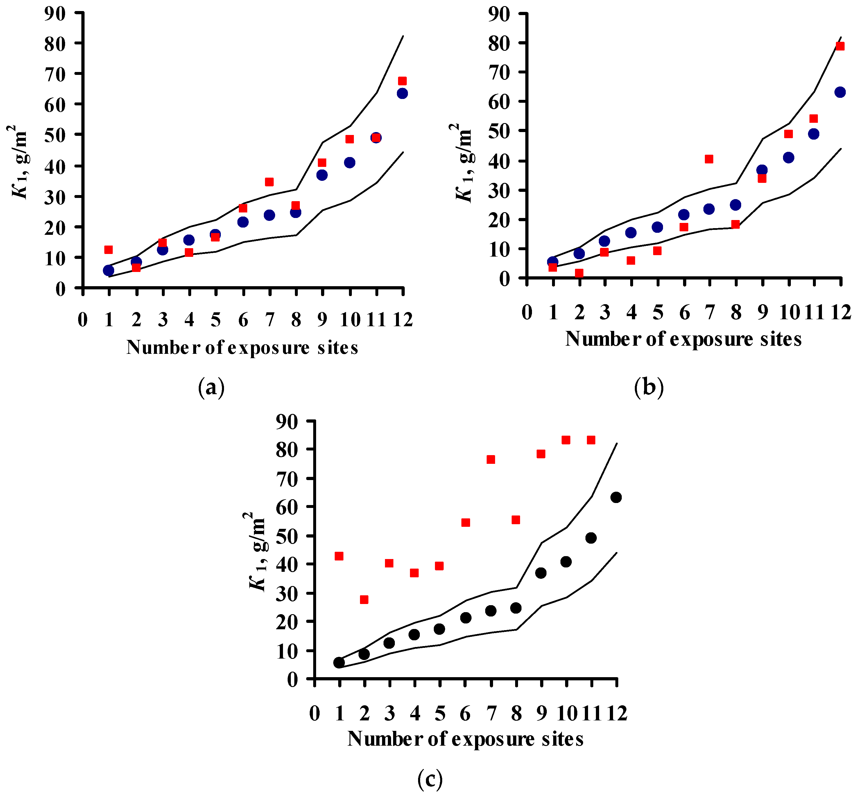
To compare the α values, K1 = 4 g/m2 at [SO2] = 1 μg/m3 was used for all DRFs. Let us note that the value K1 = 4 g/m2 was obtained during the estimation of K = f(SO2) for the development of the New DRF. The plots for all the programs are presented in Figure 2. For the New DRF, the line at α = 0.28 mostly passes through the average experimental points. For the Standard DRF, α = 0.44 is overestimated considerably, which may result in overestimated K1pr, especially at high [SO2]. For the Unified DRF at α = 0.22, the line passes, on average, slightly below the experimental points. The low α value, as for carbon steel, does not give a wide range of K values as a function of [SO2], which may result in underestimated K1pr, especially at high [SO2].
Let us assume for a comparative estimate of k1 and k2 that K = 4 g/m2 in a clean atmosphere at Tlim = 10 °C and RH = 75%. Figure 11 demonstrates the plots of K versus these parameters under these starting conditions. The Standard DRF (k1 = 0.46) shows an abrupt variation in K vs. RH. According to this relationship, at the same temperature, the K value should be 0.5 g/m2 at RH = 30% and 12.6 g/m2 at RH = 100%. According to the New DRF and Unified DRF with k1 = 0.22 and 0.18, respectively, the effect of RH is weaker, therefore K = 1.5 and 1.8 g/m2 at RH = 30%, respectively, and K = 6.9 and 6.4 g/m2 at RH = 100%, respectively.
The effect of temperature on K is shown in Figure 11b. In the New DRF, k2 = 0.045 at T ≤ 10 °C has an intermediate value; at T > 10 °C, k2 = −0.085 has the largest absolute value, which corresponds to an abrupt decrease in K with an increase in temperature. In the Unified DRF, k2 = −0.021 at T > 10 °C, i.e., an increase in temperature results in a slight decrease in K. As for the effect of A, this also contributes to higher K1pr values despite the small α value.
In the Standard DRF, the value A = 0.0929 (g/m2), which is ~8 times smaller than in the New DRF, and a small k2 = −0.71 at T > 10 °C were taken to compensate the K1pr overestimation due to the combination of high values, α = 0.44 and k1 = 0.46. In the Unified DRF, the high A value that is ~2 times higher than in the New DRF is not compensated by the combination of the low values, α = 0.22 and k2 = −0.021 at T > 10 °C. Therefore, the K1pr values are mostly overestimated, Figure 8c and Figure 9c for trusted test locations. However, small K1pr values were attained for low T at k2 = 0.62, Figure 10c.
The effect of Prec on K at k3 = 0.0001, which is taken into account only in the New DRF, given under the assumption that K = 0.65 in a clean atmosphere at Prec (Rain) = 250 mm/year, T = 15 °C and RH = 60% (e.g., location E5 in the MICAT project), is shown in Figure 11c. Upon an increase in Prec (Rain) from 250 to 2500 mm/year, K can increase from 0.65 to 0.81 g/m2.
As for carbon steel, the above analysis of coefficients in the DRFs for zinc confirms that the coefficients can be varied to obtain reliable K1pr values. The New DRF based on K = f(SO2) gives the most reliable K1pr values for zinc.
4. Estimation of Coefficients in DRFs for Carbon Steel and Zinc
Let us first note that the starting conditions that we took to demonstrate the effect of various atmosphere corrosivity parameters on K of carbon steel and zinc (Figure 7 and Figure 11) may not match the real values. However, the plots obtained give an idea on K variations depending on the coefficients in the DRFs.
For continental test locations under all programs, the K1exp values are within the following ranges: for carbon steel, from 6.3 (Oimyakon, RF program) to 577 g/m2 (CS3, UN/ECE program); for zinc, from 0.65 (E5, MICAT project) to 16.41 g/m2 (CS3, UN/ECE program). That is, the difference in the corrosion losses is at least ~10–35 fold, the specific densities of these metals being nearly equal. Higher K1pr values for steel than for zinc are attained using different coefficients at the parameters in the DRFs.
In the New DRFs, A is 7.7 and 0.71 g/m2 for carbon steel and zinc, respectively, i.e., the difference is ~10-fold. Higher K1pr values for steel than for zinc were obtained chiefly due to the contribution of [SO2]α at α = 0.47 and 0.28, respectively. The values of RH and Prec affect the corrosion of steel more strongly than they affect zinc corrosion. The coefficients for these parameters are: k1 = 0.024 and 0.022; k3 = 0.00056 and 0.0001 for steel and zinc, respectively. However, the temperature coefficients (k2 = 0.095 and −0.095 for steel; k2 = 0.045 and −0.085 for zinc) indicate that, with a deviation of T from 10 °C, the corrosion process on steel is hindered to a greater extent than on zinc.
In the Standard DRF, A is 1.77 and 0.0129 μm for carbon steel and zinc, respectively, i.e., the difference is ~137-fold. The α value for steel is somewhat higher than that for zinc, i.e., 0.52 and 0.44 respectively, which increases the difference of K1pr for steel from that for zinc. As shown above, the difference should not be greater than 35-fold. This difference is compensated by the 2.3-fold higher effect of RH on zinc corrosion than on steel corrosion (k1 = 0.046 and 0.020 for zinc and steel, respectively). Furthermore, the temperature coefficient k2 at T ≤ 10 °C for steel is 3.95 times higher than that for zinc. This indicates that steel corrosion slows down abruptly in comparison with zinc as T decreases below 10 °C. At T > 10 °C, the k2 values for steel and zinc are comparable. Taking the values of the coefficients presented into account, the K1pr values for steel are 15-fold higher, on average, than those for zinc at T ≤ 10 °C, but ~60-fold at T > 10 °C. Of course, this is an approximate estimate of the coefficients used in the Standard DRF.
In the Unified DRF, A is 3.54 and 0.188 μm for carbon steel and zinc, respectively, i.e., the difference is ~19-fold. The α value for steel is lower than that for zinc, i.e., 0.13 and 0.22 respectively, which decreases the difference of K1pr of steel from that of zinc. Conversely, the RH value affects steel corrosion somewhat more strongly than that of zinc (k1 = 0.020 and 0.018 for steel and zinc, respectively). The k2 values for steel and zinc are comparable in both temperature ranges. The ∆K[H+] component was introduced only for zinc, which somewhat complicates the comparison of the coefficients in these DRFs.
All the presented DRFs are imperfect not only because of the possible inaccuracy of the mathematical expressions as such, but also due to the inaccuracy of the coefficients used in the DRFs. The K1pr values obtained using the New DRF match K1exp most accurately. However, while the α values that were assumed to be 0.47 and 0.28 for carbon steel and zinc, respectively, may be considered as accurate in a first approximation, the other coefficients need to be determined more accurately by studying the effect of each atmosphere corrosivity parameter on corrosion, with the other parameters being unchanged. Studies of this kind would allow each coefficient to be estimated and DRFs for reliable prediction of K1 in atmospheres with various corrosivity to be created.
5. Conclusions
- K = f(SO2) plots of corrosion losses of carbon steel and zinc vs. sulfur dioxide concentration were obtained to match, to a first approximation, the mean meteorological parameters of atmosphere corrosivity.
- Based on the K = f(SO2) relationships obtained, with consideration for the nonlinear effect of temperature on corrosion, New DRFs for carbon steel and zinc in continental territories were developed.
- Based on the corrosivity parameters at test locations under the UN /ECE and RF programs and the MICAT project, predictions of first-year corrosion losses of carbon steel and zinc were given using the New DRF, Standard DRF, and Unified DRF, as well as the linear model for carbon steel obtained in [20] with the aid of an artificial neural network. The predicted corrosion losses are compared with the experimental data for each DRF. It was shown that the predictions provided by the New DRFs for the first-year match the experimental data most accurately.
- An analysis of the values of the coefficients used in the DRFs for the prediction of corrosion losses of carbon steel and zinc is presented. It is shown that more accurate DRFs can be developed based on quantitative estimations of the effects of each atmosphere corrosivity parameter on corrosion.
Acknowledgments
We are grateful to Manuel Morcillo for valuable comments.
Author Contributions
Y.M.P. performed the modelling and analysis and wrote the paper. A.I.M. contributed the discussion of the data.
Conflicts of Interest
The authors declare no conflict of interest.
References
- McCuen, R.H.; Albrecht, P.; Cheng, J.G. A New Approach to Power-Model Regression of Corrosion Penetration Data. In Corrosion Forms and Control for Infrastructure; Chaker, V., Ed.; American Society for Testing and Materials: Philadelphia, PA, USA, 1992. [Google Scholar]
- Syed, S. Atmospheric corrosion of materials. Emir. J. Eng. Res. 2006, 11, 1–24. [Google Scholar]
- De la Fuente, D.; Castano, J.G.; Morcillo, M. Long-term atmospheric corrosion of zinc. Corros. Sci. 2007, 49, 1420–1436. [Google Scholar] [CrossRef]
- Landolfo, R.; Cascini, L.; Portioli, F. Modeling of metal structure corrosion damage: A state of the art report. Sustainability 2010, 2, 2163–2175. [Google Scholar] [CrossRef]
- Morcillo, M.; de la Fuente, D.; Diaz, I.; Cano, H. Atmospheric corrosion of mild steel (article review). Rev. Metal. 2011, 47, 426–444. [Google Scholar] [CrossRef]
- De la Fuente, D.; Diaz, I.; Simancas, J.; Chico, B.; Morcillo, M. Long-term atmospheric corrosion of mild steel. Corros. Sci. 2011, 53, 604–617. [Google Scholar] [CrossRef]
- Morcillo, M.; Chico, B.; Diaz, I.; Cano, H.; de la Fuente, D. Atmospheric corrosion data of weathering steels: A review. Corros. Sci. 2013, 77, 6–24. [Google Scholar] [CrossRef]
- Surnam, B.Y.R.; Chiu, C.W.; Xiao, H.P.; Liang, H. Long term atmospheric corrosion in Mauritius. CEST 2015, 50, 155–159. [Google Scholar] [CrossRef]
- Panchenko, Y.M.; Marshakov, A.I. Long-term prediction of metal corrosion losses in atmosphere using a power-linear function. Corros. Sci. 2016, 109, 217–229. [Google Scholar] [CrossRef]
- Corrosion of Metals and Alloys—Corrosivity of Atmospheres—Guiding Values for the Corrosivity Categories; ISO 9224:2012(E); International Standards Organization: Geneva, Switzerlands, 2012.
- Rosales, B.M.; Almeida, M.E.M.; Morcillo, M.; Uruchurtu, J.; Marrocos, M. Corrosion y Proteccion de Metales en las Atmosferas de Iberoamerica; Programma CYTED: Madrid, Spain, 1998; pp. 629–660. [Google Scholar]
- Tidblad, J.; Kucera, V.; Mikhailov, A.A. Statistical Analysis of 8 Year Materials Exposure and Acceptable Deterioration and Pollution Levels; UN/ECE ICP on Effects on Materials; Swedish Corrosion Institute: Stockholm, Sweden, 1998; p. 49. [Google Scholar]
- Tidblad, J.; Mikhailov, A.A.; Kucera, V. Unified Dose-Response Functions after 8 Years of Exposure. In Quantification of Effects of Air Pollutants on Materials; UN ECE Workshop Proceedings; Umweltbundesamt: Berlin, Germany, 1999; pp. 77–86. [Google Scholar]
- Tidblad, J.; Kucera, V.; Mikhailov, A.A.; Henriksen, J.; Kreislova, K.; Yaites, T.; Stöckle, B.; Schreiner, M. UN ECE ICP Materials. Dose-response functions on dry and wet acid deposition effects after 8 years of exposure. Water Air Soil Pollut. 2001, 130, 1457–1462. [Google Scholar] [CrossRef]
- Tidblad, J.; Mikhailov, A.A.; Kucera, V. Acid Deposition Effects on Materials in Subtropical and Tropical Climates. Data Compilation and Temperate Climate Comparison; KI Report 2000:8E; Swedish Corrosion Institute: Stockholm, Sweden, 2000; pp. 1–34. [Google Scholar]
- Tidblad, J.; Mikhailov, A.A.; Kucera, V. Application of a Model for Prediction of Atmospheric Corrosion for Tropical Environments. In Marine Corrosion in Tropical Environments; Dean, S.W., Delgadillo, G.H., Bushman, J.B., Eds.; American Society for Testing and Materials: West Conshohocken, PA, USA, 2000; p. 18. [Google Scholar]
- Tidblad, J.; Kucera, V.; Mikhailov, A.A.; Knotkova, D. Improvement of the ISO Classification System Based on Dose-Response Functions Describing the Corrosivity of Outdoor Atmospheres. In Outdoor Atmospheric Corrosion, ASTM STP 1421; Townsend, H.E., Ed.; American Society for Testing and Materials: West Conshohocken, PA, USA, 2002; p. 73. [Google Scholar]
- Corrosion of Metals and Alloys—Corrosivity of Atmospheres—Classification, Determination and Estimation; ISO 9223:2012(E); International Standards Organization: Geneva, Switzerlands, 2012.
- Cai, J.; Cottis, R.A.; Lyon, S.B. Phenomenological modelling of atmospheric corrosion using an artificial neural network. Corros. Sci. 1999, 41, 2001–2030. [Google Scholar] [CrossRef]
- Pintos, S.; Queipo, N.V.; de Rincon, O.T.; Rincon, A.; Morcillo, M. Artificial neural network modeling of atmospheric corrosion in the MICAT project. Corros. Sci. 2000, 42, 35–52. [Google Scholar] [CrossRef]
- Diaz, V.; Lopez, C. Discovering key meteorological variables in atmospheric corrosion through an artificial neural network model. Corros. Sci. 2007, 49, 949–962. [Google Scholar] [CrossRef]
- Kenny, E.D.; Paredes, R.S.C.; de Lacerda, L.A.; Sica, Y.C.; de Souza, G.P.; Lazaris, J. Artificial neural network corrosion modeling for metals in an equatorial climate. Corros. Sci. 2009, 51, 2266–2278. [Google Scholar] [CrossRef]
- Reddy, N.S. Neural Networks Model for Predicting Corrosion Depth in Steels. Indian J. Adv. Chem. Sci. 2014, 2, 204–207. [Google Scholar]
- Knotkova, D.; Kreislova, K.; Dean, S.W. ISOCORRAG International Atmospheric Exposure Program: Summary of Results; ASTM Series 71; ASTM International: West Conshohocken, PA, USA, 2010. [Google Scholar]
- Morcillo, M. Atmospheric corrosion in Ibero-America. The MICAT project. In Atmospheric Corrosion; Kirk, W.W., Lawson, H.H., Eds.; ASTM STP 1239; American Society for Testing and Materials: Philadelphia, PA, USA, 1995; pp. 257–275. [Google Scholar]
- Panchenko, Y.M.; Shuvakhina, L.N.; Mikhailovsky, Y.N. Atmospheric corrosion of metals in Far Eastern regions. Zashchita Metallov 1982, 18, 575–582. (In Russian) [Google Scholar]
- Knotkova, D.; Vlckova, J.; Honzak, J. Atmospheric Corrosion of Weathering Steels. In Atmospheric Corrosion of Metals; Dean, S.W., Jr., Rhea, E.C., Eds.; ASTM STP 767; American Society for Testing and Materials: Philadelphia, PA, USA, 1982; pp. 7–44. [Google Scholar]
- Tidblad, J.; Mikhailov, A.A.; Kucera, V. Model for the prediction of the time of wetness from average annual data on relative air humidity and air temperature. Prot. Met. 2000, 36, 533–540. [Google Scholar] [CrossRef]
- Feliu, S.; Morcillo, M.; Feliu, J.S. The prediction of atmospheric corrosion from meteorological and pollution parameters. I. Annual corrosion. Corros. Sci. 1993, 34, 403–422. [Google Scholar] [CrossRef]
- Panchenko, Y.M.; Marshakov, A.I.; Nikolaeva, L.A.; Kovtanyuk, V.V.; Igonin, T.N.; Andryushchenko, T.A. Comparative estimation of long-term predictions of corrosion losses for carbon steel and zinc using various models for the Russian territory. CEST 2017, 52, 149–157. [Google Scholar] [CrossRef]
Figure 1.
Dependence of first-year corrosion losses of steel (K1) on SO2 concentration based on data from ISO CORRAG program (a), Ref. [19] (b), UN/ECE program (c), MICAT project (d), and data from MICAT project cited in [20] (e). ▬▬—α = 0.47 (New DRF), ▬ ▬—α = 0.52 (Standard DRF), ▬●▬—α = 0.13 (Unified DRF), ─ ─ ─—model [20] for TOW ranges in accordance with the data in Table 2, Table 3, Table 4 and Table 5.

Figure 2.
Dependence of first-year corrosion losses of zinc (K1) on SO2 concentration based on the data from ISO CORRAG program (a), UN/ECE program (b), and MICAT project (c). ▬▬—α = 0.28 (New DRF), ▬ ▬—α = 0.44 (Standard DRF), ▬●▬—α = 0.22 (Unified DRF).
Figure 2.
Dependence of first-year corrosion losses of zinc (K1) on SO2 concentration based on the data from ISO CORRAG program (a), UN/ECE program (b), and MICAT project (c). ▬▬—α = 0.28 (New DRF), ▬ ▬—α = 0.44 (Standard DRF), ▬●▬—α = 0.22 (Unified DRF).

Figure 3.
Carbon steel. UN/ECE program. K1 predictions by the New DRF (a); Standard DRF (b); Unified DRF (c); and Linear DRF [20] (d). ●—experimental K1 data; ■—K1 predictions. Thin lines show the calculation error (± 30%). The numbers of the exposure sites are given in accordance with Table 2.

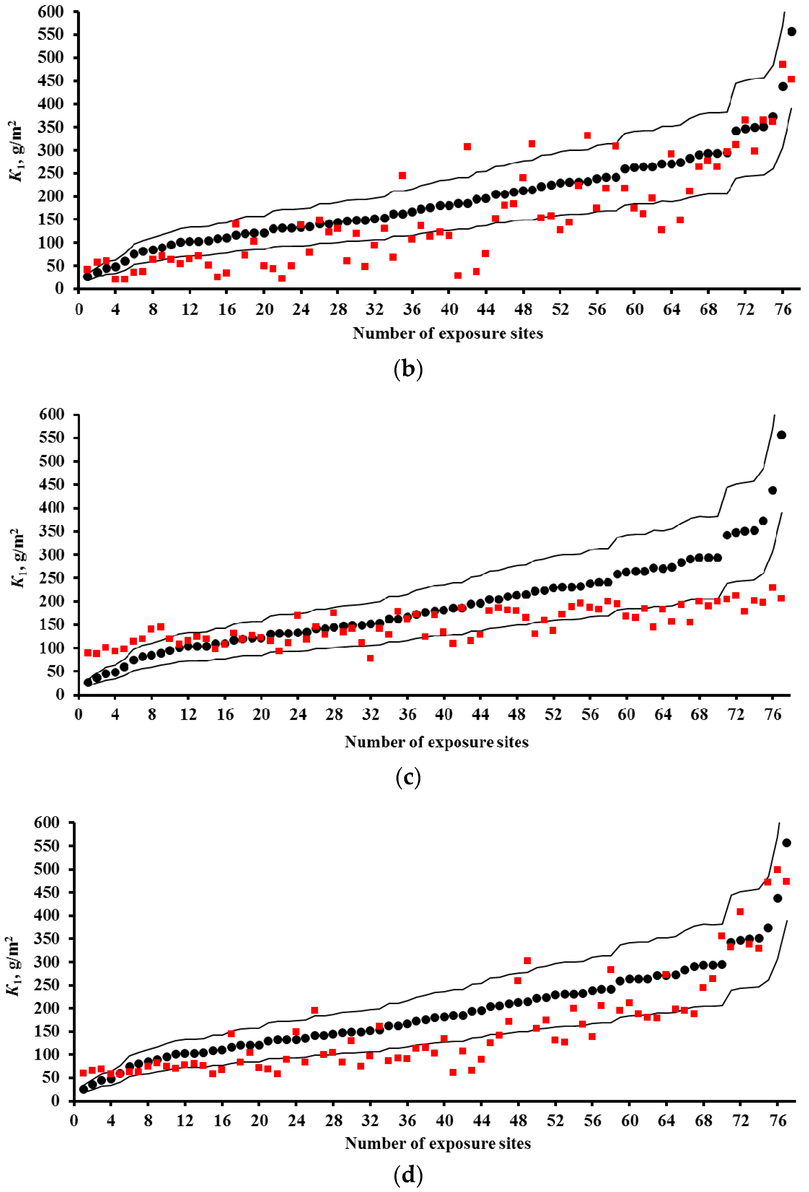
Figure 4.
Carbon steel. MICAT program. K1 predictions by the New DRF (a); Standard DRF (b); Unified DRF (c); linear model [20] (d); and linear model based on data from [20] (e). ●—experimental K1 data; ■—K1 predictions; □—the test locations in [20] which were not used (only for Figure 4e); ○—experimental K1 data under the assumption that they were expressed in g/m2 rather than in μm. Thin lines show the calculation error (±30%). The numbers of the exposure sites are given in accordance with Table 3.


Figure 5.
Carbon steel. RF program. K1 predictions by the New DRF (a); Standard DRF (b); and Unified DRF (c). ●—experimental K1 data; ■—K1 predictions. Thin lines show the calculation error (±30%). The numbers of the exposure sites are given in accordance with Table 4.
Figure 5.
Carbon steel. RF program. K1 predictions by the New DRF (a); Standard DRF (b); and Unified DRF (c). ●—experimental K1 data; ■—K1 predictions. Thin lines show the calculation error (±30%). The numbers of the exposure sites are given in accordance with Table 4.

Figure 6.
Comparison of K = f(SO2) plots for the DRF presented in [20]. ▬ ▬ plot according to [20], ▬▬ by the New DRF; ▬ ▬ by the Standard DRF; ▬•▬ by the Unified DRF; - - - by the Linear DRF [20].

Figure 7.
Variation of K for carbon steel vs. relative humidity (a), temperature (b). and Prec (c) with account for the values of the DRF coefficients. ▬▬ by the New DRF; ▬ ▬ by the Standard DRF; ▬•▬ by the Unified DRF.
Figure 7.
Variation of K for carbon steel vs. relative humidity (a), temperature (b). and Prec (c) with account for the values of the DRF coefficients. ▬▬ by the New DRF; ▬ ▬ by the Standard DRF; ▬•▬ by the Unified DRF.
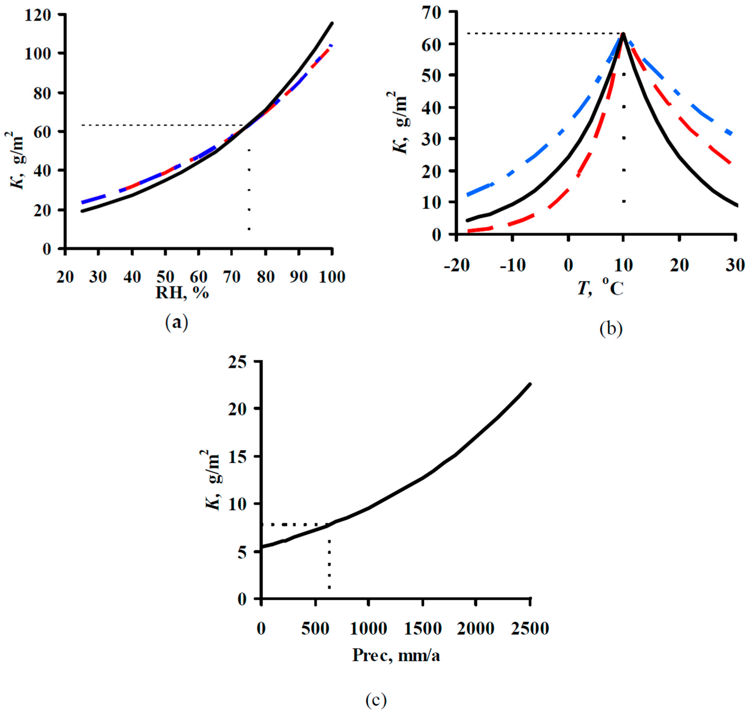
Figure 8.
Zinc. UN/ECE program. K1 predictions by the New DRF (a); Standard DRF (b); and Unified DRF (c). ●—experimental K1 data; ■—K1 predictions. □—K1 predictions without taking [H+] into account (only for the Unified DRF). Thin lines show the calculation error (±30%). The numbers of the exposure sites are given in accordance with Table 2.

Figure 9.
Zinc. MICAT program. K1 predictions by the New DRF (a); Standard DRF (b); and Unified DRF (c). ●—experimental K1 data; ■—K1 predictions. Thin lines show the calculation error (± 30%). The numbers of the exposure sites are given in accordance with Table 3.
Figure 9.
Zinc. MICAT program. K1 predictions by the New DRF (a); Standard DRF (b); and Unified DRF (c). ●—experimental K1 data; ■—K1 predictions. Thin lines show the calculation error (± 30%). The numbers of the exposure sites are given in accordance with Table 3.

Figure 10.
Zinc. RF program. K1 predictions by the New DRF (a); Standard DRF (b); and Unified DRF (c). ●—experimental K1 data; ■—K1 predictions. Thin lines show the calculation error (±30%). The numbers of the exposure sites are given in accordance with Table 4.
Figure 10.
Zinc. RF program. K1 predictions by the New DRF (a); Standard DRF (b); and Unified DRF (c). ●—experimental K1 data; ■—K1 predictions. Thin lines show the calculation error (±30%). The numbers of the exposure sites are given in accordance with Table 4.


Figure 11.
Variation of K for zinc versus relative humidity (a), temperature (b) and Prec (c) with account for the values of the DRF coefficients. ▬▬ by the New DRF; ▬ ▬ by the Standard DRF; ▬•▬ by the Unified DRF.
Figure 11.
Variation of K for zinc versus relative humidity (a), temperature (b) and Prec (c) with account for the values of the DRF coefficients. ▬▬ by the New DRF; ▬ ▬ by the Standard DRF; ▬•▬ by the Unified DRF.


Table 1.
Countries, names, and codes of test locations.
| MICAT Project | UN/ECE Program | ||||
|---|---|---|---|---|---|
| Country | Test Location | Designation | Country | Test Location | Designation |
| Argentina | Villa Martelli | A2 | Czech Republic | Prague | CS1 |
| Argentina | Iguazu | A3 | Czech Republic | Kasperske Hory | CS2 |
| Argentina | San Juan | A4 | Czech Republic | Kopisty | CS3 |
| Argentina | La Plata | A6 | Finland | Espoo | FIN4 |
| Brasil | Caratinga | B1 | Finland | Ähtäri | FIN5 |
| Brasil | Sao Paulo | B6 | Finland | Helsinki Vallila | FIN6 |
| Brasil | Belem | B8 | Germany | Waldhof Langenbrügge | GER7 |
| Brasil | Brasilia | B10 | Germany | Aschaffenburg | GER8 |
| Brasil | Paulo Afonso | B11 | Germany | Langenfeld Reusrath | GER9 |
| Brasil | Porto | B12 | Germany | Bottrop | GER10 |
| Colombia | San Pedro | CO2 | Germany | Essen Leithe | GER11 |
| Colombia | Cotove | CO3 | Germany | Garmisch Partenkirchen | GER12 |
| Ecuador | Guayaquil | EC1 | Netherlands | Eibergen | NL18 |
| Ecuador | Riobamba | EC2 | Netherlands | Vredepeel | NL19 |
| Spain | Leon | E1 | Netherlands | Wijnandsrade | NL20 |
| Spain | Tortosa | E4 | Norway | Oslo | NOR21 |
| Spain | Granada | E5 | Norway | Birkenes | NOR23 |
| Spain | Arties | E8 | Sweden | Stockholm South | SWE24 |
| Mexico | Mexico (a) | M1 | Sweden | Stockholm Centre | SWE25 |
| Mexico | Mexico (b) | M2 | Sweden | Aspvreten | SWE26 |
| Mexico | Cuernavaca | M3 | Spain | Madrid | SPA31 |
| Mexico | San Luis Potosi | PE4 | Spain | Toledo | SPA33 |
| Peru | Arequipa | PE5 | Russian Federation | Moscow | RUS34 |
| Peru | Arequipa | PE6 | Estonia | Lahemaa | EST35 |
| Peru | Pucallpa | U1 | Canada | Dorset | CAN37 |
| Uruguay | Trinidad | U3 | USA | Research Triangle Park | US38 |
| - | - | - | USA | Steubenville | US39 |
Table 2.
Atmosphere corrosivity parameters of test locations, first-year corrosion losses of carbon steel and zinc (K1, g/m2) under the UN/ECE program, and numbers of test locations in the order of increasing K1.
Table 2.
Atmosphere corrosivity parameters of test locations, first-year corrosion losses of carbon steel and zinc (K1, g/m2) under the UN/ECE program, and numbers of test locations in the order of increasing K1.
| Designation | T, °C | RH, % | TOW, Hours/a | Prec, mm/a | [SO2], μg/m3 | [H+], mg/L | Steel | Zinc | ||
|---|---|---|---|---|---|---|---|---|---|---|
| g/m2 | No. | g/m2 | No. | |||||||
| CS1 | 9.5 | 79 | 2830 | 639.3 | 77.5 | - | 438.0 | 76 | 14.89 | 92 |
| CS1 | 10.3 | 74 | 2555 | 380.8 | 58.1 | 0.0221 | - | - | 6.98 | 45 |
| CS1 | 9.1 | 73 | 2627 | 684.3 | 41.2 | 0.0714 | 270.7 | 64 | 7.78 | 53 |
| CS1 | 9.8 | 77 | 3529 | 581.1 | 32.1 | 0.0342 | 241.0 | 58 | 5.69 | 31 |
| CS2 | 7.0 | 77 | 3011 | 850.2 | 19.7 | - | 224.0 | 51 | 8.95 | 65 |
| CS2 | 7.4 | 76 | 3405 | 703.4 | 25.6 | 0.045 | - | - | 7.99 | 58 |
| CS2 | 6.6 | 73 | 2981 | 921 | 17.9 | 0.1921 | 152.9 | 33 | 6.77 | 44 |
| CS2 | 7.2 | 74 | 3063 | 941.2 | 12.2 | 0.0366 | 148.2 | 30 | 3.46 | 4 |
| CS3 | 9.6 | 73 | 2480 | 426.4 | 83.3 | - | 557.0 | 77 | 16.41 | 94 |
| CS3 | 9.9 | 72 | 2056 | 416.6 | 78.4 | 0.0242 | - | - | 11.59 | 87 |
| CS3 | 8.9 | 71 | 2866 | 431.6 | 49 | 0.058 | 350.2 | 73 | 11.74 | 88 |
| CS3 | 9.7 | 75 | 2759 | 512.7 | 49.2 | 0.0567 | 351.8 | 74 | 12.17 | 89 |
| FIN4 | 5.9 | 76 | 3322 | 625.9 | 18.6 | - | 271.0 | 63 | - | - |
| FIN4 | 6.4 | 80 | 4127 | 657 | 13.9 | 0.0392 | - | - | 8.42 | 62 |
| FIN4 | 5.6 | 79 | 3446 | 754.6 | 2.3 | 0.0231 | 130.3 | 21 | 5.18 | 25 |
| FIN4 | 6.0 | 80 | 3607 | 698.1 | 2.6 | 0.0334 | 120.9 | 20 | 4.68 | 19 |
| FIN5 | 3.1 | 78 | 2810 | 801.3 | 6.3 | - | 132.0 | 23 | 8.92 | 66 |
| FIN5 | 3.9 | 80 | 3342 | 670.7 | 1.8 | 0.0271 | - | - | 7.70 | 52 |
| FIN5 | 3.4 | 81 | 2994 | 609.7 | 0.9 | 0.0201 | 48.4 | 4 | 6.62 | 41 |
| FIN5 | 3.9 | 83 | 3324 | 675.4 | 0.8 | 0.0247 | 59.3 | 5 | 4.61 | 16 |
| FIN6 | 6.3 | 78 | 3453 | 673.1 | 20.7 | - | 273.0 | 65 | - | - |
| FIN6 | 6.8 | 80 | 4017 | 665.6 | 15.3 | 0.0554 | - | - | 9.29 | 70 |
| FIN6 | 6.2 | 78 | 3360 | 702.4 | 4.8 | 0.0221 | 162.2 | 34 | 5.69 | 33 |
| FIN6 | 6.6 | 76 | 3288 | 649.2 | 5.5 | 0.0139 | 195.8 | 44 | 5.62 | 30 |
| GER7 | 9.3 | 80 | 4561 | 630.6 | 13.7 | - | 264.0 | 62 | - | - |
| GER7 | 10.2 | 80 | 4390 | 499.7 | 11 | 0.0358 | - | - | 7.85 | 56 |
| GER7 | 8.9 | 81 | 4382 | 624.4 | 8.2 | 0.0342 | 230.9 | 53 | 9.07 | 68 |
| GER7 | 9.5 | 81 | 4676 | 595.6 | 3.9 | 0.0265 | 166.1 | 36 | 4.25 | 13 |
| GER8 | 12.3 | 77 | 4282 | 626.9 | 23.7 | - | 213.0 | 48 | - | - |
| GER8 | 12.2 | 67 | 2541 | 655.4 | 14.2 | 0.0411 | - | - | 4.68 | 18 |
| GER8 | 11.4 | 64 | 3563 | 561.2 | 12.6 | 0.0183 | 116.2 | 17 | 5.18 | 26 |
| GER8 | 11.6 | 65 | 2359 | 779 | 9.6 | - | 141.2 | 27 | 4.10 | 12 |
| GER9 | 10.8 | 77 | 4220 | 782.9 | 24.5 | - | 293.0 | 69 | - | - |
| GER9 | 11.7 | 80 | 4940 | 697.6 | 20.3 | 0.0366 | - | - | 6.62 | 40 |
| GER9 | 10.7 | 79 | 4437 | 619.1 | 16.3 | 0.0291 | 230.9 | 54 | 9.07 | 69 |
| GER9 | 11.4 | 81 | 5210 | 841 | 11.1 | 0.0278 | 209.8 | 47 | 7.63 | - |
| GER10 | 11.2 | 75 | 4077 | 873.8 | 50.6 | - | 373.0 | 75 | - | - |
| GER10 | 12 | 76 | 4107 | 696.6 | 48.5 | 0.0253 | - | - | 10.66 | 81 |
| GER10 | 10.3 | 78 | 4201 | 707.3 | 41.6 | 0.0211 | 347.1 | 72 | 15.34 | 93 |
| GER10 | 11.8 | 80 | 4930 | 912.9 | 30.2 | 0.0334 | 294.1 | 70 | 7.85 | 55 |
| GER11 | 10.5 | 79 | 4537 | 713.1 | 30.3 | - | 342.0 | 71 | - | - |
| GER11 | 11.5 | 77 | 4040 | 644.5 | 25.6 | 0.042 | - | - | 9.72 | 73 |
| GER11 | 10.1 | 79 | 4120 | 683.6 | 22.9 | 0.0253 | 293.3 | 68 | 11.45 | 86 |
| GER11 | 10.9 | 78 | 4632 | 889.3 | 16.2 | 0.0247 | 241.0 | 57 | 7.06 | 46 |
| GER12 | 8.0 | 82 | 4989 | 1491.5 | 9.4 | - | 133.0 | 24 | 8.35 | 61 |
| GER12 | 7.3 | 82 | 4201 | 1183.1 | 6.1 | 0.0171 | - | - | 7.27 | 49 |
| GER12 | 7.1 | 84 | 4545 | 1552.4 | 3.2 | 0.0018 | 89.7 | 9 | 7.20 | 48 |
| GER12 | 7.4 | 83 | 4375 | 1503 | 2.4 | - | 85.0 | 8 | 3.74 | 9 |
| NL18 | 9.9 | 83 | 5459 | 904.2 | 10.1 | - | 232.0 | 55 | 9.93 | 76 |
| NL18 | 10.9 | 79 | 4482 | 705.9 | 8.5 | 0.0046 | - | - | 8.14 | 59 |
| NL18 | 9.5 | 82 | 4808 | 872.8 | 7.4 | 0.004 | 204.4 | 45 | 7.92 | 57 |
| NL18 | 10.3 | 83 | 5358 | 987.1 | 4.7 | 0.0366 | 144.3 | 28 | 4.75 | 20 |
| NL19 | 10.3 | 81 | 5354 | 845 | 13 | - | 283.0 | 66 | - | - |
| NL19 | 11 | 81 | 4969 | 569.1 | 9.9 | 0.0049 | - | - | 9.07 | 67 |
| NL19 | 10 | 82 | 5084 | 749.2 | 8.3 | 0.0021 | 238.7 | 56 | 11.09 | 84 |
| NL19 | 10.9 | 83 | 5454 | 828.9 | 4.5 | - | 180.2 | 39 | - | - |
| NL20 | 10.3 | 81 | 5125 | 801.3 | 13.7 | - | 259.0 | 59 | - | - |
| NL20 | 11.1 | 77 | 4424 | 608.8 | 10.3 | 0.0106 | - | - | 10.22 | 77 |
| NL20 | 10.1 | 81 | 4688 | 679.6 | 9.3 | 0.0113 | 205.1 | 46 | 11.38 | 85 |
| NL20 | 11.1 | 82 | 5141 | 789.9 | 5.8 | 0.0038 | 172.4 | 37 | 6.34 | 37 |
| NOR21 | 7.6 | 70 | 2673 | 1023.8 | 14.4 | - | 229.0 | 52 | - | - |
| NOR21 | 8.8 | 70 | 2864 | 526.6 | 7.9 | 0.0326 | - | - | 5.69 | 32 |
| NOR21 | 7.7 | 68 | 2471 | 440.1 | 6 | 0.0156 | 134.9 | 25 | 6.70 | 43 |
| NOR21 | 7.5 | 69 | 2827 | 680 | 2.9 | 0.0136 | 100.6 | 11 | 3.53 | 7 |
| NOR23 | 6.5 | 80 | 4831 | 2144.3 | 1.3 | - | 194.0 | 43 | - | - |
| NOR23 | 7.4 | 77 | 4193 | 1762.2 | 0.9 | 0.042 | - | - | 8.50 | 63 |
| NOR23 | 5.9 | 75 | 3341 | 1188.6 | 0.7 | 0.0374 | 131.8 | 22 | 10.58 | 80 |
| NOR23 | 6.4 | 76 | 3779 | 1419.7 | 0.7 | 0.0326 | 109.2 | 15 | 5.04 | 24 |
| SWE24 | 7.6 | 78 | 3959 | 531 | 16.8 | - | 264.0 | 61 | 10.36 | 79 |
| SWE24 | 8.7 | 70 | 3074 | 473.2 | 8.4 | 0.0366 | - | - | 6.12 | 35 |
| SWE24 | 7 | 70 | 2580 | 577 | 5.7 | 0.043 | 120.1 | 18 | 4.54 | 15 |
| SWE24 | 7.5 | 73 | 3160 | 580.6 | 4.2 | 0.0231 | 103.0 | 13 | 4.25 | 14 |
| SWE25 | 7.6 | 78 | 3959 | 531 | 19.6 | - | 263.0 | 60 | 9.76 | 74 |
| SWE25 | 8.7 | 70 | 3074 | 473.2 | 10.3 | 0.0366 | - | - | 5.62 | 29 |
| SWE25 | 7 | 70 | 2580 | 577 | 4.7 | 0.043 | 103.0 | 12 | 3.53 | 5 |
| SWE25 | 7.5 | 73 | 3160 | 580.6 | 3.4 | 0.0231 | 95.2 | 10 | 3.53 | 8 |
| SWE26 | 6.0 | 83 | 4534 | 542.7 | 3.3 | - | 147.0 | 29 | 8.31 | 60 |
| SWE26 | 7.6 | 77 | 3469 | 342.3 | 2 | 0.043 | - | - | 6.70 | 42 |
| SWE26 | 6 | 81 | 3592 | 467.8 | 1.3 | 0.043 | 74.9 | 6 | 4.90 | 23 |
| SWE26 | 6.8 | 82 | 4118 | 525.2 | 1.1 | 0.0278 | 81.1 | 7 | 6.05 | 34 |
| SPA31 | 14.1 | 66 | 2762 | 398 | 18.4 | - | 222.0 | 50 | 7.74 | 54 |
| SPA31 | 15.2 | 56 | 1160 | 331.5 | 15.3 | 0.0073 | - | - | 4.82 | 22 |
| SPA31 | 14.3 | 67 | 2319 | 360.1 | 8.2 | 0.0003 | 162.2 | 35 | 3.53 | 6 |
| SPA31 | 15.7 | 68 | 2766 | 223.9 | 7.8 | 0.0002 | 151.3 | 32 | 2.30 | 2 |
| SPA33 | 14.0 | 64 | 2275 | 785 | 3.3 | - | 45.0 | 3 | 3.37 | 3 |
| SPA33 | 15.5 | 61 | 2147 | 610.4 | 13.5 | 0.0006 | - | - | 3.89 | 11 |
| SPA33 | 13.4 | 61 | 1888 | 432.5 | 1.7 | 0.0012 | 25.7 | 1 | 3.89 | 10 |
| SPA33 | 14.8 | 57 | 1465 | 327.4 | 4.2 | 0.0006 | 35.9 | 2 | 1.66 | 1 |
| RUS34 | 5.5 | 73 | 2084 | 575.4 | 19.2 | - | 181.0 | 40 | 10.32 | 78 |
| RUS34 | 5.7 | 76 | 2894 | 860.2 | 30.8 | 0.0006 | - | - | 8.64 | 64 |
| RUS34 | 5.7 | 74 | 2444 | 880.6 | 28.7 | 0.0009 | 141.2 | 26 | 6.48 | 39 |
| RUS34 | 5.6 | 71 | 1514 | 666.7 | 16.4 | 0.0008 | 120.9 | 19 | 4.61 | 17 |
| EST35 | 5.5 | 83 | 4092 | 447.8 | 0.9 | - | 185.0 | 41 | 7.18 | 47 |
| EST35 | 6.7 | 81 | 4332 | 532.7 | 0.6 | 0.0226 | - | - | 9.43 | 71 |
| CAN37 | 5.5 | 75 | 3252 | 961.1 | 3.3 | - | 149.0 | 31 | 9.88 | 75 |
| CAN37 | 5 | 79 | 3431 | 1103 | 3 | 0.042 | - | - | 6.26 | 38 |
| CAN37 | 4.3 | 80 | 3302 | 1080 | 2.1 | 0.0482 | 110.0 | 16 | 5.26 | 27 |
| CAN37 | 5.2 | 80 | 3386 | 1022.8 | 3.3 | 0.0461 | 103.7 | 14 | 6.19 | 36 |
| US38 | 14.6 | 69 | 3178 | 846.7 | 9.6 | - | 176.0 | 38 | 10.72 | 82 |
| US38 | 16.3 | 66 | 3026 | 1106.7 | 9.2 | 0.0358 | - | - | 12.46 | 90 |
| US38 | 15.5 | 64 | 2644 | 982.3 | 10.1 | 0.0349 | 184.9 | 42 | 9.72 | 72 |
| US38 | 15.8 | 68 | - | 1037.6 | 9.3 | 0.0482 | - | - | 4.75 | 21 |
| US39 | 12.3 | 67 | 2111 | 733.1 | 58.1 | - | 214.0 | 49 | 13.61 | 91 |
| US39 | 11.2 | 61 | 1391 | 967.4 | 55.2 | 0.0838 | - | - | 11.02 | 83 |
| US39 | 11.8 | 65 | 1532 | 729.4 | 43.1 | 0.0941 | 290.2 | 67 | 7.34 | 50 |
| US39 | 11.8 | 69 | - | 756.8 | 38.3 | 0.0765 | - | - | 5.26 | 28 |
Table 3.
Atmosphere corrosivity parameters of test locations, first-year corrosion losses of carbon steel and zinc (K1, g/m2) under the MICAT program and those reported in [20], and numbers of test locations in the order of increasing K1. Adapted from [20], with permission from © 2000 Elsevier.
| Designation | T, °C | RH, % | Rain, mm/a | [SO2], μg/m3 | Cl−, mg/(m2·Day) | TOW, h/a | Steel | Zinc | ||
|---|---|---|---|---|---|---|---|---|---|---|
| g/m2 | No. | g/m2 | No. | |||||||
| A2 * | 16.7 | 75 | 1729 | 10 | Ins | 5063 | 122.5 | 36 (34) | 8.06 | 41 |
| A2 | 17.1 | 72 | 983 | 10 | Ins | 4222 | 125.6 | 38 | 7.56 | 39 |
| A2 | 17.0 | 74 | 1420 | 9 | Ins | 4862 | 96.7 | 25 | 10.15 | 47 |
| A3 | 20.6 | 76 | 2158 | Ins (5) ** | Ins (1.5) | 5825 | 44.5 | 12 (11) | 14.76 | 53 |
| A3 | 20.9 | 74 | 2624 | Ins (5) | Ins (1.5) | 5528 | 45.2 | 13 (12) | 8.42 | 43 |
| A3 | 22.1 | 75 | 1720 | Ins (5) | Ins (1.5) | 5545 | 43.7 | 10 (9) | 8.50 | 44 |
| A4 | 18.0 | 51 | 35 | Ins (5) | Ins (1.5) | 999 | 35.9 | 6 (6) | 2.02 | 15 |
| A4 | 20.0 | 49 | 111 | Ins (5) | Ins (1.5) | 850 | 35.1 | 5 (5) | 0.94 | 3 |
| A4 | 18.3 | 51 | 93 | Ins (5) | Ins (1.5) | 867 | 43.7 | 11 (10) | 1.58 | 10 |
| A6 | 17.0 | 78 | 1178 | 6.22 | Ins | 5195 | 197.3 | 55 (51) | 5.54 | 28 |
| A6 * | 16.7 | 77 | 1263 | 8.21 | Ins | 4949 | 224.6 | 59 (55) | 6.70 | 32 |
| A6 * | 16.6 | 78 | 1361 | 6.2 | Ins | 5528 | 234.8 | 61 (57) | 7.49 | 37 |
| B1 | 21.2 | 75 | 996 | 1.67 | 1.57 | 4222 | 102.2 | 28(26) | 4.32 | 26 |
| B6 | 19.7 | 75 | 1409 | 67.2 (28) | Ins (1.5) | 5676 | 113.9 | 31 (29) | 8.57 | 45 |
| B6 | 19.5 | 76 | 1810 (1910) | 66.8 (28) | Ins (1.5) | 5676 | 182.5 | 53 (49) | 10.66 | 48 |
| B6 | 19.6 | 75 | 1034 | 48.8 (28) | Ins (1.5) | 5676 | 188.8 | 54 (50) | 6.98 | 34 |
| B8 | 26.1 | 88 | 2395 | Ins (5) | Ins (1.5) | 5974 | 151.3 | 44 (40) | 7.92 | 40 |
| B10 | 20.4 | 69 (72) | 1440 | Ins (5) | Ins (1.5) | 3872 | 100.6 | 26 (24) | 12.82 | 50 |
| B11 | 25.9 | 77 | 1392 | Ins | Ins | 1507 | 134.9 | 41 | 11.52 | 49 |
| B12 | 26.6 | 90 | 2096 | Ins | Ins | 4222 | 38.2 | 8 | 23.83 | 57 |
| CO2 | 9.6 (14.1) | 98 (81) | 1800 | 0.56 (5) | Ins (1.5) | 8760 (7008) | 106.9 | 30 (28) | 24.48 | 58 |
| CO2 | 11.4 | 90 | 1800 | 0.56 (5) | Ins (1.5) | 8760 (7808) | 138.1 | 42 (38) | 25.78 | 60 |
| CO2 | 13.5 (14.2) | 81 (73) | 1800 | 0.56 (5) | Ins (1.5) | 8760 (7808) | 152.9 | 46 (42) | 20.88 | 55 |
| CO3 * | 27.0 | 76 | 900 | 0.33 | Ins | 2891 | 120.9 | 35 (33) | 18.65 | 54 |
| CO3 * | 27.0 | 76 | 900 | 0.33 | Ins | 2891 | 204.4 | 57 (53) | 27.00 | 61 |
| CO3 * | 27.0 | 76 | 900 | 0.33 | Ins | 2891 | 132.6 | 40 (37) | 25.56 | 59 |
| EC1 | 26.1 | 71 | 936 | 4.20 | 1.5 | 4853 | 152.1 | 45 (41) | 1.08 | 5 |
| EC1 | 26.9 | 82 | 635 | 2.72 | 1.31 | 5790 | 176.3 | 52 (48) | 1.15 | 6 |
| EC1 * | 24.8 | 75 | 564 | 2.1 | 1.66 | 3101 | 201.2 | 56 (52) | 2.38 | 17 |
| EC2 | 12.9 | 66 | 554 | 1.0 | 0.4 | 3583 | 60.8 | 17 (16) | - | - |
| EC2 * | 13.2 | 71 | 598 | 1.35 | 1.14 | 4932 | 70.2 | 21 (20) | - | - |
| E1 | 12.0 | 69 | 652 | 1.18 (16.2) | 1.5 | 3364 | 158.3 (150.5) | 48 (44) | 3.02 | 20 |
| E1 * | 10.6 | 65 | 495 | 1.18 | 1.5 | 2374 | 175.5 | 51 (47) | 2.88 | 18 |
| E1 | 11.1 | 63 | 334 | 1.18 (16.2) | 1.5 | 2111 | 153.7 | 47 (43) | 2.09 | 16 |
| E4 | 18.1 | 65 | 554 | 8.3 | 1.5 | 3416 | 158.3 | 49 (45) | 1.94 | 14 |
| E4 | 17.0 | 63 | 521 | 5.7 | 1.5 | 2646 | 151.3 | 43 (39) | 1.51 | 8 |
| E4 | 17.2 | 62 | 374 | 1.9 | 1.5 | 2768 | 163.8 | 50 (46) | 1.94 | 13 |
| E5 | 16.3 | 59 | 416 | 10.3 | 1.5 | 1323 | 95.9 | 24 (23) | 1.01 | 4 |
| E5 | 15.0 (15.8) | 59 (58) | 258 (239) | 5.4 | 1.5 | 1104 | 53.0 | 16 (15) | 0.65 | 2 |
| E5 | 15.6 | 58 | 266 | 2.8 | 1.5 | 2400 | 49.9 | 15 (14) | 0.65 | 1 |
| E8 | 8.8 | 52 (72) | 738 | 9.1 | 1.8 | 876 | 25.7 | 3 (3) | 1.66 | 11 |
| E8 | 6.9 | 52 (72) | 624 | 8.9 | 1.6 | 876 | 28.1 | 4 (4) | 1.22 | 7 |
| E8 | 7.8 | 52 (72) | 681 | 9.0 | 1.7 | 876 | 37.4 | 7 (7) | 3.10 | 21 |
| M1 | 16.0 | 62 | 743 | 15.6 | 1.5 | 2523 (2321) | 120.1 | 34 (32) | 5.83 | 29 |
| M1 | 14.8 (15.2) | 66 (65) | 747 | 7.7 (5.6) | 1.5 | 2523 | 67.1 | 20 (19) | 5.98 | 31 |
| M1 | 15.4 | 64 (63) | 747 | 17.5 | 1.5 | 2523 (2427) | 39.8 | 9 (8) | 5.83 | 30 |
| M2 | 21.0 | 56 | 1352 | 6.7 | 1.5 | 1664 | 118.6 | 33 (31) | 8.35 | 42 |
| M2 | 21.0 | 56 | 1724 | 9.9 | Ins (1.5) | 1857 | 88.9 | 22 (21) | 14.33 | 52 |
| M2 | 21.0 | 56 | 1372 | 7.1 | Ins (1.5) | 1752 | 106.9 | 29 (27) | 6.84 | 33 |
| M3 | 18.0 | 51 | 374 | 31.1 | Ins | 1410 | 292.5 | 62 (58) | 10.01 | 46 |
| M3 * | 18.0 | 62 | 374 | 10.9 | Ins | 1410 | 205.9 | 58 (54) | 21.24 | 56 |
| M3 * | 18.0 | 60 | 374 | 14.6 | Ins | 2646 | 229.3 | 60 (56) | 7.06 | 35 |
| PE4 | 16.4 | 37 | 17 | Ins (5) | Ins (1.5) | 26 | 117.0 | 32 (30) | 1.66 | 12 |
| PE4 | 17.2 | 33 | 34 (89) | Ins (5) | Ins (1.5) | 175 (26) | 128.7 | 39 (36) | 1.58 | 9 |
| PE5 | 12.2 | 67 | 632 | Ins (0) | Ins (0) | 2847 | 7.8 | 1 (1) | 3.89 | 23 |
| PE5 | 12.2 | 67 | 672 (792) | Ins (0) | Ins (0) | 2689 (2847) | 13.3 | 2 (2) | 2.88 | 19 |
| PE6 | 25.4 | 84 | 1523 | Ins (5) | Ins (1.5) | 5037 (4580) | 122.5 | 37 (35) | 7.06 | 36 |
| PE6 | 25.8 | 83 | 1158 (1656) | Ins (5) | Ins (1.5) | 5790 (4380) | 100.6 | 27 (25) | 7.49 | 38 |
| U1 | 16.8 | 74 | 1182 | 0.6 (1) | 1.8 (2.2) | 5133 | 64.0 | 19 (18) | 4.03 | 24 |
| U1 * | 16.6 | 73 | 1324 | 0.8 | 1.2 | 4976 | 62.4 | 18 (17) | 3.74 | 22 |
| U1 * | 16.7 | 76 | 1306 | Ins | Ins | 4792 | 47.6 | 14 (13) | 4.10 | 25 |
| U3 * | 17.7 | 79 | 1490 | Ins | Ins | 5764 | 94.4 | 23 (22) | 4.39 | 27 |
| CH1 | 14.2 | 71 | 355 | 20 | 2.18 | 3469 | 221.5 | 63 | 12.89 | 51 |
Table 4.
Atmosphere corrosivity parameters of test locations and first-year corrosion losses of carbon steel and zinc (K1, g/m2) in Russian Federation test locations and their numbers in the order of increasing K1.
Table 4.
Atmosphere corrosivity parameters of test locations and first-year corrosion losses of carbon steel and zinc (K1, g/m2) in Russian Federation test locations and their numbers in the order of increasing K1.
| Test Location | T, °C | RH, % | Prec, mm/a | [SO2], μg/m3 | Steel | Zinc | ||
|---|---|---|---|---|---|---|---|---|
| g/m2 | No. | g/m2 | No. | |||||
| Bilibino | −12.2 | 80 | 218 | 3 | 5.4 | 1 | 1.64 | 1 |
| Oimyakon | −16.6 | 71 | 175 | 3 | 8.1 | 2 | 1.81 | 3 |
| Ust-Omchug | −11 | 70 | 317 | 5 | 12.4 | 3 | 2.91 | 5 |
| Atka | −12 | 72 | 376 | 3 | 15.2 | 4 | 1.69 | 2 |
| Susuman | −13.2 | 71 | 283 | 10 | 17.0 | 5 | 3.07 | 6 |
| Tynda | −6.5 | 72 | 525 | 5 | 21.2 | 6 | 5.30 | 10 |
| Klyuchi | 1.4 | 69 | 253 | 3 | 23.4 | 7 | 2.03 | 4 |
| Aldan | −6.2 | 72 | 546 | 5 | 24.6 | 8 | 5.47 | 11 |
| Pobedino | −0.9 | 77 | 604 | 3 | 36.5 | 9 | 4.30 | 7 |
| Yakovlevka | 2.5 | 70 | 626 | 3 | 40.6 | 10 | 4.64 | 9 |
| Pogranichnyi | 3.6 | 67 | 595 | 3 | 49.0 | 11 | 4.32 | 8 |
| Komsomolsk-on-Amur | −0.7 | 76 | 499 | 10 | 63.2 | 12 | 6.35 | 12 |
Table 5.
Atmosphere corrosivity parameters and first-year corrosion losses of carbon steel in test locations. Adapted from [19], with permission from © 1999 Elsevier.
Table 5.
Atmosphere corrosivity parameters and first-year corrosion losses of carbon steel in test locations. Adapted from [19], with permission from © 1999 Elsevier.
| [SO2], μg/m3 | Cl−, mg/(m2·Day) | K1, g/m2 |
|---|---|---|
| 3 | 2 | 137.7 |
| 5 | 0,3 | 46.1 |
| 5 | 0,7 | 130.7 |
| 8 | 1 | 137.7 |
| 8 | 0 | 140.0 |
| 14 | 2 | 193.8 |
| 15 | 2 | 228.4 |
| 15 | 1 | 236.1 |
| 17 | 0,16 | 136.1 |
| 26 | 1 | 236.1 |
| 32 | 2 | 276.1 |
| 116 | 0,62 | 232.2 |
Table 6.
Atmosphere corrosivity parameters and first year corrosion losses of carbon steel in certain test locations under the MICAT project.
Table 6.
Atmosphere corrosivity parameters and first year corrosion losses of carbon steel in certain test locations under the MICAT project.
| Locations with Uncertain Data | Locations with Trusted Data | ||||||||||||||||
|---|---|---|---|---|---|---|---|---|---|---|---|---|---|---|---|---|---|
| Designation | No. | T, °C | RH, % | TOW, 1/a | Prec, mm/a | [SO2], μg/m3 | K1exp | Designation | No. | T, °C | RH, % | TOW, 1/a | Prec, mm/a | [SO2], μg/m3 | K1exp | ||
| µm | g/m2 | µm | g/m2 | ||||||||||||||
| PE4 | 32 | 16.4 | 37 | 0.003 | 17 | 1 | 15.0 | 117.0 | E8 | 3 | 8.8 | 52 | 0.100 | 738 | 9.1 | 3.3 | 25.7 |
| PE4 | 39 | 17.2 | 33 | 0.020 | 34 | 1 | 16.5 | 128.7 | E8 | 4 | 6.9 | 52 | 0.100 | 624 | 8.9 | 3.6 | 28.1 |
| A4 | 5 | 20.0 | 49 | 0.097 | 111 | 1 | 4.5 | 35.1 | E8 | 7 | 7.8 | 52 | 0.100 | 681 | 9 | 4.8 | 37.4 |
| A4 | 6 | 18.0 | 51 | 0.114 | 35 | 1 | 4.6 | 35.9 | M2 | 29 | 21.0 | 56 | 0.200 | 1372 | 7.1 | 13.7 | 106.9 |
| M3 | 58 | 18.0 | 62 | 0.161 | 374 | 10.9 | 26.4 | 205.9 | M2 | 33 | 21.0 | 56 | 0.190 | 1352 | 6.7 | 15.2 | 118.6 |
| M3 | 62 | 18.0 | 51 | 0.161 | 374 | 31.1 | 37.5 | 292.5 | M2 | 22 | 21.0 | 56 | 0.212 | 1724 | 9.9 | 11.4 | 88.9 |
| M3 | 60 | 18.0 | 60 | 0.302 | 374 | 14.6 | 29.4 | 229.3 | E5 | 15 | 15.6 | 58 | 0.161 | 266 | 2.8 | 6.4 | 49.9 |
| E1 | 47 | 11.1 | 63 | 0.241 | 334 | 1.18 | 19.7 | 153.7 | E5 | 16 | 15.0 | 59 | 0.126 | 258 | 5.4 | 6.8 | 53.0 |
| E1 | 48 | 12.0 | 69 | 0.384 | 652 | 1.18 | 20.3 | 158.3 | M1 | 34 | 16.0 | 62 | 0.288 | 743 | 15.6 | 15.4 | 120.1 |
| E1 | 51 | 10.6 | 65 | 0.271 | 495 | 1.18 | 22.5 | 175.5 | M1 | 9 | 15.4 | 64 | 0.288 | 743 | 17.5 | 5.1 | 39.8 |
| E4 | 43 | 17.0 | 63 | 0.302 | 521 | 5.7 | 19.4 | 151.3 | M1 | 20 | 14.8 | 66 | 0.288 | 743 | 7.7 | 8.6 | 67.1 |
| E4 | 49 | 18.1 | 65 | 0.390 | 554 | 8.3 | 20.3 | 158.3 | A2 | 38 | 17.1 | 72 | 0.482 | 983 | 10.0 | 16.1 | 125.6 |
| E4 | 50 | 17.2 | 62 | 0.316 | 374 | 1.9 | 21.0 | 163.8 | A2 | 36 | 16.7 | 75 | 0.578 | 1729 | 10.0 | 15.7 | 122.5 |
| B10 | 26 | 20.4 | 69 | 0.442 | 1440 | 1 | 12.9 | 100.6 | A2 | 25 | 17.0 | 74 | 0.555 | 1420 | 9 | 12.4 | 96.7 |
| B1 | 28 | 21.2 | 75 | 0.484 | 996 | 1.67 | 13.1 | 102.2 | A3 | 12 | 20.6 | 76 | 0.665 | 2158 | 1 | 5.7 | 44.5 |
| CO3 | 40 | 27.0 | 76 | 0.330 | 900 | 1 | 17.0 | 132.6 | A3 | 13 | 20.9 | 74 | 0.631 | 2624 | 1 | 5.8 | 45.2 |
| CO3 | 57 | 27.0 | 76 | 0.330 | 900 | 1 | 26.2 | 204.4 | A3 | 10 | 22.1 | 75 | 0.633 | 1720 | 1 | 5.6 | 43.7 |
| B11 | 41 | 25.9 | 77 | 0.172 | 1392 | 1 | 17.3 | 134.9 | - | - | - | - | - | - | - | - | - |
| EC1 | 56 | 24.8 | 75 | 0.354 | 564 | 2.1 | 25.8 | 201.2 | - | - | - | - | - | - | - | - | - |
| EC1 | 52 | 26.9 | 82 | 0.661 | 635 | 2.72 | 22.6 | 176.3 | - | - | - | - | - | - | - | - | - |
Table 7.
Values of coefficients used in the nonlinear DRFs for carbon steel.
| DRF | A | α | k1 | k2 | k3 | ||
|---|---|---|---|---|---|---|---|
| µm | g/m2 | T ≤ 10 | T > 10 | ||||
| New | 0.99 | 7.7 | 0.47 | 0.024 | 0.095 | −0.095 | 0.00056 |
| Standard | 1.77 | 13.8 | 0.52 | 0.020 | 0.150 | −0.054 | - |
| Unified | 3.54 | 27.6 | 0.13 | 0.020 | 0.059 | −0.036 | - |
Table 8.
Values of coefficients used in the nonlinear DRFs for zinc.
| DRF | A | α | k1 | k2 | k3 | B | |||
|---|---|---|---|---|---|---|---|---|---|
| µm | g/m2 | T ≤ 10 | T > 10 | µg | g/m2 | ||||
| New | 0.0986 | 0.71 | 0.28 | 0.022 | 0.045 | −0.085 | 0.0001 | - | - |
| Standard | 0.0129 | 0.0929 | 0.44 | 0.046 | 0.038 | −0.071 | - | - | - |
| Unified | 0.188 | 1.35 | 0.22 | 0.018 | 0.062 | −0.021 | - | 0.00403 | 0.029 |
© 2017 by the authors. Licensee MDPI, Basel, Switzerland. This article is an open access article distributed under the terms and conditions of the Creative Commons Attribution (CC BY) license (http://creativecommons.org/licenses/by/4.0/).
Share and Cite
MDPI and ACS Style
Panchenko, Y.M.; Marshakov, A.I. Prediction of First-Year Corrosion Losses of Carbon Steel and Zinc in Continental Regions. Materials 2017, 10, 422. https://doi.org/10.3390/ma10040422
AMA Style
Panchenko YM, Marshakov AI. Prediction of First-Year Corrosion Losses of Carbon Steel and Zinc in Continental Regions. Materials. 2017; 10(4):422. https://doi.org/10.3390/ma10040422
Chicago/Turabian StylePanchenko, Yulia M., and Andrey I. Marshakov. 2017. "Prediction of First-Year Corrosion Losses of Carbon Steel and Zinc in Continental Regions" Materials 10, no. 4: 422. https://doi.org/10.3390/ma10040422
Note that from the first issue of 2016, this journal uses article numbers instead of page numbers. See further details here.