
Modelling of Fluidised Geomaterials: The Case of the Aberfan and the Gypsum Tailings Impoundment Flowslides

 , ,
, ,  ,
,
Abstract
:1. Introduction
2. Mathematical Model
2.1. Solid Skeleton Pore Fluid Coupled Mathematical Model
2.2. Depth-Integrated Mathematical Model
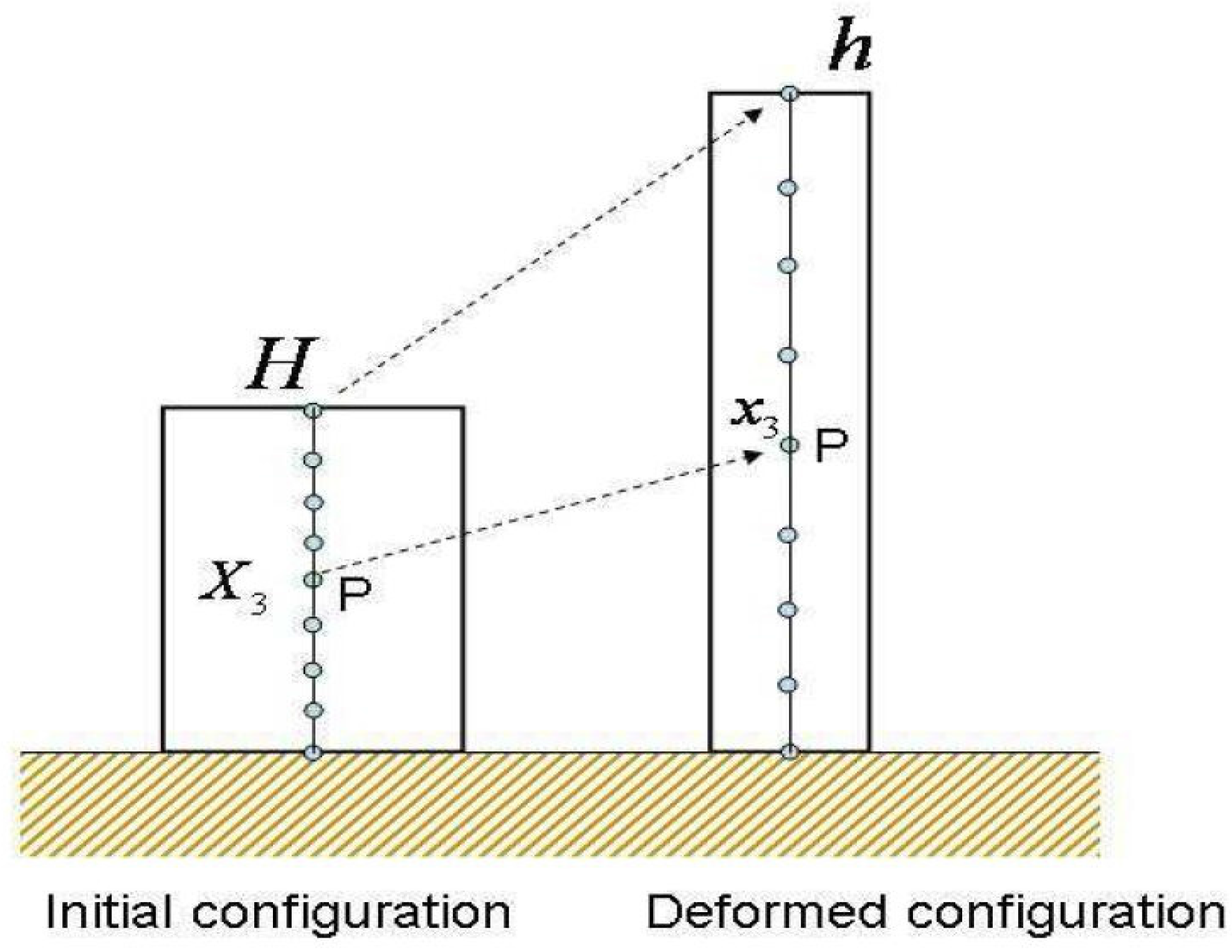
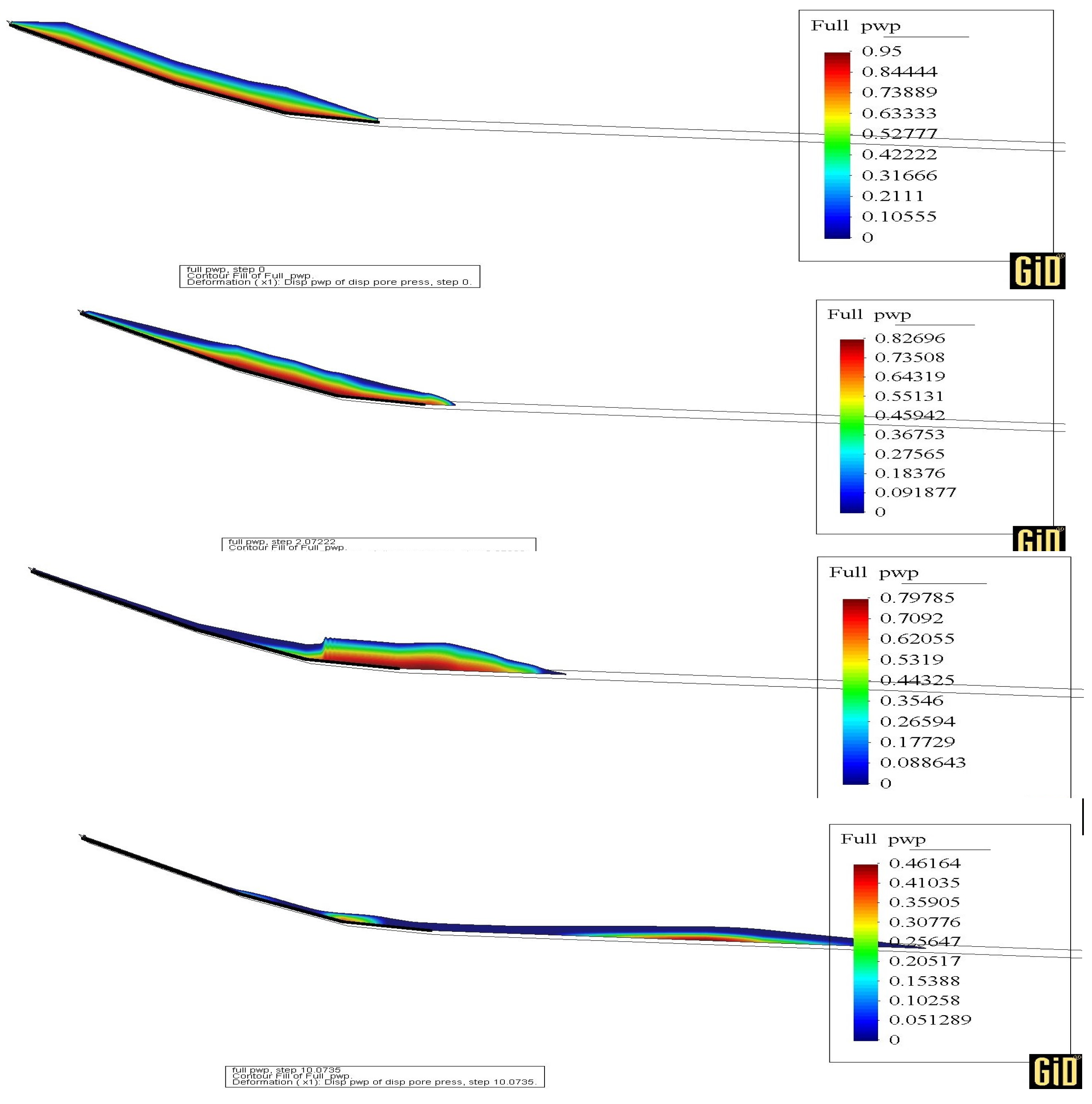
2.3. Pore Pressure Evolution in Landslides
- Depth-integrated equations
- A pore pressure evolution equation
3. Rheological Models for Fluidised Soils
3.1. Introduction
3.2. Pure Cohesive Viscoplastic Fluid: Bingham Model
3.3. Pure Frictional Viscoplastic Fluid
3.4. Perzyna-Based Rheological Model for Frictional Materials
4. Depth-Integrated SPH Model Coupled with a Finite Difference Scheme for Pore Pressure
5. Application
5.1. Introduction
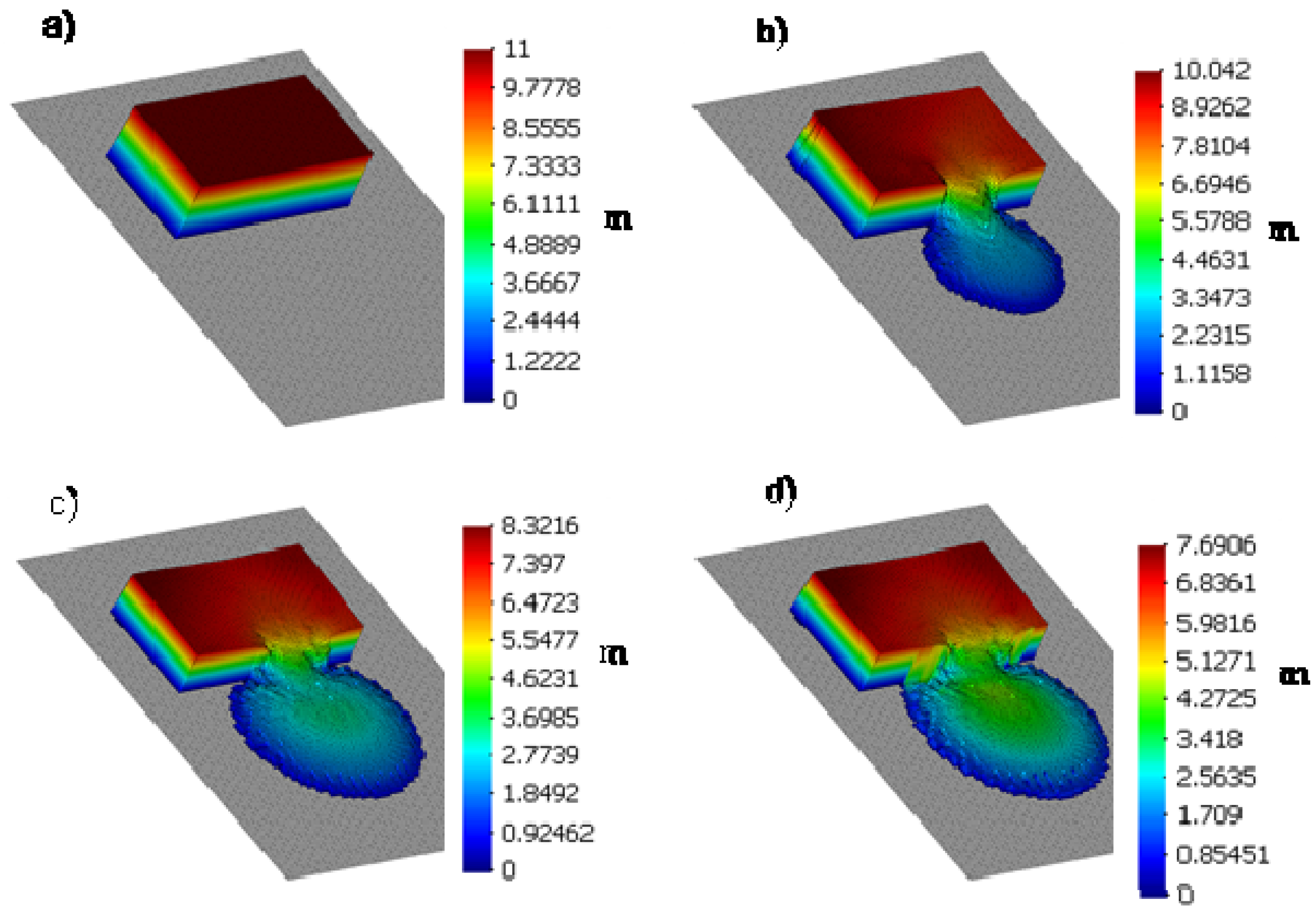
5.2. East Texas Gypsum Tailings Failure (1966)
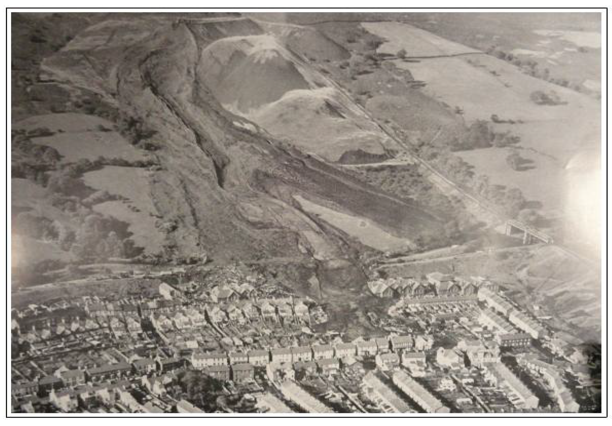
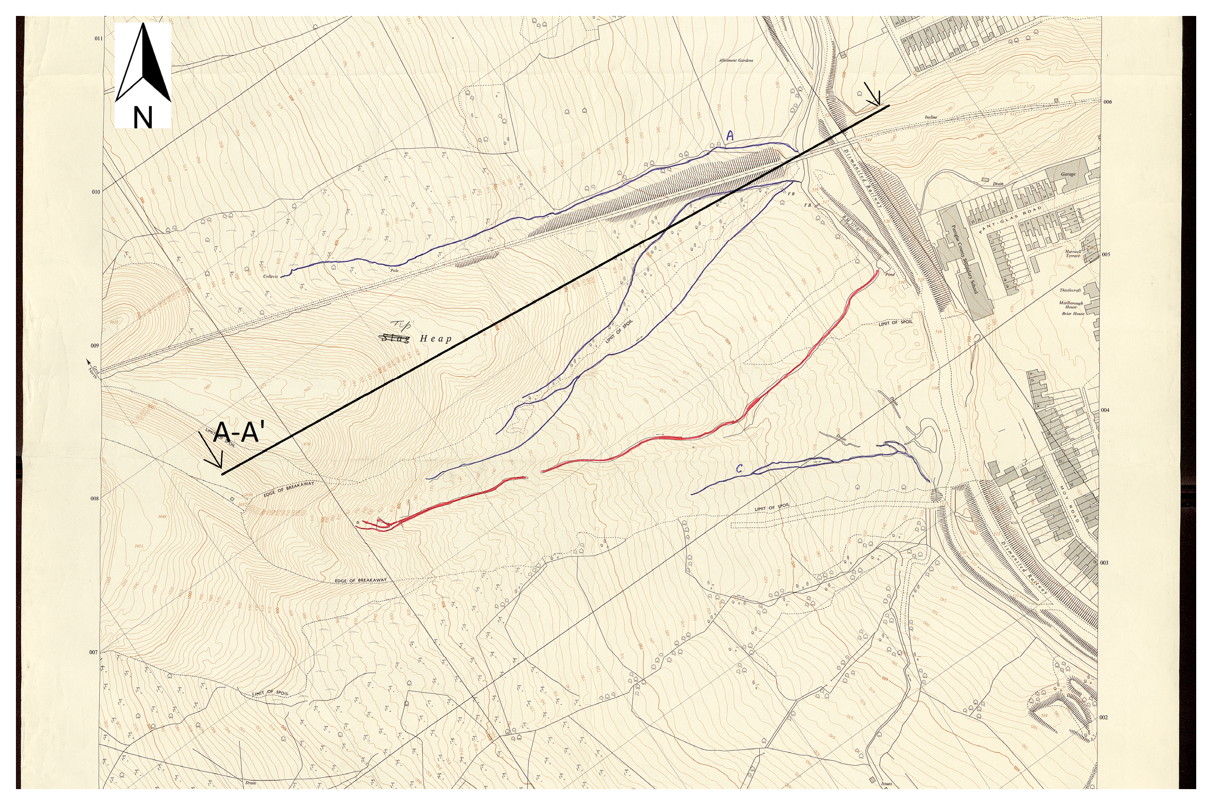
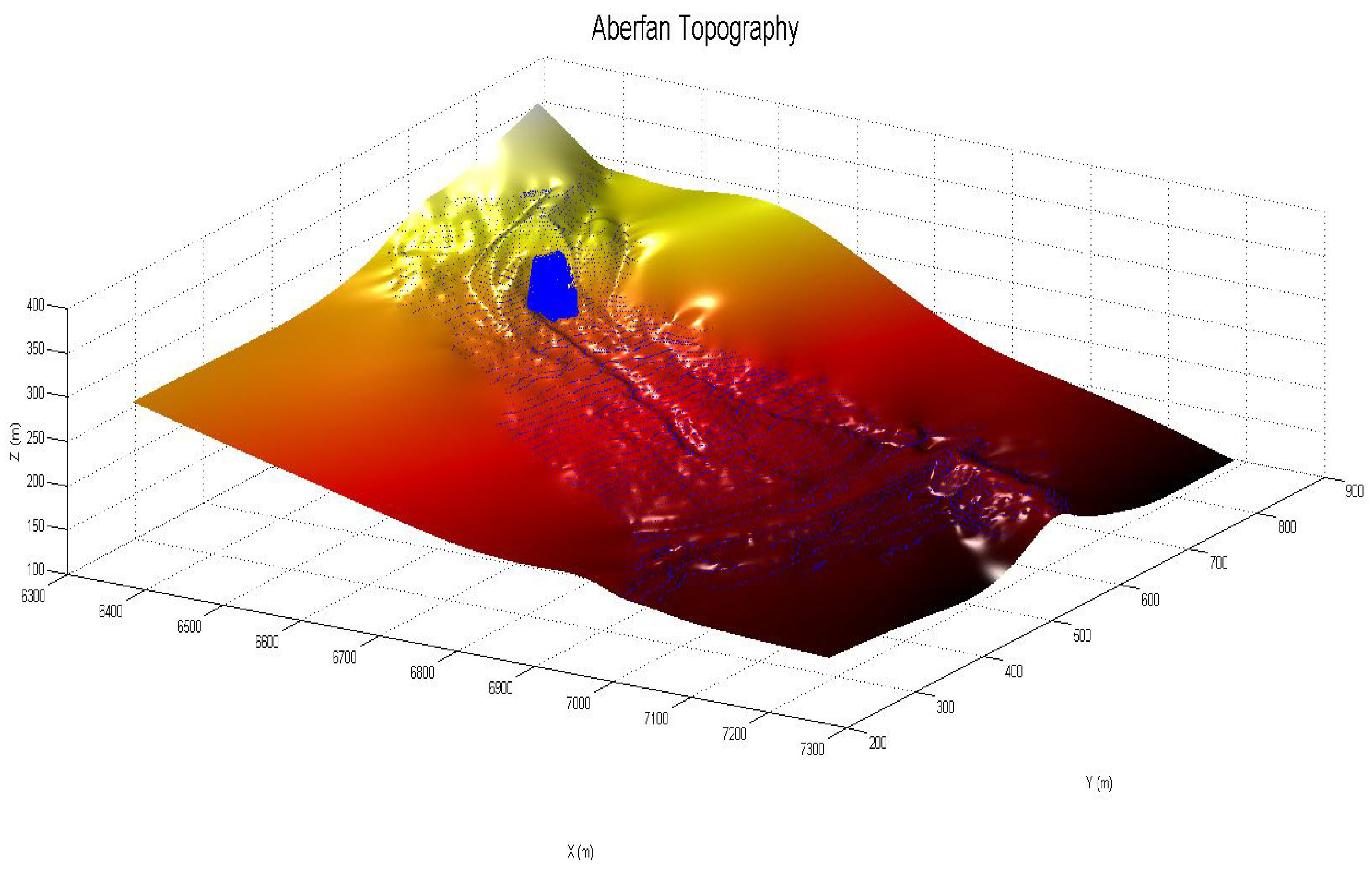
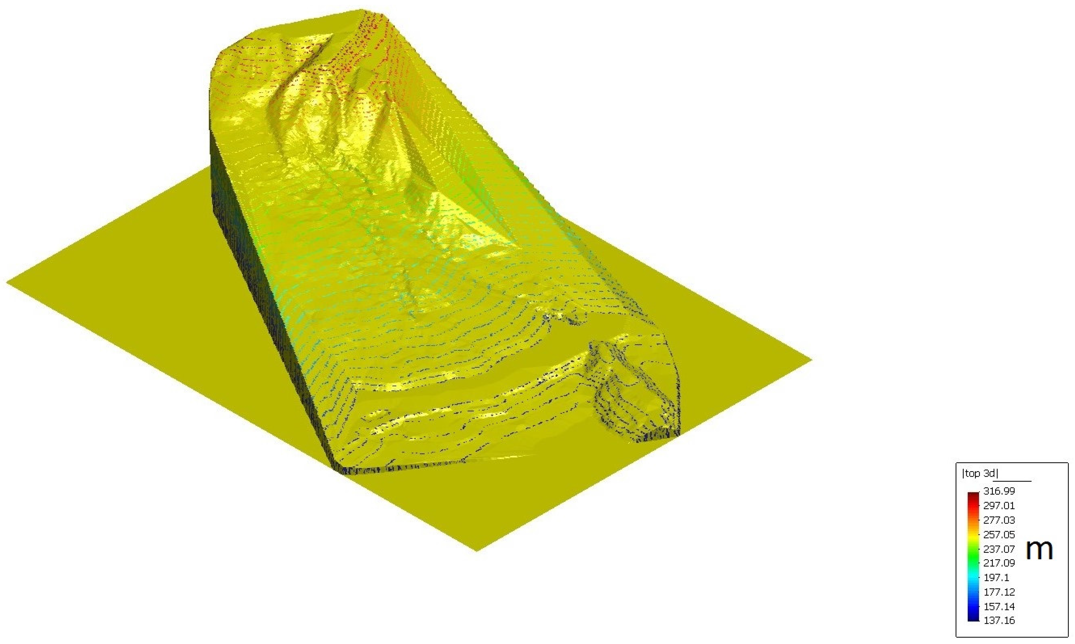
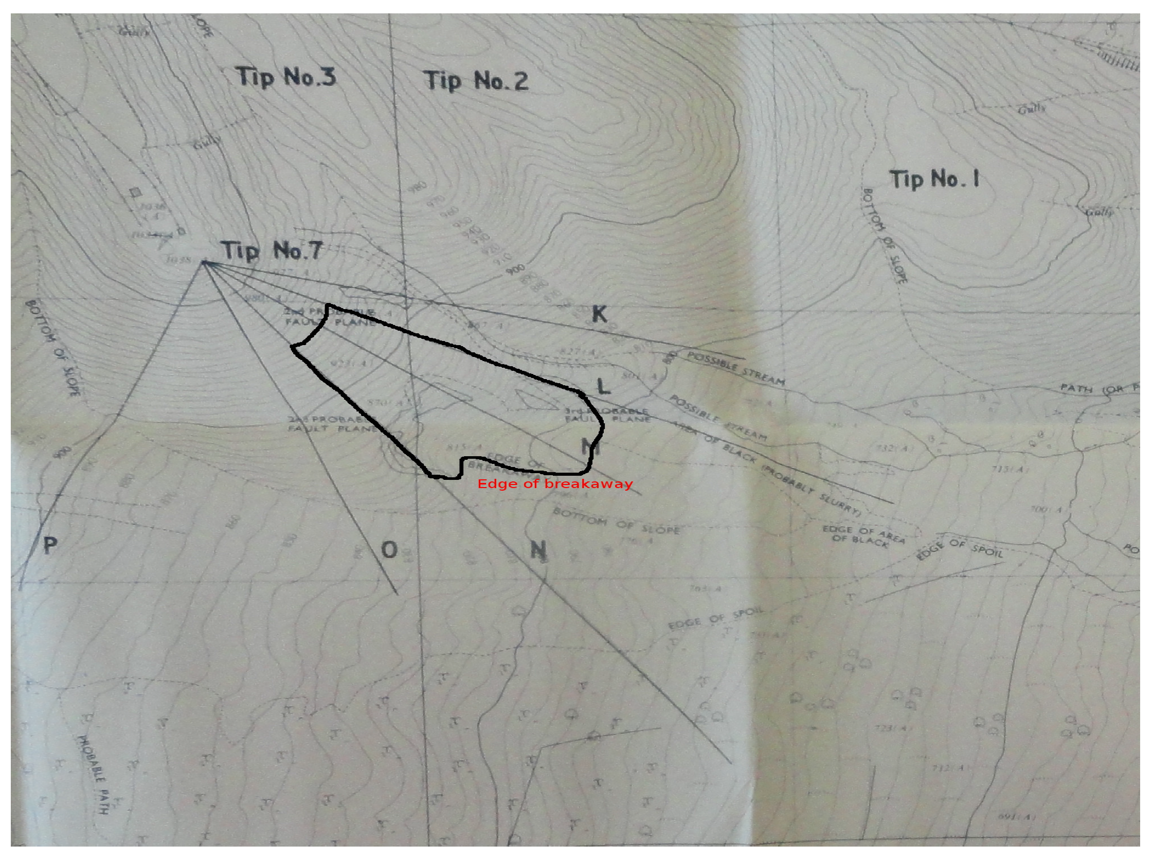
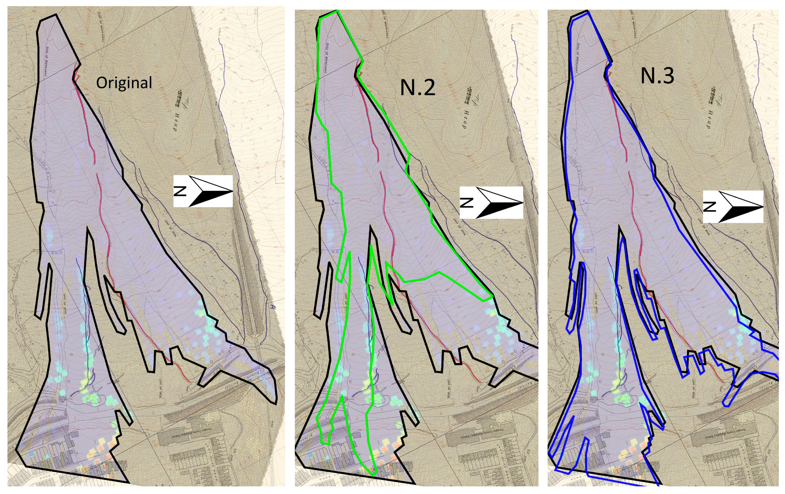
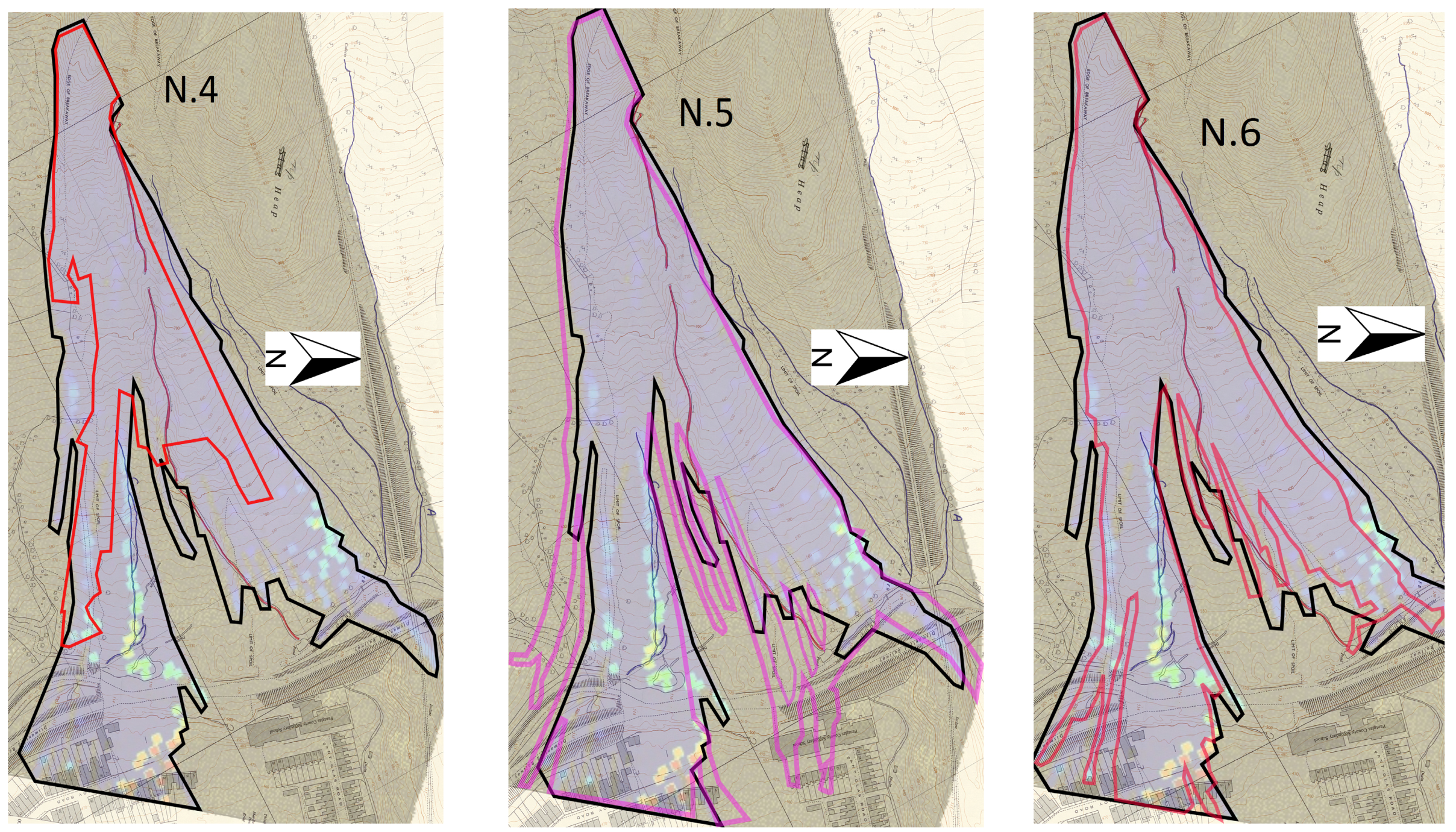
5.3. The Aberfan Flowslide
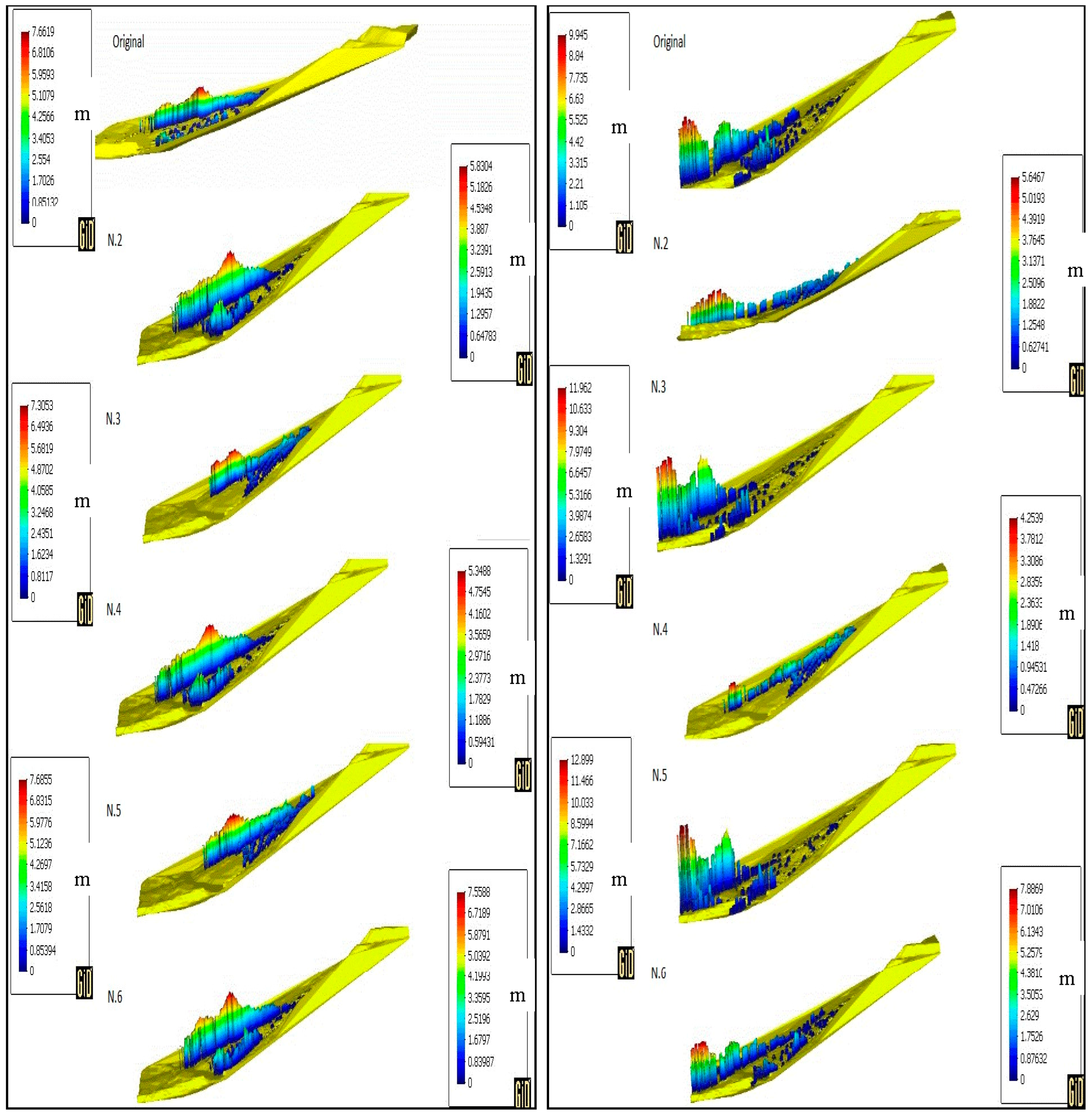
5.4. Results, Parametric Study and Discussion
5.4.1. Introduction
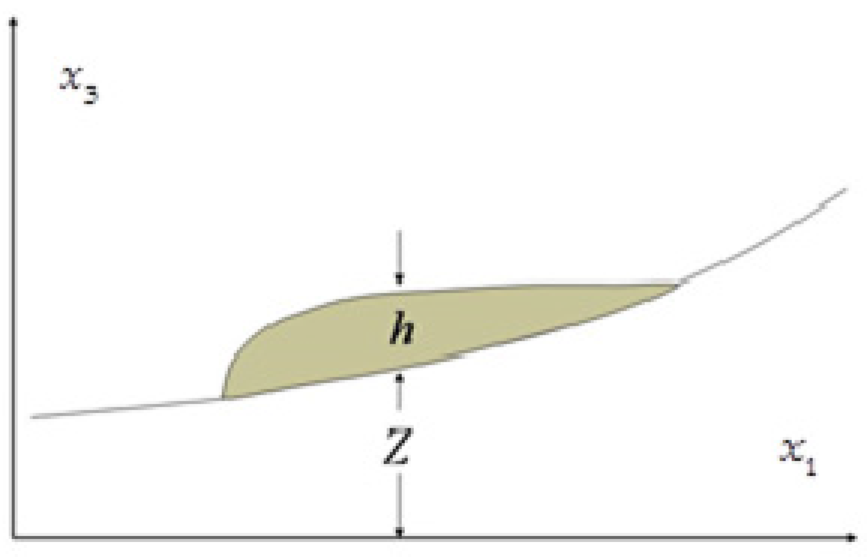
- the height of propagation
- the propagation profile
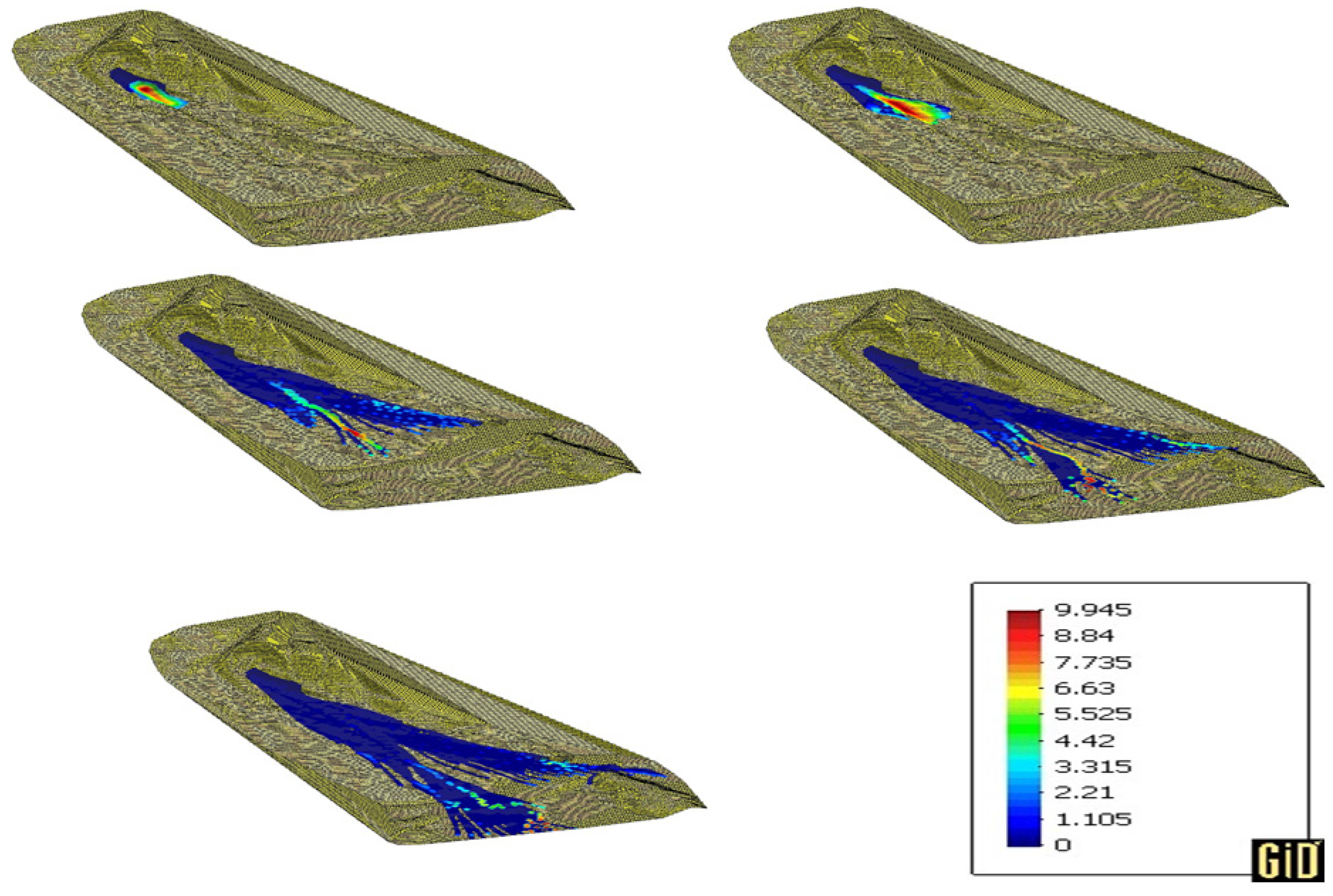
5.4.2. Simulation Results
5.4.3. Parametric Study
6. Conclusions
Acknowledgments
Author Contributions
Conflicts of Interest
References
- Savage, S.B.; Hutter, K. The dynamics of avalanches of granular materials from initiation to runout. Part I: Analysis. Acta Mech. 1991, 86, 201–223. [Google Scholar] [CrossRef]
- Iverson, R.M.; Denlinger, R.P. Flow of variably fluidized granular masses across three-dimensional terrain: 1. Coulomb mixture theory. J. Geophys. Res. 2001, 106, 537–552. [Google Scholar] [CrossRef]
- Hutter, K.; Koch, T. Motion of a Granular Avalanche in an Exponentially Curved Chute: Experiments and Theoretical Predictions. Philos. Trans. R. Soc. Math. Phys. Eng. Sci. 1991, 334, 98–138. [Google Scholar] [CrossRef]
- Naaim, M.; Vial, S.; Couture, R. St-Venant Approach for Rock Avalanches Modelling in Multiple Scale Analyses and Coupled Physical Systems. In Volume St-Venant Symposium; Presse de l’Ecole Nationale des Ponts et Chausses: Paris, France, 1997. [Google Scholar]
- Laigle, D.; Coussot, P. Numerical Modeling of Mudflows. J. Hydraul. Eng. 1997, 123, 617–623. [Google Scholar] [CrossRef]
- Pitman, E.B.; Le, L. A two-fluid model for avalanche and debris flows. Philos. Trans. R. Soc. Math. Phys. Eng. Sci. 2005, 363, 1573–1601. [Google Scholar] [CrossRef] [PubMed]
- McDougall, S.; Hungr, O. A model for the analysis of rapid landslide motion across three-dimensional terrain. Can. Geotech. J. 2004, 41, 1084–1097. [Google Scholar] [CrossRef]
- Rodriguez-Paz, M.; Bonet, J. A corrected smooth particle hydrodynamics formulation of the shallow-water equations. Comput. Struct. 2005, 83, 1396–1410. [Google Scholar] [CrossRef]
- Mangeney-Castelnau, A.; Vilotte, J.P.; Bristeau, O.; Perthame, B.; Bouchut, F.; Simeoni, C.; Yerneni, S. Numerical modeling of avalanches based on Saint Venant equations using a kinetic scheme. J. Geophys. Res. 2003, 108, 2527. [Google Scholar] [CrossRef]
- Lajeunesse, E.; Mangeney-Castelnau, A.; Vilotte, J.P. Spreading of a granular mass on a horizontal plane. Phys. Fluids 2004, 16, 2371–2381. [Google Scholar] [CrossRef]
- Pastor, M.; Blanc, T.; Pastor, M.J. A depth-integrated viscoplastic model for dilatant saturated cohesive-frictional fluidized mixtures: Application to fast catastrophic landslides. J. Non-Newton. Fluid Mech. 2009, 158, 142–153. [Google Scholar] [CrossRef]
- Pastor, M.; Quecedo, M.; Merodo, J.A.F.; Herreros, M.I.; Gonzalez, E.; Mira, P. Modelling tailings dams and mine waste dumps failures. Géotechnique 2002, 52, 579–591. [Google Scholar] [CrossRef]
- Pastor, M.; Haddad, B.; Sorbino, G.; Cuomo, S.; Drempetic, V. A depth-integrated, coupled SPH model for flow-like landslides and related phenomena. Int. J. Numer. Anal. Methods Geomech. 2009, 33, 143–172. [Google Scholar] [CrossRef]
- Hutchinson, J.N. A sliding–consolidation model for flow slides. Can. Geotech. J. 1986, 23, 115–126. [Google Scholar] [CrossRef]
- Pastor, M.; Quecedo, M.; González, E.; Herreros, M.I.; Merodo, J.A.F.; Mira, P. Simple Approximation to Bottom Friction for Bingham Fluid Depth Integrated Models. J. Hydraul. Eng. 2004, 130, 149–155. [Google Scholar] [CrossRef]
- Quecedo, M.; Pastor, M.; Herreros, M.I.; Merodo, J.A.F. Numerical modelling of the propagation of fast landslides using the finite element method. Int. J. Numer. Methods Eng. 2004, 59, 755–794. [Google Scholar] [CrossRef]
- Desai, C.S.; Siriwardane, H.J. Constitutive Laws for Engineering Materials with Emphasis on Geological Materials; Prentice Hall: Upper Saddle River, New Jersey, USA, 1984. [Google Scholar]
- Cambou, B.; di Prisco, C. Constitutive Modelling of Geomaterials; Horizon Scientific Press: Poole, UK, 2000. [Google Scholar]
- Kolymbas, D. Modern Approaches to Plasticity; Elsevier: Amsterdam, The Netherlands, 1993. [Google Scholar]
- Zienkiewicz, O.C.; Chan, A.H.C.; Pastor, M.; Paul, D.K.; Shiomi, T. Static and Dynamic Behaviour of Soils: A Rational Approach to Quantitative Solutions. I. Fully Saturated Problems. Proc. R. Soc. Math. Phys. Eng. Sci. 1990, 429, 285–309. [Google Scholar] [CrossRef]
- Hohenemser, K.; Prager, W. Über die Ansätze der Mechanik isotroper Kontinua. Zeitschrift für Angewandte Mathematik und Mechanik 1932, 12, 216–226. [Google Scholar] [CrossRef]
- Oldroyd, J.G.; Wilson, A.H. A rational formulation of the equations of plastic flow for a Bingham solid. Math. Proc. Camb. Philos. Soc. 1947, 43, 100–105. [Google Scholar] [CrossRef]
- Coussot, P.; Piau, J.M. On the behavior of fine mud suspensions. Rheol. Acta 1994, 33, 175–184. [Google Scholar] [CrossRef]
- Coussot, P. Steady, laminar, flow of concentrated mud suspensions in open channel. J. Hydraul. Res. 1994, 32, 535–559. [Google Scholar] [CrossRef]
- Coussot, P. Rheometry of Pastes, Suspensions and Granular Matter; John Wiley and Sons Inc.: Somerset, NJ, USA, 2005. [Google Scholar]
- Dent, J.D.; Lang, T.E. A biviscous modified bingham model of snow avalanche in motion. Ann. Glaciol. 1983, 4, 42–46. [Google Scholar] [CrossRef]
- Locat, J.; Demers, D. Viscosity, yield stress, remolded strength, and liquidity index relationships for sensitive clays. Can. Geotech. J. 1988, 25, 799–806. [Google Scholar] [CrossRef]
- Pastor, M.; Stickle, M.M.; Dutto, P.; Mira, P.; Merodo, J.A.F.; Blanc, T.; Sancho, S.; Benítez, A.S. A viscoplastic approach to the behaviour of fluidized geomaterials with application to fast landslides. Contin. Mech. Thermodyn. 2015, 27, 21–47. [Google Scholar] [CrossRef]
- Pastor, M.; Merodo, J.A.F.; Herreros, M.I.; Mira, P.; González, E.; Haddad, B.; Quecedo, M.; Tonni, L.; Drempetic, V. Mathematical, Constitutive and Numerical Modelling of Catastrophic Landslides and Related Phenomena. Rock Mech. Rock Eng. 2008, 41, 85–132. [Google Scholar] [CrossRef]
- Pastor, M.; Blanc, T.; Haddad, B.; Drempetic, V.; Morles, M.S.; Dutto, P.; Stickle, M.M.; Mira, P.; Merodo, J.A.F. Depth Averaged Models for Fast Landslide Propagation: Mathematical, Rheological and Numerical Aspects. Arch. Comput. Methods Eng. 2015, 22, 67–104. [Google Scholar] [CrossRef]
- Bingham, E.C. Fluidity and Plasticity; McGraw-Hill: New York, NY, USA, 1922. [Google Scholar]
- Zienkiewicz, O.C.; Cormeau, I.C. Visco-plasticity—Plasticity and creep in elastic solids—A unified numerical solution approach. Int. J. Numer. Methods Eng. 1974, 8, 821–845. [Google Scholar] [CrossRef]
- Adachi, T.; Oka, F. Constitutive equations for normally consolidated clays based on elasto viscoplasticity. Soils Found. 1982, 22, 57–70. [Google Scholar] [CrossRef]
- Desai, C.S.; Zhang, D. Viscoplastic model for geologic materials with generalized flow rule. Int. J. Numer. Anal. Methods Geomech. 1987, 11, 603–620. [Google Scholar] [CrossRef]
- Vulliet, L.; Hutter, K. Continuum model for natural slopes in slow movement. Géotechnique 1988, 38, 199–217. [Google Scholar] [CrossRef]
- Ledesma, A.; Olivella, S. Creep of slopes controlled by rainfall: Coupling viscoplasticity and unsaturated soil behaviour. In Proceedings of the 1st International Workshop on New Frontiers in Computational Geotechnics (IWS), Banff, AB, Canada, 14–15 September 2002; pp. 91–98. [Google Scholar]
- Perzyna, P. The constitutive equations for rate sensitive plastic materials. Q. Appl. Math. 1963, 20, 321–332. [Google Scholar] [CrossRef]
- Perzyna, P. Fundamental problems in viscoplasticity. Adv. Appl. Mech. 1966, 9, 243–377. [Google Scholar]
- Lucy, L.B. Numerical Approach to Testing of Fission Hypothesis. Astron. J. 1977, 82, 1013–1024. [Google Scholar] [CrossRef]
- Gingold, R.A.; Monaghan, J.J. Smoothed Particle Hydrodynamics—Theory and Application to Non-Spherical Stars. Mon. Not. R. Astron. Soc. 1977, 181, 375–389. [Google Scholar] [CrossRef]
- Pastor, M.; Manzanal, D.; Merodo, J.A.F.; Mira, P.; Blanc, T.; Drempetic, V.; Pastor, M.J.; Haddad, B.; Sánchez, M. From solids to fluidized soils: Diffuse failure mechanisms in geostructures with applications to fast catastrophic landslides. Granul. Matter 2010, 12, 211–228. [Google Scholar] [CrossRef]
- Jeyapalan, J.K.; Duncan, J.M.; Seed, H.B. Investigation of Flow Failures of Tailings Dams. J. Geotech. Eng. 1983, 109, 172–189. [Google Scholar] [CrossRef]
- Bishop, A.W.; Hutchinson, J.N.; Penman, A.D.M.; Evans, H.E. Geotechnical investigations into the causes and circumstances of the disaster of 21 October 1966. In A Selection of Technical Reports Submitted ot the Aberfan Tribunal; Her Majesty’s Stationary Office: London, UK, 1969. [Google Scholar]
- Bishop, A.W. The stability of tips and spoil heaps. Q. J. Eng. Geol. Hydrogeol. 1973, 6, 335–376. [Google Scholar] [CrossRef]
- Hungr, O. A model for the runout analysis of rapid slides, debris flows and avalanches. Can. Geotech. J. 1995, 32, 610–623. [Google Scholar] [CrossRef]


| Concept | Value | Meaning |
|---|---|---|
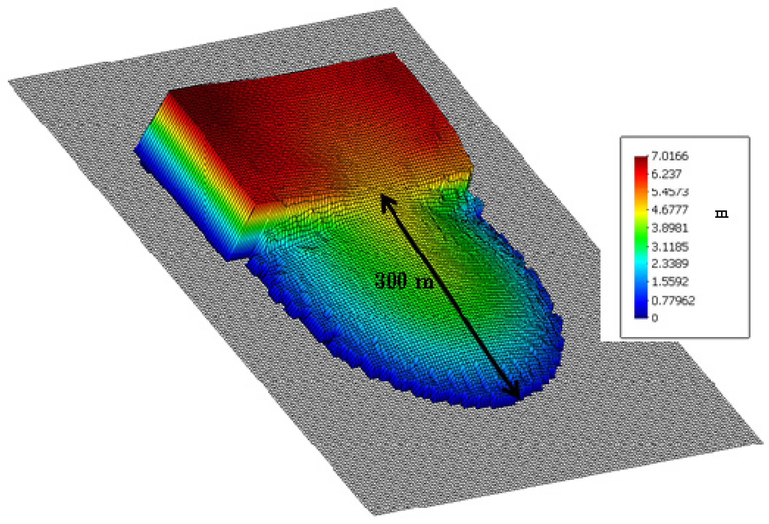
| Height | 67 m | Height measured from the toe of the slope |
| Slope Terrain | 12 degrees | Slope of the underlying terrain |
| Distance | 275 m | Distance before division into two lobes |
| Total distance | 600 m | Longest distance travelled |
| Distance to building | 450 m | Distance before the flowslide hits the first Aberfan building |
| Velocity | Estimated velocity of the flowslide |
| Parameter | Value | Meaning |
|---|---|---|
| 0.726 | Tangent of the friction angle | |
| N | 1 | Perzyna model parameter |
| 0.001 s−1 | Fluidity parameter | |
| 1740 kg·m−3 | Material density | |
| 65 × 10−4 m/s | Erosion coefficient | |
| 65 × 10−5 m2/s | Consolidation coefficient | |
| 0.8 | Initial pore pressure (relative to liquefaction) | |
| 0.4 | Initial height of basal saturated layer (relative to h) |
| Simulation | tanϕ | N | Erosion (m/s) | Viscosity (s) |
|---|---|---|---|---|
| Original | 0.726 (36°) | 1 | 65 × 10−4 | 0.001 |
| N.2 | 0.726 | 1 | 65 × 10−4 | 0.1 |
| N.3 | 0.726 | 1 | 65 × 10−4 | 0.00001 |
| N.4 | 0.726 | 1 | 0 | 0.001 |
| N.5 | 0.577 (30°) | 1 | 65 × 10−4 | 0.001 |
| N.6 | 0.839 (40°) | 1 | 65 × 10−4 | 0.001 |
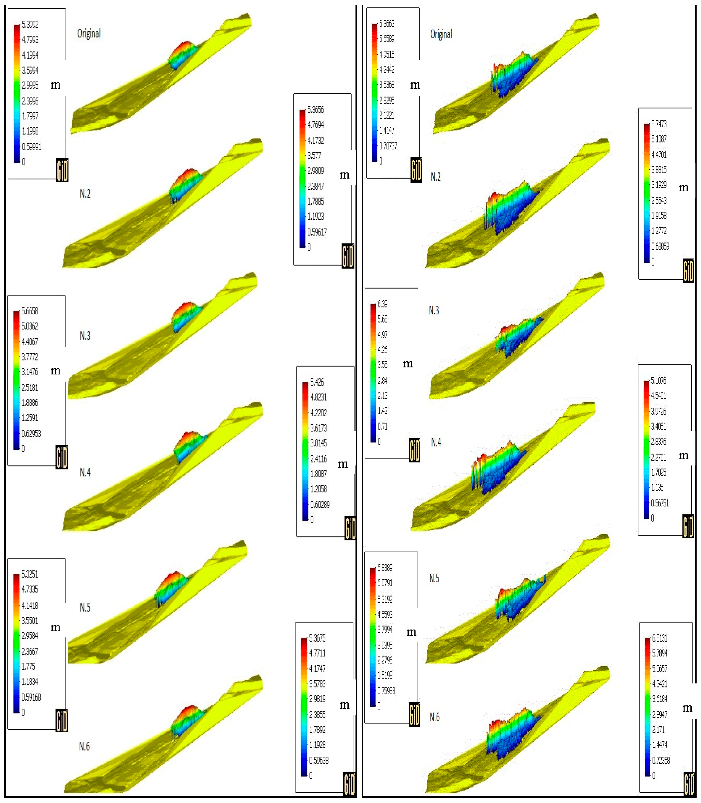
| Max Height (m) | ||||
|---|---|---|---|---|
| 10 s | 20 s | 30 s | 50 s | |
| Original | 5.3992 | 6.3663 | 7.6619 | 9.945 |
| N.2 | 5.3656 | 5.7473 | 5.8304 | 5.6467 |
| N.3 | 5.6658 | 6.39 | 7.3053 | 11.962 |
| N.4 | 5.426 | 5.1076 | 5.3488 | 4.2539 |
| N.5 | 5.3251 | 6.8389 | 7.6855 | 12.899 |
| N.6 | 5.3675 | 6.5131 | 7.5588 | 7.8869 |
© 2017 by the authors. Licensee MDPI, Basel, Switzerland. This article is an open access article distributed under the terms and conditions of the Creative Commons Attribution (CC BY) license (http://creativecommons.org/licenses/by/4.0/).
Share and Cite
Dutto, P.; Stickle, M.M.; Pastor, M.; Manzanal, D.; Yague, A.; Moussavi Tayyebi, S.; Lin, C.; Elizalde, M.D. Modelling of Fluidised Geomaterials: The Case of the Aberfan and the Gypsum Tailings Impoundment Flowslides. Materials 2017, 10, 562. https://doi.org/10.3390/ma10050562
Dutto P, Stickle MM, Pastor M, Manzanal D, Yague A, Moussavi Tayyebi S, Lin C, Elizalde MD. Modelling of Fluidised Geomaterials: The Case of the Aberfan and the Gypsum Tailings Impoundment Flowslides. Materials. 2017; 10(5):562. https://doi.org/10.3390/ma10050562
Chicago/Turabian StyleDutto, Paola, Miguel Martin Stickle, Manuel Pastor, Diego Manzanal, Angel Yague, Saeid Moussavi Tayyebi, Chuan Lin, and Maria Dolores Elizalde. 2017. "Modelling of Fluidised Geomaterials: The Case of the Aberfan and the Gypsum Tailings Impoundment Flowslides" Materials 10, no. 5: 562. https://doi.org/10.3390/ma10050562