Wave Electromechanical Coupling Factor for the Guided Waves in Piezoelectric Composites


1
School of Energy and Power Engineering, Beihang University, Beijing 100191, China
2
Beijing Key Laboratory of Aero-Engine Structure and Strength, Beijing 100191, China
3
Laboratoire de Tribologie et Dynamique des Systemes, Ecole Centrale de Lyon, 69130 Ecully, France
*
Author to whom correspondence should be addressed.
Materials 2018, 11(8), 1406; https://doi.org/10.3390/ma11081406
Submission received: 21 July 2018
/
Revised: 2 August 2018
/
Accepted: 6 August 2018
/
Published: 11 August 2018
(This article belongs to the Section Smart Materials)
Abstract
:A novel metrics termed the ‘wave electromechanical coupling factor’ (WEMCF) is proposed in this paper, to quantify the coupling strength between the mechanical and electric fields during the passage of a wave in piezoelectric composites. Two definitions of WEMCF are proposed, leading to a frequency formula and two energy formulas for the calculation of such a factor. The frequency formula is naturally consistent with the conventional modal electromechanical coupling factor (MEMCF) but the implementation is difficult. The energy formulas do not need the complicated wave matching required in the frequency formula, therefore are suitable for computing. We demonstrated that the WEMCF based on the energy formula is consistent with the MEMCF, provided that an appropriate indicator is chosen for the electric energy. In this way, both the theoretical closure and the computational feasibility are achieved. A numerical tool based on the wave and finite element method (WFEM) is developed to implement the energy formulas, and it allows the calculation of WEMCF for complex one-dimensional piezoelectric composites. A reduced model is proposed to accelerate the computing of the wave modes and the energies. The analytical findings and the reduced model are numerically validated against two piezoelectric composites with different complexity. Eventually an application is given, concerning the use of the shunted piezoelectric composite for vibration isolation. A strong correlation among the WEMCF, the geometric parameters and the energy transmission loss are observed. These results confirm that the proposed WEMCF captures the physics of the electromechanical coupling phenomenon associated with the guided waves, and can be used to understand, evaluate and design the piezoelectric composites for a variety of applications.
1. Introduction
The concept of smart structures provides another promising possibility of solving a variety of engineering issues, such as vibration control, noise reduction, fault diagnose, wireless sensing, self powering and so on. Smart structures could be defined as ‘the structures that can sense external disturbance and respond to that in a desired fashion’ [1]. Generally a smart structure can be implemented by integrating some ‘smart materials’ that couple at least another field to the mechanical field. This introduces new design variables to modify or measure the mechanical characteristics. An additional subsystem can then be designed regarding the new variables so as to have the coupled structural system work in a desired manner. These smart materials involve electrorheological (ER) materials, magnetorheological (MR) materials, magnetostrictive materials, electrostrictive materials, shape memory alloys (SMA), piezoelectric materials and so on. Among them all, the piezoelectric materials have the advantages of light-weight, large working frequency range and high power density, therefore they are undoubtedly the most mature and those with the most applications [2].
Piezoelectric effect that couples the electric and mechanical fields is the corner stone of all the piezoelectric-based smart structures. It naturally comes into a question that how to quantitatively describe the ’strength’ of the electromechanical coupling induced by the piezoelectric materials. The criteria that can measure the converting capability or the coupling strength are termed the ‘electromechanical coupling factors’ (EMCF). In general, there are two scales regarding EMCF. The first one is the material scale [3]. EMCF in this scale is used to describe the coupling strength or converting capability of a piezoelectric material under certain uniaxial stress situations. EMCF in this scale is therefore directly related to the material parameters. For instance for the thickness stretch deformation (referred to as the ‘13’ mode), the coupling factor , where , and are all material parameters [4]. Likewise, terms , can also be obtained for the longitudinal (the ‘33’ mode) and torsional (the ‘51’ mode) deformation respectively. These terms are also called static coupling factors. They allow one to choose an appropriate piezoelectric material before it is manufactured into certain components. They are especially useful in actuating and sensing [5,6] where a uniaxial tress field is assumed.
If we consider the host structure and the piezoelectric materials/transducers as a whole, and concern the dynamic behaviour, the EMCF should be defined in the structural scale. A widely recognized approach is to define the EMCF based on natural modes [4,7], by
where and are the resonance and anti-resonance frequencies in the frequency response fuction (FRF) of respectively; V and Q are the voltage and charge of the piezoelectric materials respectively. Moreover, is also the open-circuit frequency of a mode and is also the short-circuit modal frequency [8]. Term is therefore called modal electromechanical coupling factor (MEMCF) [9] as well. Theoretically speaking, arbitrary deformation of a finite structure can be expressed as the superposition of the modal deformations, and the modes whose natural frequencies are close to the considered excitation frequency range will have dominant contribution. In this regard, it is reasonable to define the EMCF in terms of modes. Please obtaining the MEMCF is very convenient both experimentally and numerically because only two set of modal analysis results are required. MEMCF as a metrics in the structural scale has many important applications. A direct application is the design of modal transducers [8,10], where the MEMCF is used to examine whether the piezoelectric subsystem is coupled only with the target mode (modal sensor) or it is uncoupled with the target mode(modal filter). Another application is the passive vibration control. Thomas et al. [9] found, via closed-form expressions, that the best modal damping induced by the resistor and resistor-inductor shunts depend only on the MEMCF once the structural parameters remain constant. This indicates that MEMCF can be used as a criterion to optimize the geometrics of the piezoelectric materials [11,12].
Alternatively, the structural deformation can also be described by the superposition of wave motions, while natural modes are understood as standing waves induced by the reflection of waves on the boundaries [13,14,15]. The wave perception is especially suitable in dealing with high-frequency or transient vibration problems, where many modes are involved and the resonance behaviour is less apparent. Many piezoelectric strategies have been proposed based on the wave perception. For example, the periodically distributed piezoelectric materials with identical shunting circuits are used to modify the wave properties in the interested frequency band so as to dissipate or localize the injected energy [16,17,18,19]. Moreover, piezoelectric materials are designed as actuators and sensors for the waves in cylinders [20,21] and plates [22,23,24] for structural health monitoring (SHM) purpose.
In the wave perception, the EMCF should quantify the coupling strength between the mechanical and electric fields during the passage of a wave in piezoelectric composites, and in this paper it is termed the ‘wave electromechanical coupling factor’ (WEMCF) to distinguish itself from the aforementioned coupling factors. Only a few works have been devoted to this subject, and WEMCF is defined by different means. Chen et al. [25] calculated WEMCF by for Rayleigh-type surface acoustic waves in a semi-infinite with alternating piezoelectric and non-piezoelectric super-lattices, where and are the group velocity in open-circuit and short-circuit situation respectively. Fan et al. [26] used the Green’s function method to calculate the WEMCF for a Lamb wave in a multi-layered plate. The authors [27] defined the WEMCF as the proportion of the electric energy associated with the block capacitance in elastic energy. We showed that the WEMCF can be used to decouple the geometric design from the electric design for the one-dimensional piezoelectric waveguide, and it allows to achieve the desired band gaps by using a minimum amount of piezoelectric materials.
The existing studies of WEMCF raise two questions: (1) Is the proposed WEMCF consistent with the MEMCF? and (2) How to build a general numerical tool for the calculation of WEMCF for complex piezoelectric composites? Since a structural dynamics problem is always possible, at least in principle, to arrive at the same conclusions by either mode or wave approach (often referred to as ‘wave-mode duality’ [14,15]), a positive answer should be given of the first question to achieve theoretical closure. The second question should be addressed so that WEMCF can be used in real engineering applications.
In this paper, we further study the WEMCF for one-dimensional piezoelectric waveguide and address both the aforementioned questions. In Section 2 we propose a frequency formula to define the WEMCF. It is difficult to implement but it is naturally consistent with the MEMCF. Then we propose two energy formulas to approximate the frequency formula. Since the energy formulas are easier to implement, both the theoretical closure and the computational feasibility are achieved. To do that, we first outline the wave and finite element method (WFEM) in Section 3, including the basic procedures and a reduced model applicable for piezoelectric composites. In Section 4 the energy formulas are discussed in detail, including the definition, demonstration and implementations. In Section 5 the analytical findings and implementations are validated. It is also shown that the use of the reduced unit cell model can rapidly and accurately capture the WEMCF. Eventually, an application concerning the control of energy flow using shunted piezoelectric composite is presented in Section 6, in order to illustrate the usage of WEMCF.
2. Definitions of WEMCF
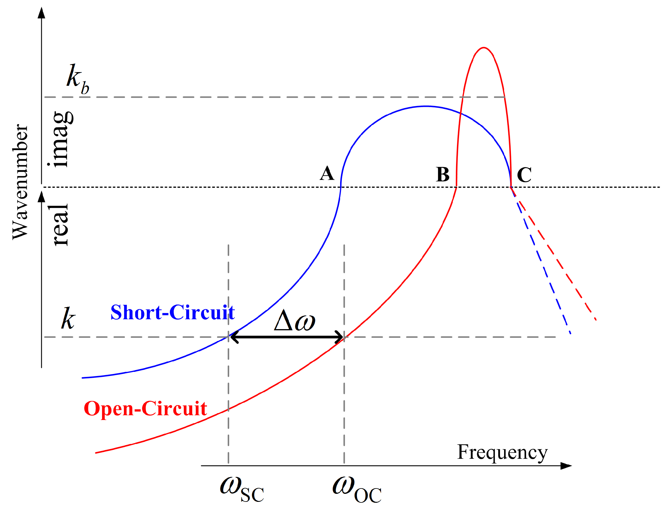
It is widely known that the equivalent stiffness of the piezoelectric materials will be changed when the electrodes are set to the short circuit (SC) or open circuit (OC) statuses. Consequently, a piezoelectric composite will exhibit different dispersion curves in SC and OC statuses [18], as illustrated in Figure 1. This inspires us to use the relative difference of the propagating frequencies of OC and SC statues to define the WEMCF , as:
where and are the propagating frequencies of the wave in the OC and SC statuses respectively. This equation is similar to Equation (1) which defines the MEMCF [4,8,28], but the frequencies terms have different physical means.
Please note that the wave shapes at the border frequencies of a band gap, namely A, B and C in Figure 1, are also the modal shapes of the piezoelectric composite under certain boundaries conditions [29]. This fact indicates that the coupling strength of these waves (A, B and C) can be given either by WEMCF or MEMCF. The WEMCF and MEMCF should give the same value at these frequencies, because a same deformation should be given a same value of its electromechanical feature, no matter the deformation is understood as a wave or a mode. In this case the travelling frequencies of the waves ( and ) are exactly the natural frequencies ( and ) of the modes. Hence Equations (1) and (2) yield the same value. This means that WEMCF defined by Equation (2) is consistence with MEMCF.
Definition of WEMCF by Equation (2) may be reasonable and intuitive. However, there are two main challenges. The first one is that Equation (2) works only for propagating waves, because band gaps may have different depth in OC and SC statuses, shown in Figure 1. Consequently it is difficult to link the evanescent waves between OC and SC, for example in Figure 1 the wave with wavenumber does not have its corresponding wave in the SC case. The second challenge is related to computational issues. For complex waveguide whose dispersion relations has veering and intersection (examples can be found in reference [30,31]), it will be difficult to correlate same type of propagating waves from the dispersion relations at OC and SC statues.
Alternatively, WEMCF can be defined by the fraction of energies at one electrode status:
where is the electric energy and V is the mechanical energy. This definition is applicable for both evanescent and propagating waves. It only requires the dispersion curves at one situation so no efforts are needed to correlate the waves between OC and SC. Wave shapes have to be known to calculate the energies and V. In the following sections we will present different ways for the calculation of the energy terms in Equation (3) based on wave and finite element method (WFEM). The consistency with MEMCF will be demonstrated and validated.
3. Wave and Finite Element Method (WFEM)
Wave and finite element method (WFEM) [30,32,33,34] is a general numerical tool widely used to analyse the free and forced wave propagation in uniform and periodic structures. It requires only the modelling of the smallest repetitive substructure (termed the unit cell) of the whole structure, therefore is much faster than the conventional finite element method. WFEM yields the dispersion curves of the waves by solving the eigenvalue problem which can be formulated in many different ways [35]. In this paper, WFEM is developed to compute the required energy terms, and also as a general representation of the dynamics of the piezoelectric composite. The properties of the wave shapes derived from WFEM will be used later to demonstrate the consistency between the WEMCF and MEMCF. For these reasons we briefly outline the basic procedure of WFEM. A reduce model for the piezoelectric composite proposed earlier by the authors [31,36] is also outlined, and it will be used to accelerate the computing the energy terms.
3.1. Basic Procedure
The first step of WFEM is to model one unit cell by finite element method. Any existing FEM package can be used, and in this paper ANSYS 17 is applied to generate the mesh and the required matrices of the unit cell modelling. All the following-up procedures of WFEM, including the solving of the eigenvalue problem, the reduced model, the post-processing are implemented by an in-house Python code developed by the authors. The Python code is validated against the analytical and full finite element method in many applications [30,31,36]. In absence of any external loads, the dynamic equations of a unit cell in the periodic piezoelectric structure write
where is the displacement vector and the force vector; and denote the generalized stiffness and mass matrices respectively; Subscripts L, R, I and E respectively refer to the left-side, right-side and internal mechanical Degree-of-freedoms (DOFs) and the electric voltage DOFs; A dot means derivation with respect to time t. The terms are also illustrated in Figure 2.
Specifically, the generalized mass matrix has the form of
and the generalized stiffness matrix writes
where and are the mechanical stiffness and piezoelectric matrices respectively, the intrinsic capacitance matrix and external electric impedance. More details about the finite element model of a piezoelectric structure can be found in Benjeddou’s review [37].
The second step of WFEM is taking into account the periodicity. According to the Bloch theory, the wave of the form that travels in the periodic structure should satisfy the condition
where describes the amplitude and phase change when the wave propagates from the left side to the right side of a unit cell. k is the wavenumber and is the length of the unit cell along the propagation (periodicity) direction. Additionally, the equilibrium between the adjacent cells implies
Then the aim of the wave modal analysis is to find associated with and k to satisfy Equations (4), (7) and (8) at the same time.
To solve these equations, we can fix , and search for k and . At angular frequency , the dynamic equation of a unit cell writes
After condensing all the internal DOFs at frequency , it gives
where
Introducing condition (7) and (8) into Equation (10), and eliminating and , it comes to the following eigenvalue problem
Eigenvalue problem (12) yields all the wavenumbers and associated deformations (termed wave shape) that can occur in the waveguide at the given frequency. Repeating the calculation in different frequencies the dispersion curves can be obtained. The required energy terms in (3) can be calculated from the wave shapes, and this will be further discussed in Section 4.1.
3.2. Reduced Model for the Piezoelectric Composites
Though WFEM is more efficient that the conventional finite element method in terms of wave-dispersion and forced response analysis at high frequencies, it also requires long computational time if the internal DOFs are enormous. The main reason is that in Equation (11), a matrix inverse is required at each frequency. The computational efficiency significantly decreases with the increase of matrix dimension. This corresponds to the situation where the waveguide has complicate configuration on each unit cell. In this paper, the computing of energies are required as shown in (3), this amplifies the computational cost. To accelerate the computing, we employ the reduce model proposed by the authors [31,36] because it is proved applicable for piezoelectric structures.
First, we define the transformation relation
where , and is the kth natural mode of the unit cell with and the corresponding natural frequencies is . Namely, and with are obtained as the eigenvectors and eigenvalues of
Only l modes are kept in , and the number is less than that of . The criterion for the selection of the retained modes is where is the maximum excitation frequency to be considered. After introducing Equation (13) into Equation (4), the dynamic equations of a unit cell become:
where
After these operations, the internal mechanical DOFs are transformed from to , and the dimension of is much smaller than . In this way, the computing of Equation (11) is accelerated. Moreover, the technique also reduces the size the of wave shape, this is especially useful for the computing of the energies as it will be shown in Section 5.
4. Energy Formulas of WEMCF
4.1. Two Energy Formulas
Suppose a propagating wave exists in the OC status with wave shape , wavenumber k and frequency . Two specific energy formulas of Equation (3) are proposed, as
and
where V is the mechanical potential energy, is the electric potential energy stored in the free intrinsic capacitance (the capacitance when imposing ) and is the electric potential energy stored in the block capacitance . These energy terms can be obtained by the waveshapes and matrices of the unit cell:
where for the simplification of equations. Both and are the approximations of based on different assumptions. The demonstrations are given as follows.
4.2. Demonstrations
4.2.1. Relationship between the Wavenumber and Wave Shape
Introducing these two transformations to Equation (4), by per-multiplying and multiplying at both sides of the equation, we have
where
This shows that the wave shape in the form of is also the eigenvector of Equation (25), and its associated eigenvalue is where is the propagating frequency of the wave at wavenumber k. In practice Equation (25) provides another mean to calculate the dispersion curves of the waves [35], sometimes termed the ‘direct form’ [38]. Here we use these equations in the demonstration as useful properties between wave modal shape and the corresponding wavenumber.
For a propagating wave, the wavenumber k is a real number therefore is a complex value with amplitude 1. Consequently in Equation (23) is the conjugate transpose of in Equation (24), namely
Introducing the OC eigenvector into Equation (25) and multiplying both sides of the equation by , it gives
and according to Equations (26)–(28), we know align* HOCKOC = HOCKOC
HOCMOC = HOCMOC leading to
This means that once the wave shape is known, we will also know the associated wavenumber. Equation (30) shows such a relation in OC status, later we will also do this in SC status. However, we will not use the ‘real’ SC wave shape to calculate SC propagating frequency but use the information in OC status to have a good guess of the SC wave shape and use it to estimate the SC propagating frequency.
4.2.2. Demonstration of Energy Formula
For SC situation, if we assume that mechanical deformation under a same wavenumber k remains the same, namely
and introduce into Equation (25) and multiplying both sides of the equation by , it gives
where is an approximated frequency for the SC case. Please note that matrix has zero terms in the lines correspond to the electric DOFs, shown in Equation (5), it makes
4.2.3. Demonstration of Energy Formula
The core of the demonstration in the previous section is to guess the SC wave shape based on the OC wave shape, and it was assumed that the mechanical deformation under a same wavenumber k remains the same in the SC and OC situations. More accurately, we can remove the static contribution of the OC voltage from the mechanical field so as to approximate the SC wave shape . Namely,
Similarly, the following statement holds
and with the fact that
we can give another approximation of , as
4.3. Implementations
We proposed three different ways to calculate WEMCF: one frequency formula (2) and two energy formulas (18) and (19). Since the WFEM can be implemented by the full or reduced models, there are even more paths to implement WEMCF, as shown in Figure 3. For the calculation of , there are two ways to calculate the required SC and OC frequencies. For the and that are based on energy terms, the wave shapes are required. To do that three paths are possible: the full shapes obtained by full WFEM which is the slowest, the full shapes obtained by reduced WFEM and the reduced shapes obtained by reduced WFEM. In combine there are 8 different ways to implement WFEM: 3 for , 3 for and another 2 for . In the next section we will examine the efficiency and accuracy of the implementations, and finally give the best path.
5. Validations
5.1. Validation of the Implementations
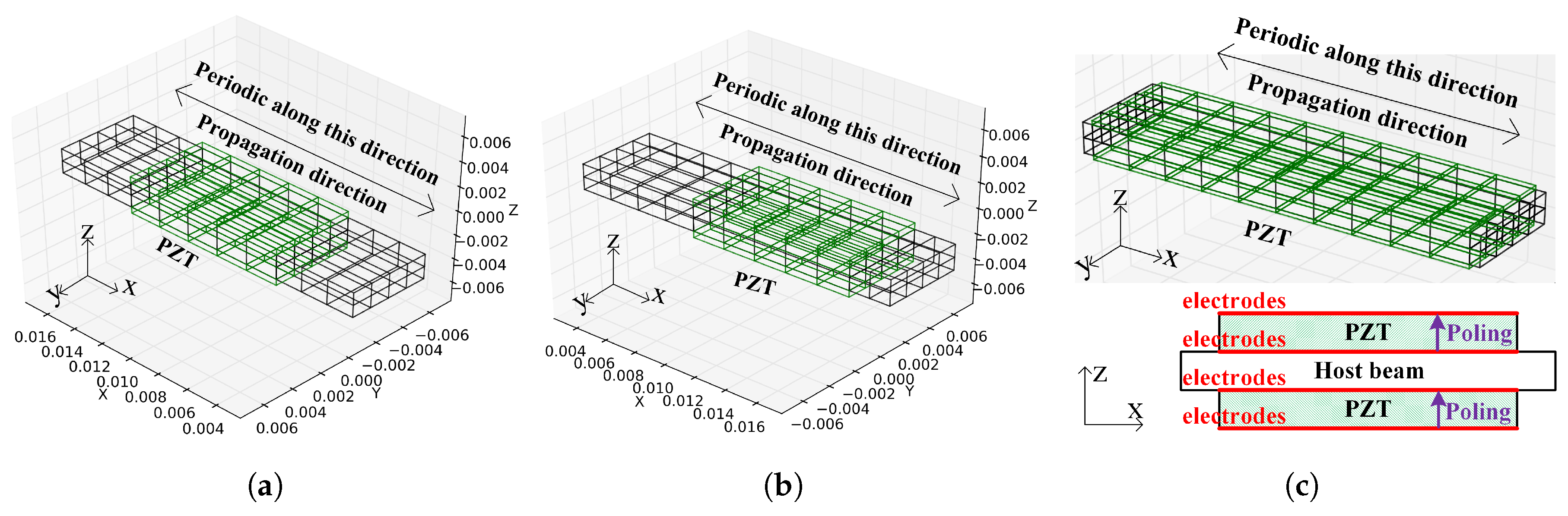
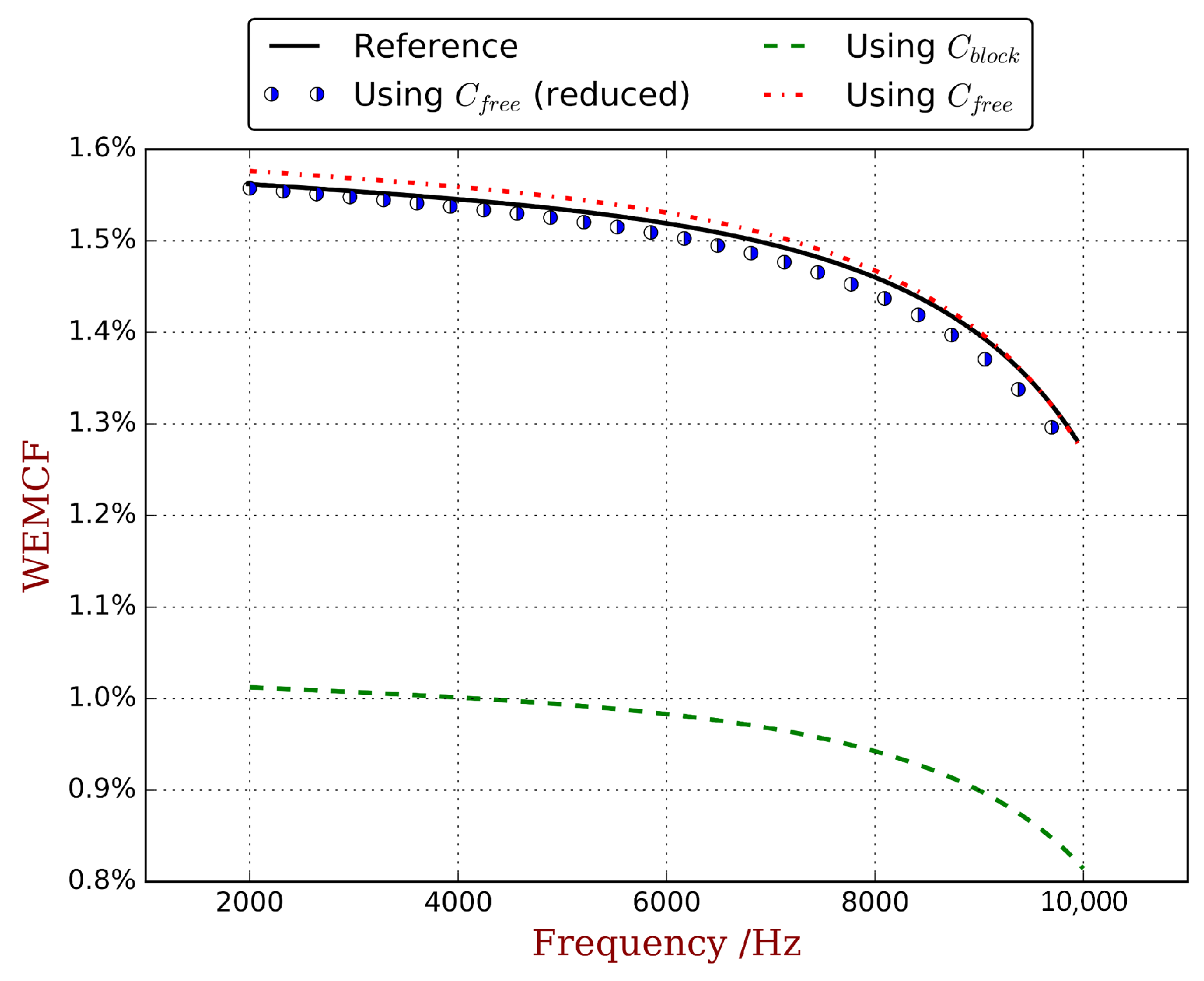
As mentioned, the consistency of WEMCF with MEMCF is strongly desired, and is consistent with MEMCF. Therefore the calculated by full WFEM is regarded as the reference. The piezoelectric waveguide with unit cell A shown in Figure 4a is considered. The mesh quality of these models are verified by the forced response analysis [31]. The host material is steel without damping, with a Young’s modulus of , a Poisson’s ratio of and a density of . The used piezoelectric material is whose material parameters are listed in the Appendix A. The WEMCF for the z-transverse wave from to is computed through all 8 paths listed in Figure 3, and the highlighted results are compared in Figure 5. The main observation is that all 3 paths for have significant errors, even though the overall tendencies are the same as the reference. The other 5 paths all return acceptable results with relative error less than 3%. This may due to the fact that assumption (38) is more precise than (31).
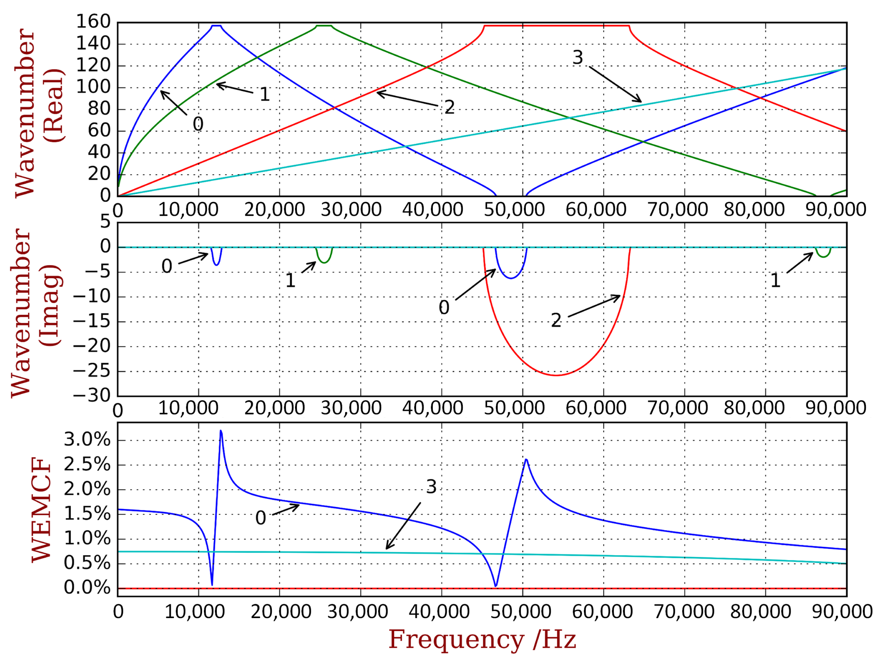
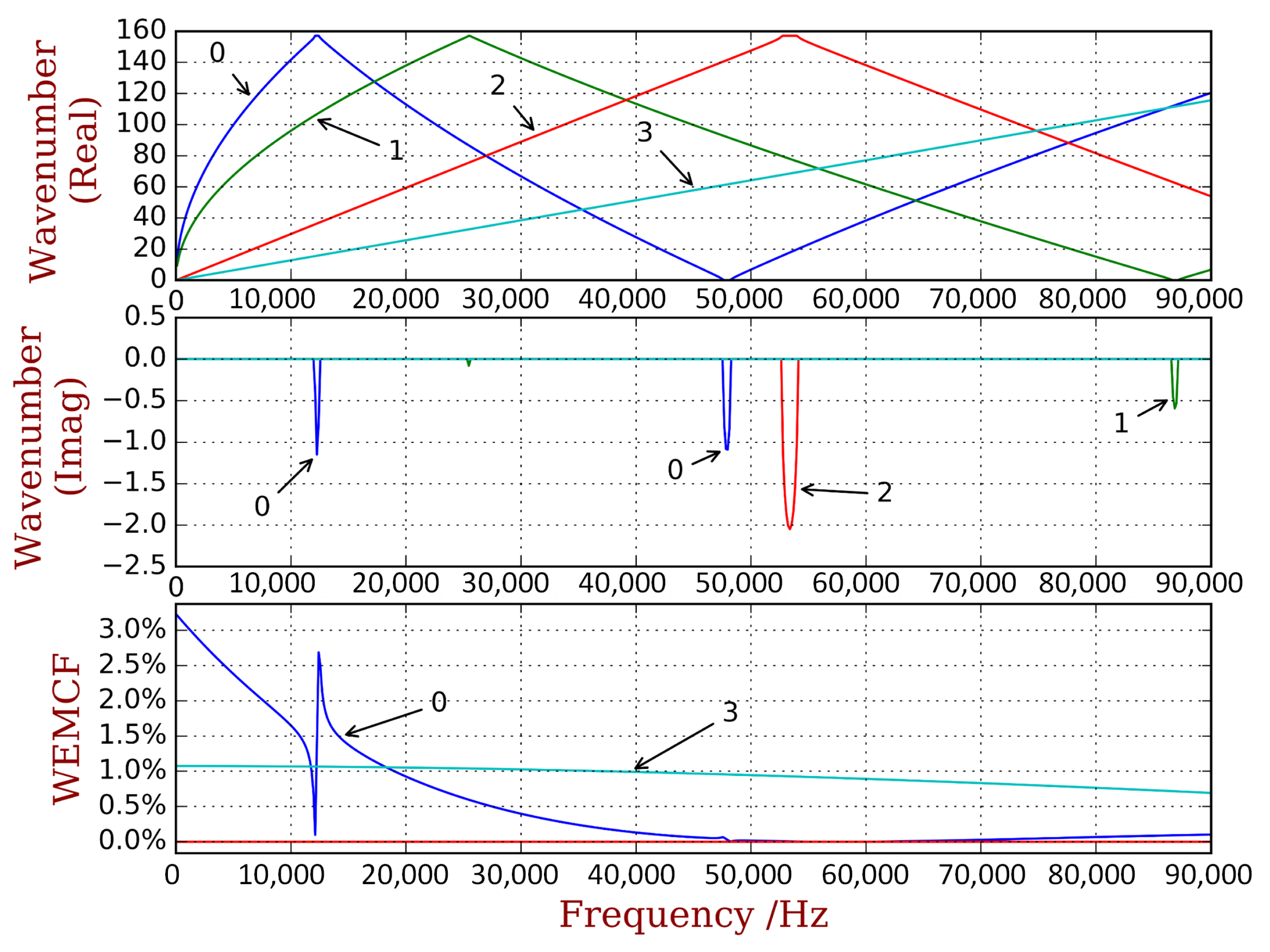
A complete dispersion curves and WEMCF results for the piezoelectric periodic structure with unit cell A is shown in Figure 6. It is shown that the z-axis flexural wave (marked by number 0) has the most significant electromechanical coupling. Weaker WEMCF is observed for the longitudinal wave (3). No coupling effects are reported for the torsional (2) and y-axis flexural waves (1). These conclusions can be acknowledged by the geometric configuration of the unit cell and engineering common sense. It is interesting to see that the largest and lowest values emerge at the border frequencies of the band gaps. The wave shapes of these waves are presented in Figure 7. The symmetric wave shapes generates different kind of charges on the electrode, cancelling each other, leading to a very low WEMCF. On the contrary, anti-symmetric shapes always generate same kind of charges hence maximize the WEMCF.
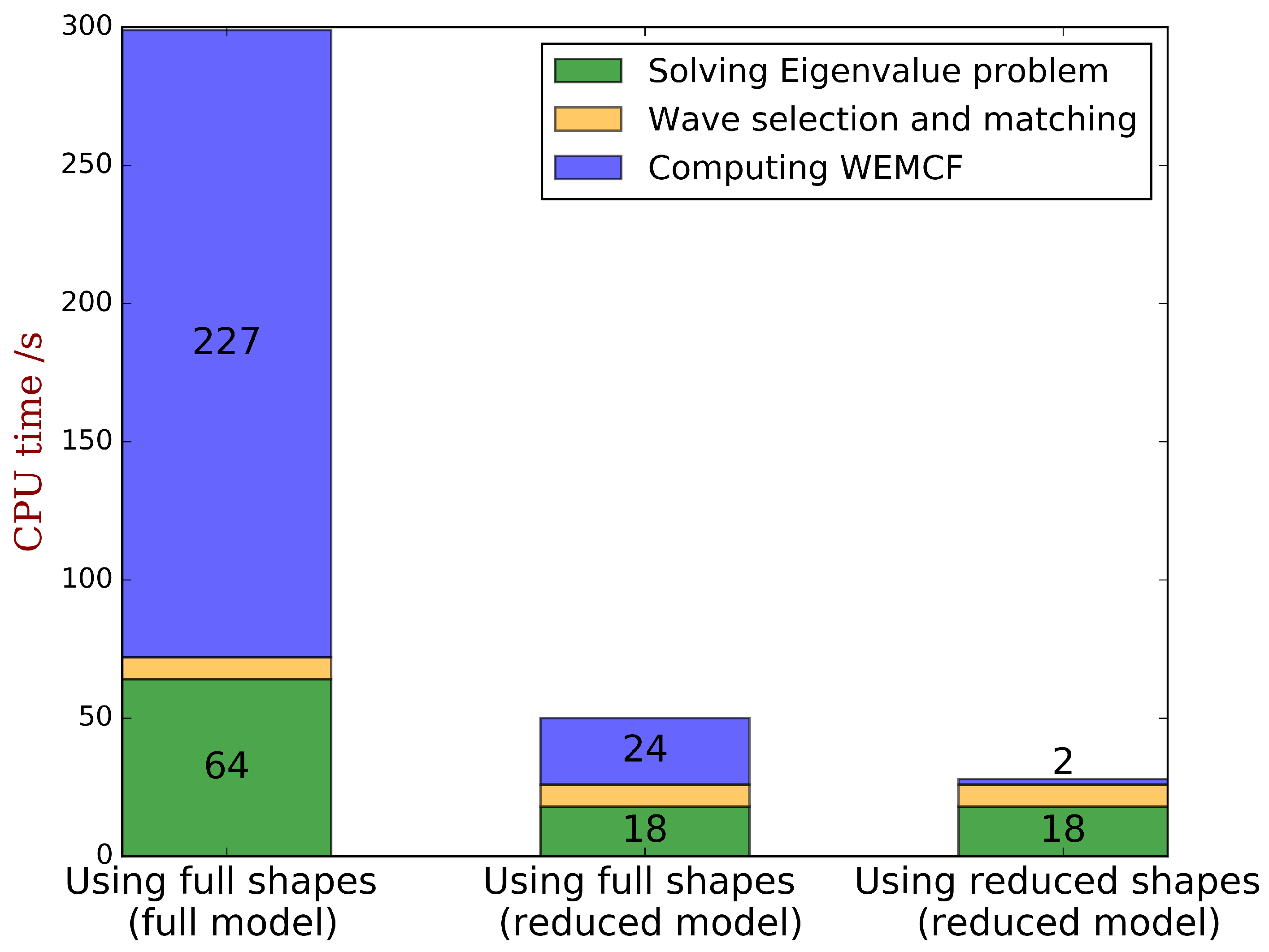
As discussed, among all the valid paths, the ones use are difficult to be programmed for general cases. There remains 3 valid paths for : (1) using full shapes obtained from the full WFEM; (2) using full shapes obtained from the reduced WFEM; (3) using the reduced wave shapes. The CPU time for obtaining the full dispersion characteristics with WFEM of unit cell A are compared in Figure 8. It shows that the post-processing for WEMCF for the full WFEM is a heavy task, and the CPU time is nearly 3 times of the free-wave analysis. While the reduced unit cell model is used, the computing time for WEMCF is reduced even when using the full wave shapes. The CPU time has the same magnitude as the free-wave analysis in this case, because the reduced model can accelerate the mapping from the cross-section DOFs to the internal DOFs by avoiding the matrix inverse. Only minor additional time is required when reduced shapes are used to compute the energy terms for WEMCF, it reduces the post-processing by in comparison to the full WFEM.
The infinite periodic structure with unit cell A can also be represented by an unsymmetrical unit cell B, shown in Figure 4b. As discussed in the literature [39], the dispersion curves should be the same as unit cell A. We also found that the WEMCF results remain the same as well. The minimal and maximal WEMCF still happen at the border frequencies of band gaps. While using the unsymmetrical unit cell, the wave shape of a unit cell is no longer symmetric, but the deformation on the PZT patches are still symmetric or anti-symmetric, leading to zero or maximum WEMCF. To make the paper more concise, the results associated with unit cell B are not presented.
Finally, we analyze the WEMCF of PZT waveguide with unit cell C, shown in Figure 4c. The unit cell has the same length as unit cell A and B but with longer PZT patches. The results are shown in Figure 9, where we observe a better WEMCF in lower frequencies than higher ones. This can be explained by checking the wave shapes shown in Figure 10. It can be seen that in higher frequencies the charges generated by the deformation will start to cancel each other. The comparison between unit cell A and C also acknowledges the engineering common sense that long PZT path works poorly in high frequencies.
5.2. Validation against a Thin-Wall Piezoelectric Structure
In the previous sections, we show that is a proper way to define the WEMCF because it is a good approximation of the which is consistent with MEMCF. Using the reduced wave shape associated with the reduced model in WFEM to compute the required energies is a very efficient implementation towards , as marked in Figure 3. In this section, we use a more complex piezoelectric structure to further examine such findings.
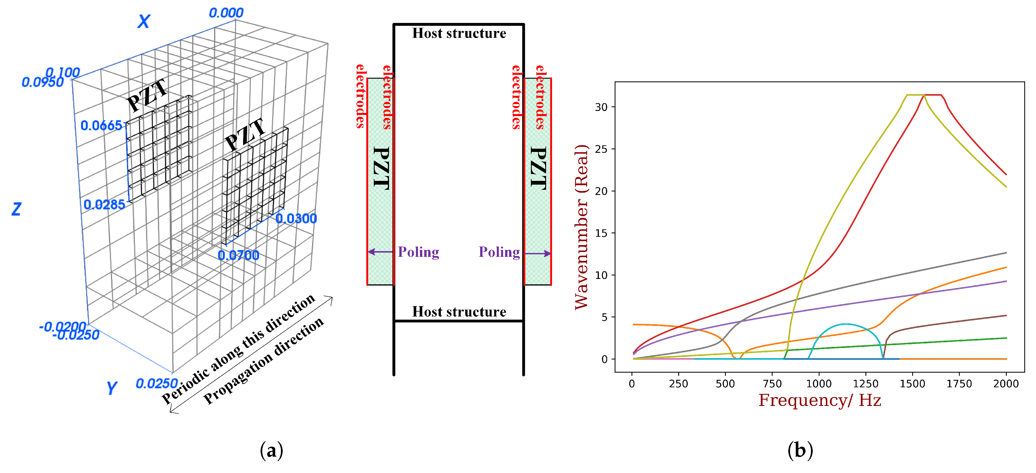
The considered thin-wall structure is shown in Figure 11a, with mesh quality verified by the forced response analysis [36]. Piezoelectric patches are periodically bonded and for each unit cell there are two PZT patches. The unit cell is then modeled by FEM, and for one single unit cell, the overall number of DOFs is 1896, with 336 on the left and right side, 1558 on the internal mechanical part and 2 on the electric part. The geometric parameters are also labelled on the figure by international units. The host and piezoelectric materials are the same as used in the previous section.
The dispersion curves in OC status are calculated from 0 to 2000 Hz by the full unit cell model, and the positive-going propagating waves are recognized and shown in Figure 11b. To obtain by definition, another calculation with SC status should be conducted, and the waves should be matched between OC and SC results. This is very difficult to programme as a general numerical tool. Here we select 3 waves for comparison, including both low-order (wave 0) and high-order waves (waves 4 and 5), and their results are computed by manually matching the waves. The results are computed by the reduced shapes associated with the reduced model as recommended in the previous section by the in-house Python code. The comparison of the results are shown in Figure 12 where a very good agreement is observed. The results acknowledge the statement that is a good approximation of and therefore consistent with MEMCF. The selected wave shapes are illustrated in Figure 13. The results verifies the use of WEMCF () for complex waveguides where complex wave shapes exist.
6. Application: Designing the Resistive PZT Waveguide
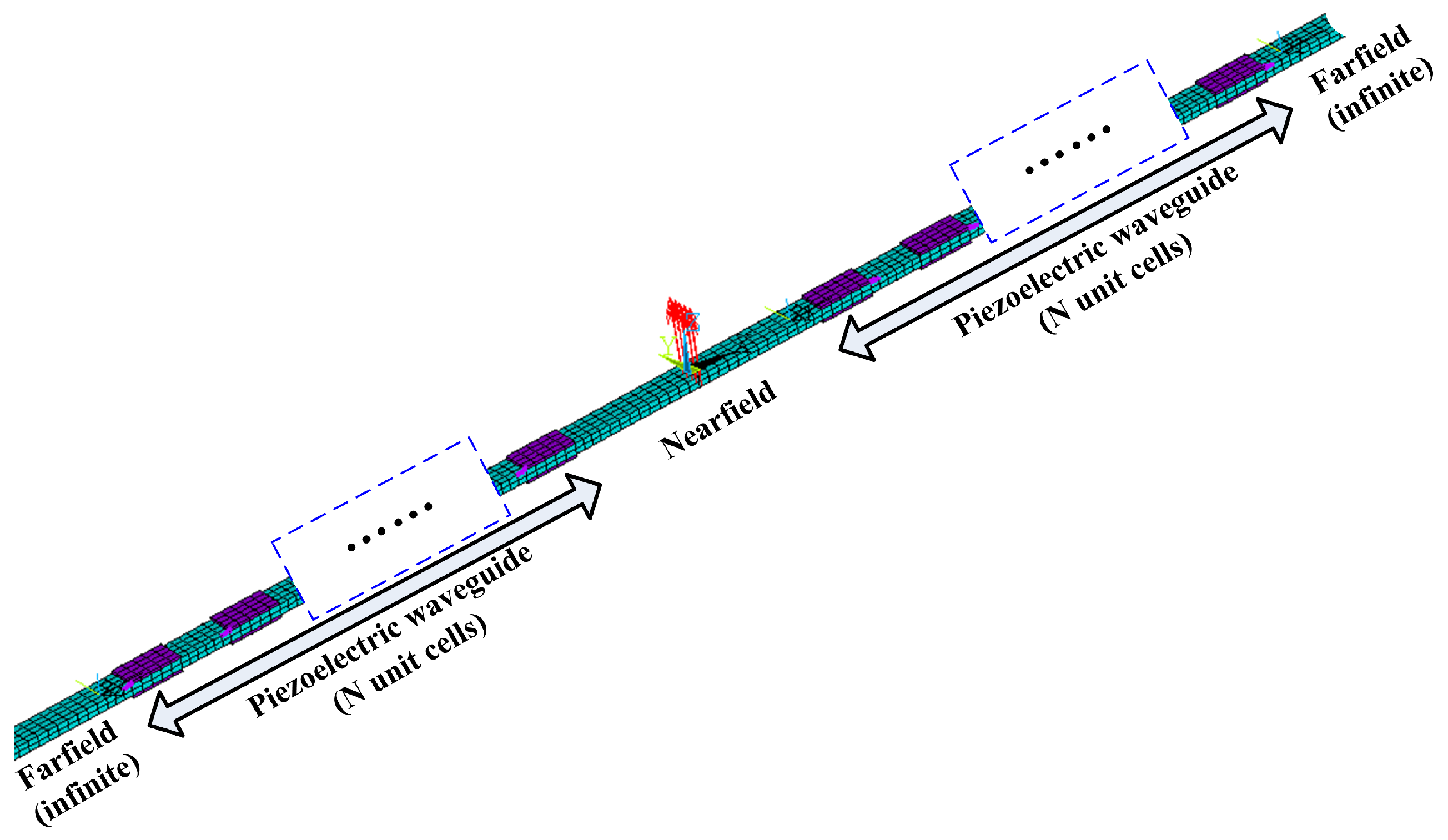
To illustrate the usage of the WEMCF, let us consider a built-up structure constructed by bonding groups of co-located piezoelectric patches onto a uniform host structure. N groups of piezoelectric patches are periodically distributed at the right side of the excitation while N other groups are located on the other side. The structure is infinite both to the left and right side. The FEM/WFEM hybrid method [31] can be used to analyse the energy flow and forced response. To do that, this structure is divided into five parts: one nearfield part, two piezoelectric waveguides and two uniform far-field waveguides, as shown in Figure 14.
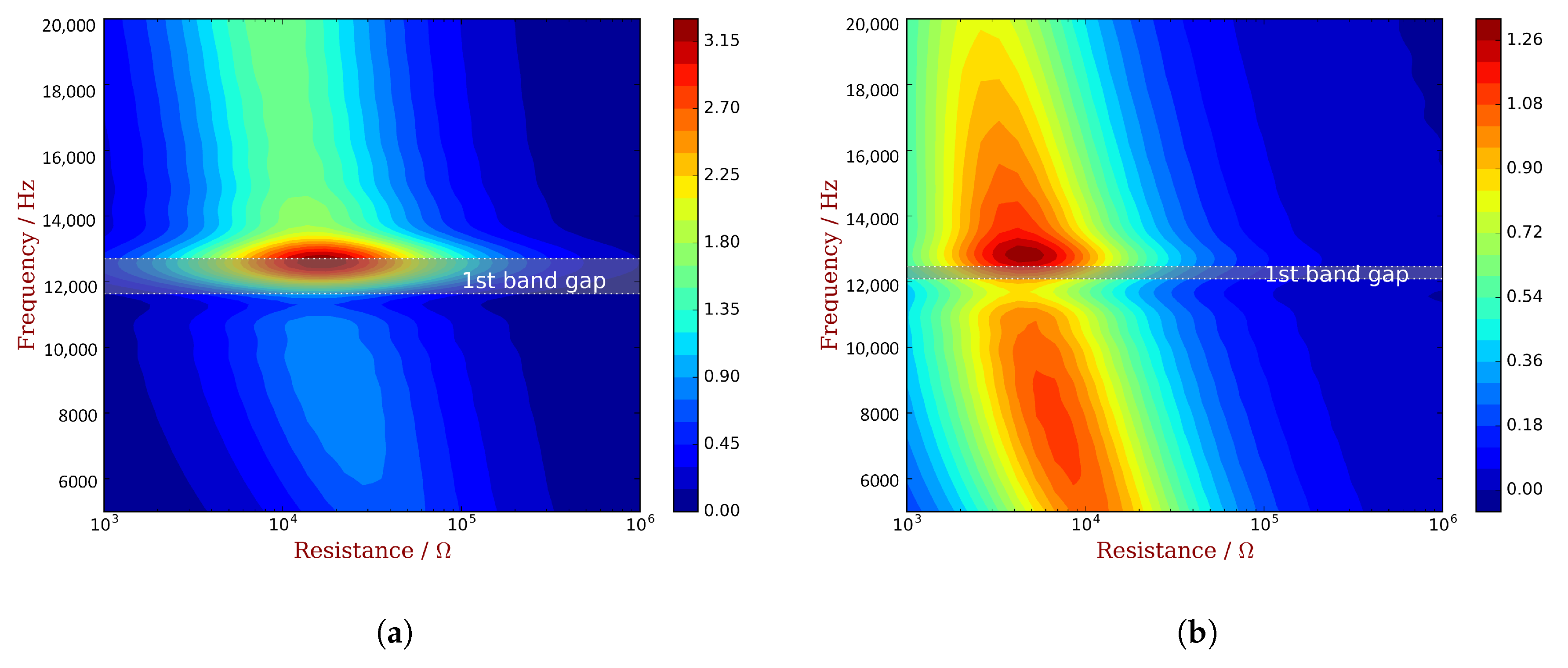
Here we fix . the external forces are applied in DOF of all the nodes that are located in the origin cross-section of the nearfield () with an amplitude of . The energy flow can be attenuated by shunting resistors to the PZT patches and this effects can be quantified by the power Transmission Loss (TL):
We conduct the parametric studies of TL with respect to the frequency and resistance. PZT waveguides with unit cell A and C are considered respectively, and the results are shown in Figure 15. It can be seen that the best TL and the associated resistance vary with frequency. Results also indicate some correlation between the best TL and the WEMCF: unit cell A has a better WEMCF in the second propagating zone; and the best TL is larger in the second propagating zone than in the first one, shown in Figure 15a; unit cell C has better WEMCF in the first propagating zone than the second, and a lower best TL can be observed in higher frequencies.
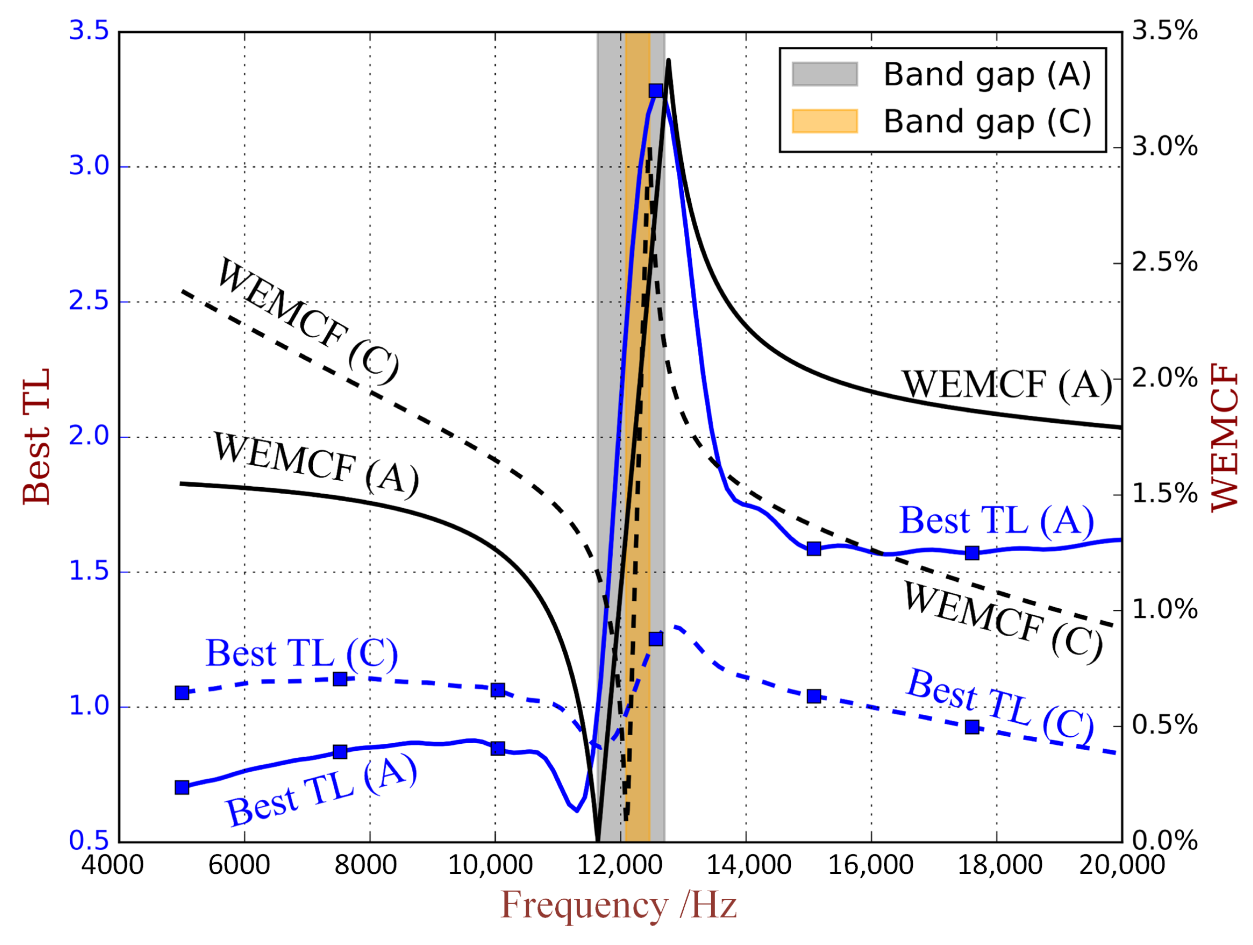
To illustrate this correlation more clearly, we plot the best TL with respect to the frequency when using unit cells A and C in Figure 16, in association with the WEMCF of wave 0 of unit cell A and C. In the first propagating zone, we can see that unit cell A has stronger WEMCF than C, and the best TL when using A is better than C. In the second propagating zone, we can see that unit cell A has weaker WEMCF than C, and the best TL when using A is weaker than C.
This correlation between WEMCF and best TL allows to compare configurations of unit cell without performing the forced response and energy analysis of the built-up structure. It means the design for the geometric and electric parameters can be done separately: first we determine the geometric parameters so as to achieve the best WEMCF, only by free-wave analysis; then we only consider the unit cell with optimized geometrics to determine the electric parameters so as to achieve the best power attenuation.
7. Conclusions
In this paper, we study the factor that allows to quantify the coupling strength between the mechanical and electric fields during the passage of a wave in piezoelectric composites, termed the wave electromechanical coupling factor (WEMCF). We show that to maintain the consistency with the classical modal electromechanical coupling factor (MEMCF), the WEMCF should also be defined by the frequency difference of the OC and SC statues. However, this definition has difficulties in calculation for general piezoelectric waveguide for the need of computing dispersion curves twice and matching waves between SC and OC statuses.
To address this challenge, an effective energy formula for WEMCF is proposed, defining the WEMCF as the percentage of electric energy stored in the free intrinsic capacitance over the mechanical energy during the passage of the wave. This energy formula is a good approximation to the frequency formula, and we only need to analyze the dispersion curves once and do not need to match waves from different electrode statuses.
The proposed energy formula can be calculated as a post-processing of the wave and finite element method. We recommend the use of reduced wave shapes for a fast calculation of WEMCF. It reduces the CPU time for computing WEMCF of the example structure to less than 1%, and it works for complex structures. Please note that the method can be used in any frequency ranges, provided that an appropriate FE model for the unit cell is established.
An application is given, concerning the energy flow attenuation in a built-up structure by resistive PZT shunts. We show that the WEMCF is strongly correlated with the best energy transmission loss. This provides more insights to understand the waveguide performance and it also allows the design of the geometric and electric parameters to be done separately.
Supplementary Materials
The following are available online at https://www.mdpi.com/1996-1944/11/8/1406/s1: File ‘APDL_UC_A.txt’—Code in ANSYS parametric design language (APDL) for unit cell A used in the paper. File APDL_UC_B.txt—Code in APDL for unit cell B. File ‘APDL_UC_C.txt’—Code in APDL for unit cell C. File ‘APDL_UC_Thin_wall.txt’—Code in APDL for the piezoelectric thin-wall structure.
Author Contributions
Conceptualization, Y.F. and M.C.; Methodology, Y.F. and M.C.; Software, Y.F. and O.B.; Validation, Y.F. and O.B.; Writing—Original Draft Preparation, Y.F.; Writing—Review & Editing, M.I. and L.L.; Supervision, M.I. and M.C.; Project Administration, L.L.; Funding Acquisition, L.L. and Y.F.
Funding
This research was funded by National Natural Science Foundation of China under Grant numbers 51675022 and 11702011, and China Post-doctoral Science Foundation under grant numbers 2017M610741 and 2018T110032.
Conflicts of Interest
The authors declare no conflict of interest. The founding sponsors had no role in the design of the study; in the collection, analyses, or interpretation of data; in the writing of the manuscript, and in the decision to publish the results.
Abbreviations
The following abbreviations are used in this manuscript:
| EMCF | electromechanical coupling factor |
| WEMCF | wave electromechanical coupling factor |
| MEMCF | modal electromechanical coupling factor |
| WFEM | wave and finite element method |
| FRF | frequency response function |
| TL | transmission loss |
| OC | open circuit |
| SC | short circuit |
| DOF | Degree-of-freedom |
Appendix A. Material Properties of the Piezoelectric Material (PZT4)
Mass density:
Material stiffness matrix evaluated at constant electric field:
Permittivity matrix evaluated at constant strain:
where .
Piezoelectric stress coupling matrix:
References
- Priya, S.; Inman, D.J. (Eds.) Energy Harvesting Technologies; Springer: Boston, MA, USA, 2009; pp. 325–336. [Google Scholar]
- Qin, Q.H. Advanced Mechanics of Piezoelectricity; Higher Education Press: Beijing, China, 2012. [Google Scholar]
- Berlincourt, D.A.; Curran, D.R.; Jaffe, H. Piezoelectric and Piezomagnetic Materials and Their Function in Transducers. In Physical Acoustics; Elsevier: New York, NY, USA, 1964; pp. 169–270. [Google Scholar]
- IEEE. IEEE Standard on Piezoelectricity; IEEE: Piscataway, NJ, USA, 1988. [Google Scholar]
- Wasa, K.; Ito, S.; Nakamura, K.; Matsunaga, T.; Kanno, I.; Suzuki, T.; Okino, H.; Yamamoto, T.; Seo, S.H.; Noh, D.Y. Electromechanical coupling factors of single-domain 0.67Pb(Mg1/3Nb2/3)O3-0.33PbTiO3 single-crystal thin films. Appl. Phys. Lett. 2006, 88, 122903. [Google Scholar] [CrossRef] [Green Version]
- Pijolat, M.; Loubriat, S.; Queste, S.; Mercier, D.; Reinhardt, A.; Defaÿ, E.; Deguet, C.; Clavelier, L.; Moriceau, H.; Aïd, M.; et al. Large electromechanical coupling factor film bulk acoustic resonator with X-cut LiNbO3 layer transfer. Appl. Phys. Lett. 2009, 95, 182106. [Google Scholar] [CrossRef]
- Mason, W.P.; Baerwald, H. Piezoelectric Crystals and Their Applications to Ultrasonics. Phys. Today 1951, 4, 23. [Google Scholar] [CrossRef]
- Preumont, A. Dynamics of Electromechanical and Piezoelectric Systems; Springer: Dordrecht, The Netherlands, 2006; p. 224. [Google Scholar]
- Thomas, O.; Ducarne, J.; Deü, J.F. Performance of piezoelectric shunts for vibration reduction. Smart Mater. Struct. 2012, 21, 015008. [Google Scholar] [CrossRef] [Green Version]
- Vasques, C.M.A. Improved passive shunt vibration control of smart piezo-elastic beams using modal piezoelectric transducers with shaped electrodes. Smart Mater. Struct. 2012, 21, 125003. [Google Scholar] [CrossRef]
- Ducarne, J.; Thomas, O.; Deü, J.F. Placement and dimension optimization of shunted piezoelectric patches for vibration reduction. J. Sound Vib. 2012, 331, 3286–3303. [Google Scholar] [CrossRef]
- Li, L.; Yin, S.; Liu, X.; Li, J. Enhanced electromechanical coupling of piezoelectric system for multimodal vibration. Mechatronics 2015, 31, 205–214. [Google Scholar] [CrossRef]
- Mead, D. Waves and Modes in Finite Beams: Application of the Phase-Closure Principle. J. Sound Vib. 1994, 171, 695–702. [Google Scholar] [CrossRef]
- Langley, R. Some perspectives on wave-mode duality in SEA. In Proceedings of the IUTAM International Symposium on Statistical Energy Analysis, Southampton, UK, 8–11 July 1997; pp. 1–12. [Google Scholar]
- Wang, X.; So, R.; Chan, K. Resonant beam vibration: A wave evolution analysis. J. Sound Vib. 2006, 291, 681–705. [Google Scholar] [CrossRef]
- Collet, M.; Cunefare, K.; Ichchou, M. Wave Motion Optimization in Periodically Distributed Shunted Piezocomposite Beam Structures. J. Intell. Mater. Syst. Struct. 2008, 20, 787–808. [Google Scholar] [CrossRef]
- Tateo, F.; Collet, M.; Ouisse, M.; Ichchou, M.; Cunefare, K.; Abbe, P. Experimental characterization of a bi-dimensional array of negative capacitance piezo-patches for vibroacoustic control. J. Intell. Mater. Syst. Struct. 2015, 26, 952–964. [Google Scholar] [CrossRef]
- Chen, S.; Wang, G.; Wen, J.; Wen, X. Wave propagation and attenuation in plates with periodic arrays of shunted piezo-patches. J. Sound Vib. 2013, 332, 1520–1532. [Google Scholar] [CrossRef]
- Dai, L.; Jiang, S.; Lian, Z.; Hu, H.; Chen, X. Locally resonant band gaps achieved by equal frequency shunting circuits of piezoelectric rings in a periodic circular plate. J. Sound Vib. 2015, 337, 150–160. [Google Scholar] [CrossRef]
- Bareille, O.; Kharrat, M.; Zhou, W.; Ichchou, M. Distributed piezoelectric guided-T-wave generator, design and analysis. Mechatronics 2012, 22, 544–551. [Google Scholar] [CrossRef]
- Thien, A.B.; Chiamori, H.C.; Ching, J.T.; Wait, J.R.; Park, G. The use of macro-fibre composites for pipeline structural health assessment. Struct. Control Health Monit. 2008, 15, 43–63. [Google Scholar] [CrossRef]
- Su, Z.; Ye, L. Selective generation of Lamb wave modes and their propagation characteristics in defective composite laminates. Proc. Inst. Mech. Eng. Part L 2004, 218, 95–110. [Google Scholar] [CrossRef]
- Mueller, I.; Fritzen, C.P. Inspection of Piezoceramic Transducers Used for Structural Health Monitoring. Materials 2017, 10, 71. [Google Scholar] [CrossRef] [PubMed]
- Ono, K. On the Piezoelectric Detection of Guided Ultrasonic Waves. Materials 2017, 10, 1325. [Google Scholar] [CrossRef] [PubMed]
- Chen, S.; Zhang, Y.; Lin, S.; Fu, Z. Study on the electromechanical coupling coefficient of Rayleigh-type surface acoustic waves in semi-infinite piezoelectrics/non-piezoelectrics superlattices. Ultrasonics 2014, 54, 604–608. [Google Scholar] [CrossRef] [PubMed]
- Fan, L.; Zhang, S.Y.; Zheng, K.; Lin, W.; Gao, H.D. Calculation of electromechanical coupling coefficient of Lamb waves in multilayered plates. Ultrasonics 2006, 44 (Suppl. 1), e849–e852. [Google Scholar] [CrossRef] [PubMed]
- Fan, Y.; Collet, M.; Ichchou, M.; Li, L.; Bareille, O.; Dimitrijevic, Z. A wave-based design of semi-active piezoelectric composites for broadband vibration control. Smart Mater. Struct. 2016, 25, 055032. [Google Scholar] [CrossRef]
- Chang, S.; Rogacheva, N.; Chou, C. Analysis of methods for determining electromechanical coupling coefficients of piezoelectric elements. IEEE Trans. Ultrason. Ferroelectr. Freq. Control 1995, 42, 630–640. [Google Scholar] [CrossRef]
- Mead, D. Wave propagation and natural modes in periodic systems: II. Multi-coupled systems, with and without damping. J. Sound Vib. 1975, 40, 19–39. [Google Scholar] [CrossRef]
- Fan, Y.; Zhou, C.; Laine, J.; Ichchou, M.; Li, L. Model reduction schemes for the wave and finite element method using the free modes of a unit cell. Comput. Struct. 2018, 197, 42–57. [Google Scholar] [CrossRef]
- Fan, Y.; Collet, M.; Ichchou, M.; Li, L.; Bareille, O.; Dimitrijevic, Z. Energy flow prediction in built-up structures through a hybrid finite element/wave and finite element approach. Mech. Syst. Signal Proc. 2016, 66-67, 137–158. [Google Scholar] [CrossRef]
- Mead, D. The forced vibration of one-dimensional multi-coupled periodic structures: An application to finite element analysis. J. Sound Vib. 2009, 319, 282–304. [Google Scholar] [CrossRef]
- Zhou, C.W.; Lainé, J.P.; Ichchou, M.; Zine, A.M. Wave finite element method based on reduced model for periodic structures. Int. J. Appl. Mech. 2015, 07, 1550018. [Google Scholar] [CrossRef]
- Mencik, J.M. New advances in the forced response computation of periodic structures using the wave finite element (WFE) method. Comput. Mech. 2014, 54, 789–801. [Google Scholar] [CrossRef] [Green Version]
- Waki, Y.; Mace, B.; Brennan, M. Numerical issues concerning the wave and finite element method for free and forced vibrations of waveguides. J. Sound Vib. 2009, 327, 92–108. [Google Scholar] [CrossRef]
- Fan, Y.; Collet, M.; Ichchou, M.; Li, L.; Bareille, O.; Dimitrijevic, Z. Enhanced wave and finite element method for wave propagation and forced response prediction in periodic piezoelectric structures. Chin. J. Aeronaut. 2017, 30, 75–87. [Google Scholar] [CrossRef]
- Benjeddou, A. Advances in piezoelectric finite element modeling of adaptive structural elements: A survey. Comput. Struct. 2000, 76, 347–363. [Google Scholar] [CrossRef]
- Zhou, C. Wave and Modal Coupled Approach for Multi-Scale Analysis of Periodic Structures. Ph.D. Thesis, Ecole Centrale de Lyon, Ecully, France, 2014. [Google Scholar]
- Mead, D. A general theory of harmonic wave propagation in linear periodic systems with multiple coupling. J. Sound Vib. 1973, 27, 235–260. [Google Scholar] [CrossRef]
Figure 1.
Illustration of dispersion curves for OC and SC status of a piezoelectric waveguide.

Figure 2.
Illustration of the unit cells in a piezoelectric waveguide.
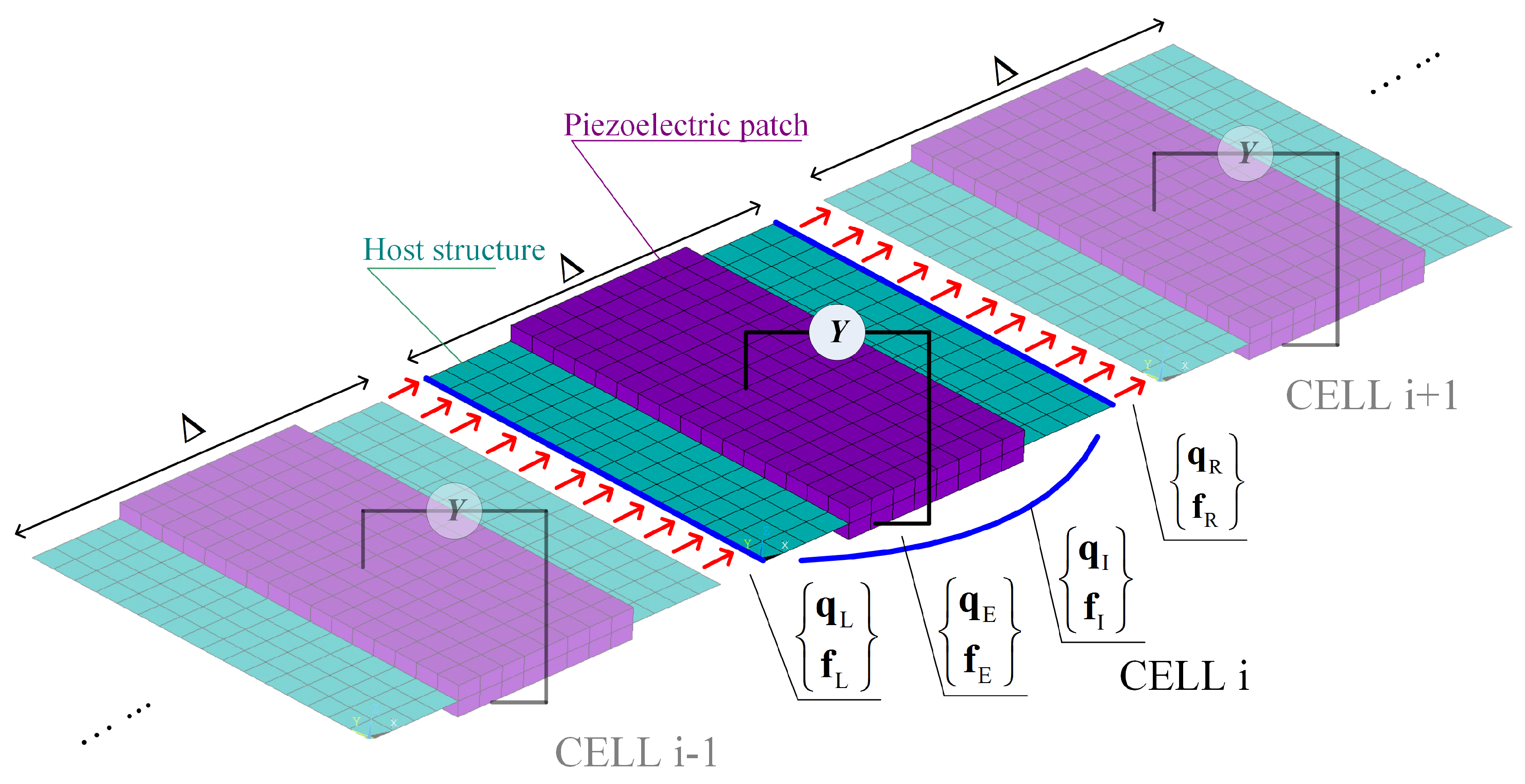
Figure 3.
Illustration of different paths for the calculation of WEMCF in the framework of WFEM.
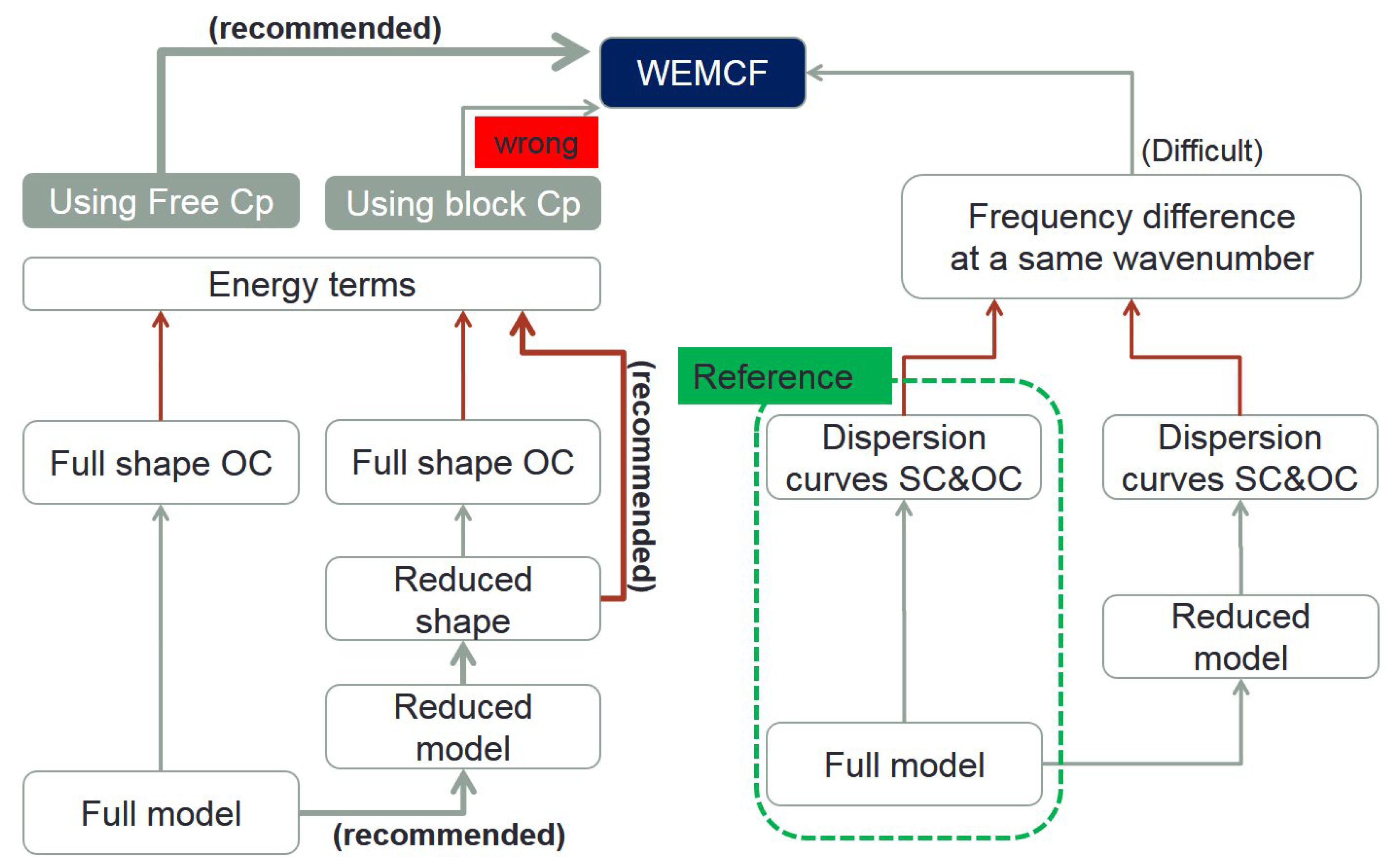
Figure 4.
Unit cells of the piezoelectric waveguides: (a) unit cell A; (b) unit cell B which is a non-symmetric way of choosing the unit cell for the infinite periodic structure with unit cell A; (c) unit cell C which has longer PZT patches. The Piezoelectric materials are polarized along the z axis, and the electrodes fully cover the surfaces parallel to the x-y plane (orthogonal to the polarized direction). The program code used to generate the Finite Element models in ANSYS can be found in the Supplementary Files.

Figure 5.
Comparison of WEMCF calculated by using: full WFEM with (labelled by ‘Reference’), full WFEM with (labelled by ‘using ’), full WFEM with (labelled by ‘using ’) and reduced waveshape with (labelled by ‘using (reduced)’).
Figure 5.
Comparison of WEMCF calculated by using: full WFEM with (labelled by ‘Reference’), full WFEM with (labelled by ‘using ’), full WFEM with (labelled by ‘using ’) and reduced waveshape with (labelled by ‘using (reduced)’).

Figure 6.
Dispersion curves and WEMCF for the piezoelectric waveguide with unit cell A: only wave 0 (z transverse) and 3 (longitudinal) have significant values.
Figure 6.
Dispersion curves and WEMCF for the piezoelectric waveguide with unit cell A: only wave 0 (z transverse) and 3 (longitudinal) have significant values.

Figure 7.
Waveshape of wave 0 of unit cell A at the border frequencies of the band gaps: (a) , low WEMCF; (b) , high WEMCF; (c) , low WEMCF; (d) , high WEMCF.
Figure 7.
Waveshape of wave 0 of unit cell A at the border frequencies of the band gaps: (a) , low WEMCF; (b) , high WEMCF; (c) , low WEMCF; (d) , high WEMCF.
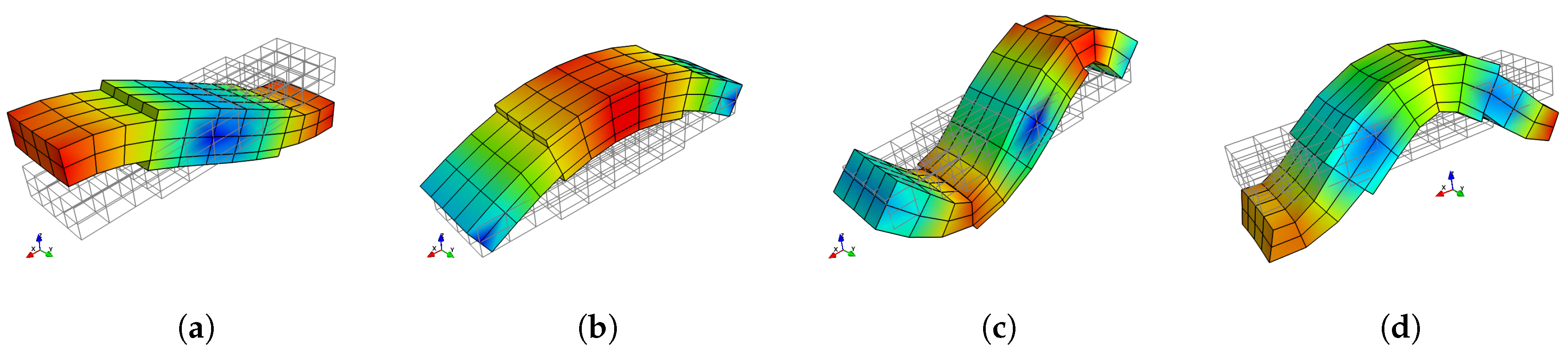
Figure 8.
CPU time for the full dispersion characteristics with WFEM of unit cell A by the energy formula where the energies are calculated by: (1) using full shapes obtained from full WFEM; (2) using full shapes obtained from reduced WFEM; (3) using reduced shapes. The label ’Wave selection and matching’ refers to the standard post-processing of the WFEM results in order to identify the same type of wave among different frequencies [36], not the matching between the results between the OC and SC status as required for computing the frequency formula of WEMCF.

Figure 9.
Dispersion curves and WEMCF for the piezoelectric waveguide with unit cell C.

Figure 10.
Waveshape of wave 0 of unit cell C: (a) at the first propagating zone; (b) at the second propagating zone.
Figure 10.
Waveshape of wave 0 of unit cell C: (a) at the first propagating zone; (b) at the second propagating zone.
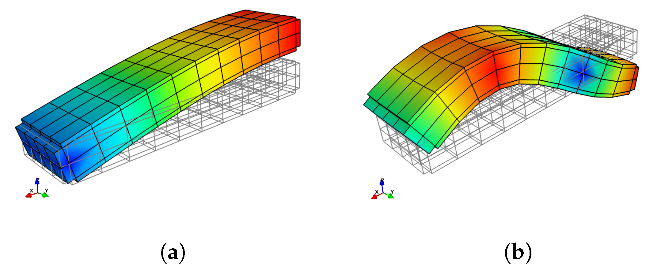
Figure 11.
The unit cell of the thin-wall piezoelectric structure (a) and its dispersion curves (b). The program code used to generate the Finite Element model in ANSYS can be found in the Supplementary Files.
Figure 11.
The unit cell of the thin-wall piezoelectric structure (a) and its dispersion curves (b). The program code used to generate the Finite Element model in ANSYS can be found in the Supplementary Files.

Figure 12.
The comparison of WEMCF calculated by the frequency formula and the energy formula . Waves 0, 4 and 5 are selected from the full dispersion curves in Figure 11b. The is calculated by the reduced wave shapes as recommended in the last section.
Figure 12.
The comparison of WEMCF calculated by the frequency formula and the energy formula . Waves 0, 4 and 5 are selected from the full dispersion curves in Figure 11b. The is calculated by the reduced wave shapes as recommended in the last section.
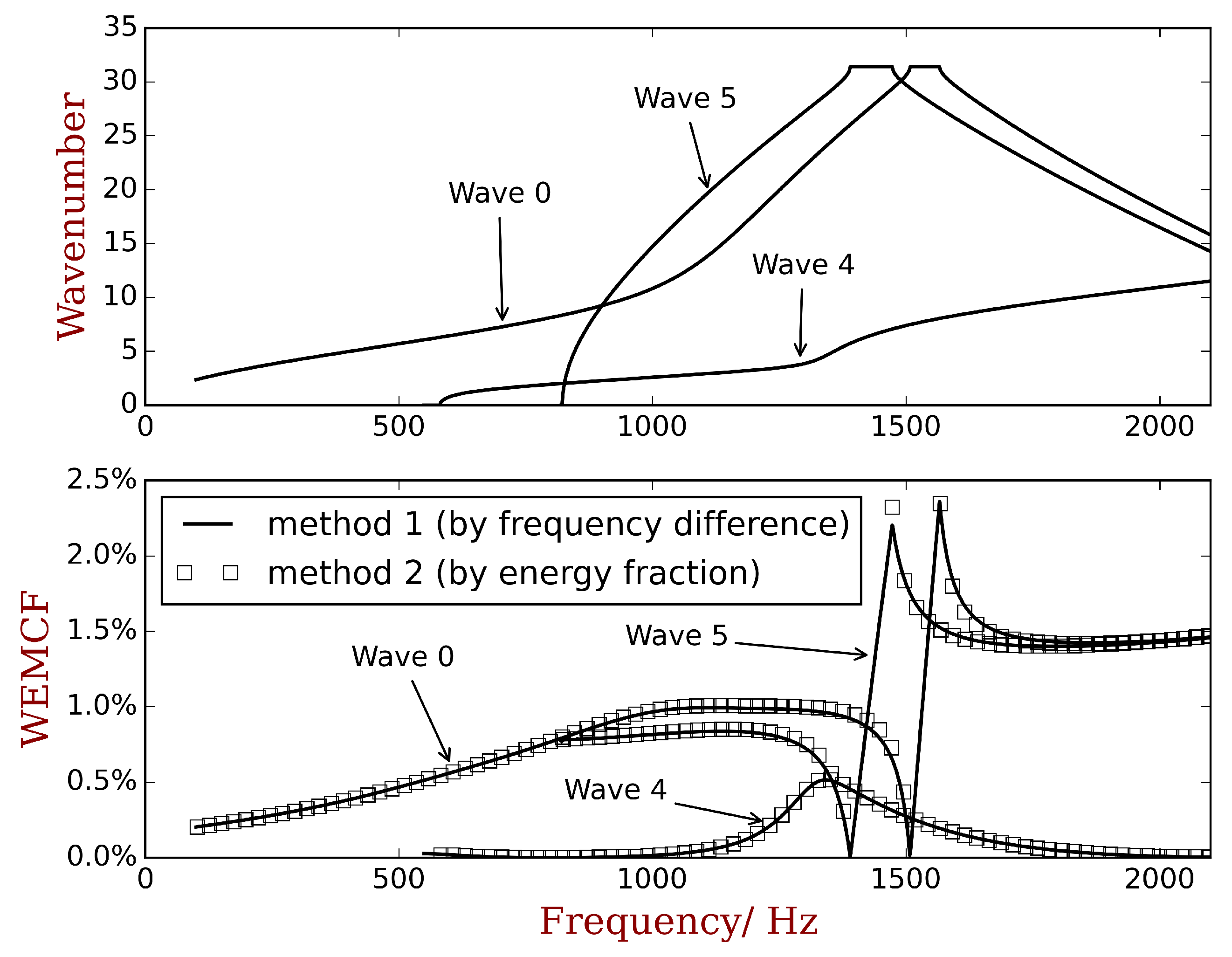
Figure 13.
Wave shapes of the at 1000 : (a) wave 0; (b) wave 4; (c) wave 5.
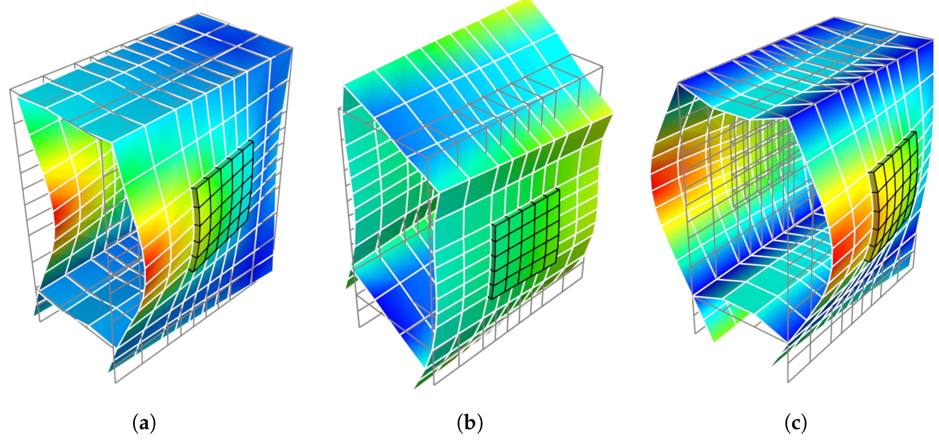
Figure 14.
The considered built-up structure and the dividing of substructures.

Figure 15.
Parametric study of power transmission loss with respect to frequency and resistance, when the piezoelectric waveguides use: (a) unit cell A; (b) unit cell C.
Figure 15.
Parametric study of power transmission loss with respect to frequency and resistance, when the piezoelectric waveguides use: (a) unit cell A; (b) unit cell C.

Figure 16.
The best TL and WEMCF with respect to the frequency for PZT waveguide with unit cell A and unit cell C.
Figure 16.
The best TL and WEMCF with respect to the frequency for PZT waveguide with unit cell A and unit cell C.
© 2018 by the authors. Licensee MDPI, Basel, Switzerland. This article is an open access article distributed under the terms and conditions of the Creative Commons Attribution (CC BY) license (http://creativecommons.org/licenses/by/4.0/).
Share and Cite
MDPI and ACS Style
Fan, Y.; Collet, M.; Ichchou, M.; Bareille, O.; Li, L. Wave Electromechanical Coupling Factor for the Guided Waves in Piezoelectric Composites. Materials 2018, 11, 1406. https://doi.org/10.3390/ma11081406
AMA Style
Fan Y, Collet M, Ichchou M, Bareille O, Li L. Wave Electromechanical Coupling Factor for the Guided Waves in Piezoelectric Composites. Materials. 2018; 11(8):1406. https://doi.org/10.3390/ma11081406
Chicago/Turabian StyleFan, Yu, Manuel Collet, Mohamed Ichchou, Olivier Bareille, and Lin Li. 2018. "Wave Electromechanical Coupling Factor for the Guided Waves in Piezoelectric Composites" Materials 11, no. 8: 1406. https://doi.org/10.3390/ma11081406
Note that from the first issue of 2016, this journal uses article numbers instead of page numbers. See further details here.