Some Considerations about the Use of Contact and Confocal Microscopy Methods in Surface Texture Measurement

 , , and
Abstract
:1. Introduction
2. Evaluation Procedure of Roughness Parameters
2.1. Parameters Calculation
- 1.
- Obtaining the extracted profile measured by different instruments. The file contains the sampled coordinates and the digitized coordinates .
- 2.
- Form removal. Due to the impossibility of placing the measured profile fully parallel to the measurement base, or the presence of geometric errors on the surface of the measurand, it is necessary to eliminate this form by fitting the data to a nominal shape (line, polynomial, and circle). Correction can be done in two ways: applying a tilt correction or by subtraction of the mean. This one will be used when the angle rotated by the surface is very small. The coordinates are obtained. When the fitting to a regression line is employed, its mathematical representation is:The coefficients and can be calculated using the least squares method. The line that best fits the set of coordinates is:where is the residual. It is possible to solve a linear system, obtaining the coefficients and , using:Using the same procedure, it is possible to eliminate the form of surfaces that can be adjusted to quadratic polynomials.
- 3.
- Filter. The profile is filtered using a low pass filter with a cut-off. The primary profile is obtained with coordinates .
- 4.
- Filter. The profile is now filtered using a high pass filter with a cut-off according to the standard ISO 16610-21 [18]. This way, the waviness profile is eliminated, obtaining the roughness profile with coordinates .
- 5.
- Obtaining the roughness parameters, according to the standards ISO 4287 [19] and ISO 4288 [20]. In order to solve the calculation of the equations described in the aforementioned standards (roughness parameters Ra, Rq, Rsk, and Rku), a method of integral analytical calculation, the trapezoidal method, has been used instead of the formula of discrete calculation (Equations (8)–(11)) to improve the accuracy of the results.Parameters Rt, Rz, Rp, and Rv measure the amplitude of the profile (peak and valley distances), Ra is used to calculate the average roughness, Rq measures the variance of the amplitude distribution function (ADF) of the profile, Rsk analyze the asymmetry of the ADF, and Rku evaluates the spikiness of the profile.Depending on the type of instrument evaluated, different coordinates will be generated, so it will not be necessary to execute all steps.
2.2. Model for Calculating Uncertainties
- 1.
- Definition of the output quantities. Parameters Rt, Rz, Rp, Rv, Ra, Rq, Rsk, Rku, and RSm.
- 2.
- Definition of input quantities. The sampled coordinates and the digitized coordinates, and scale division error of the instrument on the z-axis. In this work, only the sources that directly affect the coordinates of the captured profile, and therefore the variability of the measurements, have been taken into account.All of these magnitudes analyze the variations generated by the instrument in the measurements: noise in the readings, imperfections in the reference of the instrument, sampling and digitizing process, and rounding-off of the coordinates and software calculations, as well as the horizontal and vertical resolution of the instrument and the idealization of the Gaussian filter [26,27].
- 3.
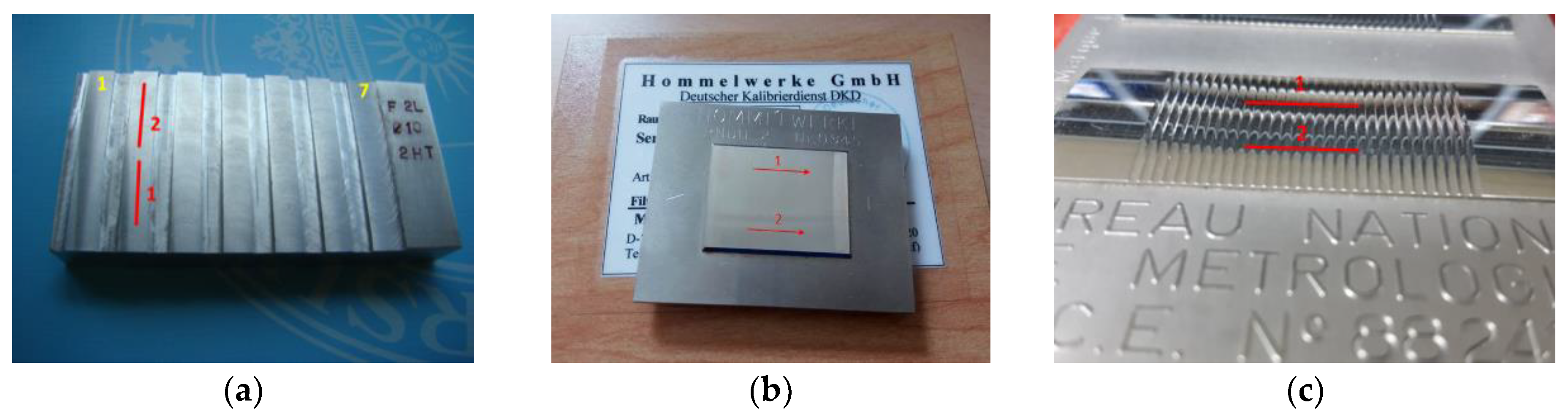
- Assignment of the probability density functions (PDF) to the input variables. For the input variables defined above, it is established that variability due to the process of obtaining the sampled coordinates responds to a normal distribution with a mean of the raw coordinate value and a standard deviation equal to 2% of the sampling step [28,29].In order to analyze the variability of the z-coordinates, it was necessary to perform a repeatability study of the measurements [30]. That is to say, measuring the same profile a large number of times, by the same operator, with the same measurement procedure, same measuring system, and same operation conditions [31].After doing different experiments, it has been observed that it is practically impossible to obtain the same position of the z-coordinate to be analyzed. Therefore, an analysis of the repeatability of the parameters Pp and Pv is planned, where the parameters Pp and Pv are the maximum profile peak height of the primary profile and maximum profile valley depth of the primary profile, respectively. For this type C1 spacing standard, grooves having a sine wave profile will be measured and the standard deviations of the previous parameters will be determined. This study assumes that this variability corresponds to a t-distribution (employed when a series of indications are evaluated). The standard uncertainty associated with this variability can be estimated as:where is the maximum standard deviation of the parameters Pp and Pv, obtained in the experiment, is the degrees of freedom of the obtained parameters, and represents the numbers of measurements made in the roughness measurement (typically one).Therefore, the digitized coordinates respond to a t-distribution of the mean value of the raw coordinate z and a standard uncertainty equal to the value calculated by the previous equation. The experimental values obtained are shown in Section 4.The scale division errors of the instrument on the z-axis, responds to a rectangular distribution of limits , where is the scale division on the z-axis.
- 4.
- Propagation. According to the recommendation of Supplement 1 to the GUM, in its Section 7.2.3, it is possible to use a small number of iterations () for complex models. Taking into account this recommendation, the standard deviation and the mean of the values obtained after performing the iterations of the model, could be taken as and respectively, and can be assigned to a Gaussian PDF . In the simulations, 10,000 replications have been performed, requiring between 2 and 70 min of calculation on a computer with an i7-6700HQ-Intel(R) Core(TM) and 16 GB memory.
- 5.
- Results. The standard deviation of the resulting values obtained in the simulations, as well as their mean, is calculated. To determine the amplitude of the coverage interval, the minimum interval method is used [32,33]. Using the suggestions of Supplement 2 of the GUM, it is possible to determine the covariance matrix of the calculated parameters (all parameters will be correlated to a certain degree, due to the presence of common input variables in all of them). From the covariance matrix it is possible to calculate the matrix of correlation coefficients .
2.3. Algorithm Validation
3. Methodology of Experimental Study on Roughness
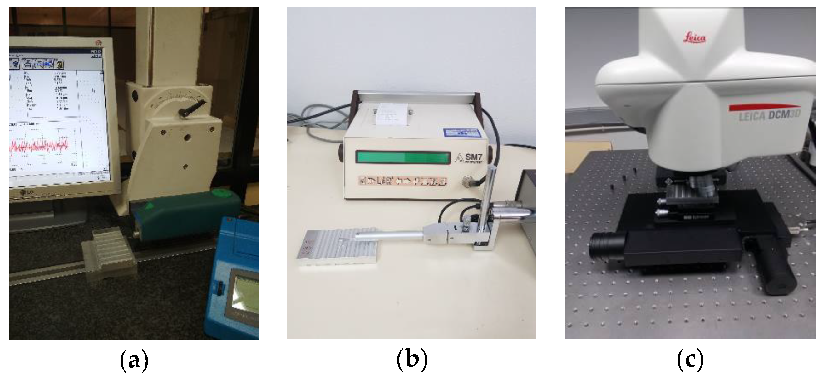
- Stylus profilometer 1 (SP-1): portable stylus profilometer with a mechanical probe, brand HOMMELWERKE, model TESTER T1000 WAVE with probe TKL 300L, stylus tip of 5 µm/90°. Measuring range: ±80 µm/±320 µm. Vertical resolution (Z): 0.01 µm/0.04 µm. Transverse length: 0.05–20 mm. X sampling: 0.583 µm (Figure 3a).
- Stylus profilometer 2 (SP-2): portable stylus profilometer with a mechanical probe, brand SM, model PROFILTEST SM7 with stylus tip of 5 µm. Measuring range: 320 µm. Vertical resolution (Z): 0.01 µm. X sampling: 2.5 µm (Figure 3b).
- Confocal microscope (CM-3) confocal microscope, brand Leica (Wetzlar, Germany), model DCM-3D. It uses episcopic illumination, with light source LED type of wavelength 460 nm. Image Acquisition Sensor: monochrome CCD for confocal applications. The equipment has five lenses, with amplification between 5× and 150×. A 50× lens was used in the measurements to provide agreement between amplification and data acquisition speed. This lens has the following characteristics: Measuring field: 254.64 × 190.90 µm. Pixel size: 0.332 µm and equal to the lateral resolution (XY). Vertical resolution (Z): <3 nm. Total measuring field of instrument: 114 × 75 × 40 mm (Figure 3c).
4. Analysis of Experimental Results
4.1. Tactile Method
- Measuring ranges: In height (z-axis), the smallest measuring field allowed by each instrument has been selected. In length (x-axis), a profile of length of 5.6 mm (7× ) has been evaluated.
- Operating time: The effective measurement time, which included the movement of the probe on the surface, the calculation of parameters by the equipment, and the saving of the data files, has been less than 2 min. The preparation time of the sample, which includes the positioning and inclination adjustment by rotation of the SP-1 probing system (Figure 3a), lasted 10 min at most.
- Environmental considerations: Regarding the SP-1 and SP-2 environmental requirements, the measurements were carried out at a controlled temperature of 20 ± 1 °C
- Measurand preparation: It included the cleaning of the measurand by a mixture of alcohol and ether, as well as the correct placement of the measurand on the basis of measurement (indicated in the previous point). Prior to measurement, the part had been thermally stabilized for at least 3 h.
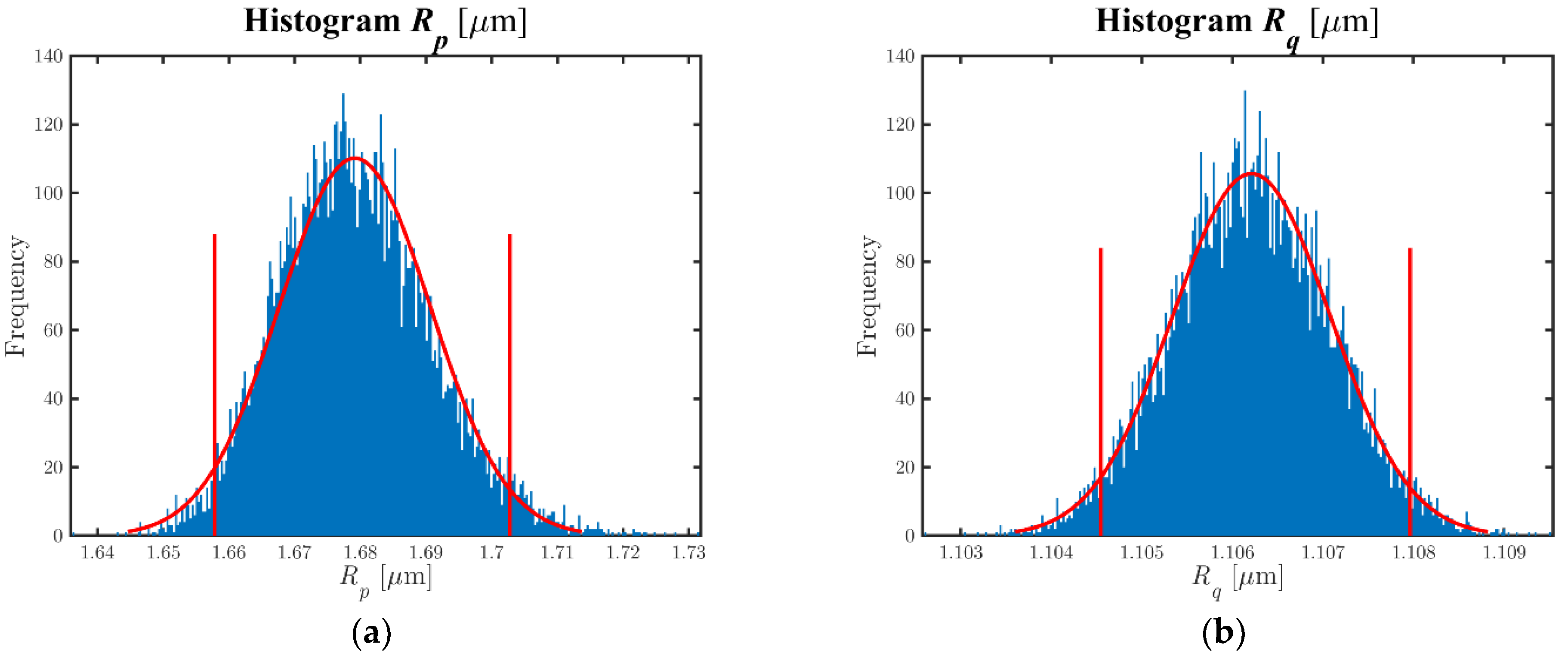
- Numeric values of the parameters: Table 4 shows, as an example, the results of measurand 8 when it was measured with the SP-1 equipment for a simulation performed for = 104. Figure 4a,b show, by way of example, the histograms of parameters Rp and Rq. It was verified that these parameters can be reasonably approximated to a normal distribution. Analogous behavior was obtained for the other parameters. Table 5 shows the correlation coefficients matrix of the roughness parameters, verifying the presence of correlation between them. Some of them show high correlation coefficient values (>0.5), due to the fact that all the parameters employ the same input quantities, that is to say, raw coordinates . Table 6 (columns 2 and 4) and Table 7 (columns 2 and 4) show some of the values obtained in the measurements of the different measurands after applying the algorithm used for the evaluation of roughness parameters. As it can be observed, there were discrepancies between the values of the equipment, higher for the amplitude parameters (peak and valley), presenting differences between 11% and 17% of the value analyzed and minimal when evaluating the amplitude parameter (average of ordinates), with differences in percentage between 0.2% and 4%. The difference in the spacing parameter was due to the different x sampling value of each piece of equipment. When comparing measurands, better amplitude parameter results (average of ordinates) were obtained when a standard was evaluated (measurand 8). When the piece was measured, differences up to 12% were obtained due to the impossibility of measuring the same profile with different equipment, and the presence of irregularities in the surface of the piece. The uncertainty of the parameters was similar when a standard or a piece was measured. The amplitude parameters (peak and valley) presented values of uncertainty of hundredths of a micrometer and were at least one or two orders of magnitude higher than the uncertainty of the amplitude parameters (average of ordinates). This was due to the process of obtaining these parameters.
- Data storage requirements: The data file, ASC/.txt extension, presented 9598/2241 rows of values, providing coordinates /step and / coordinates, with a file size of 260/25 kB (SP-1/SP-2).
- Cost of instrumentation/maintenance: The acquisition cost of the equipment was 12,000/6000 €. The maintenance was practically non-existent (lubrication of the vertical slide guides of the probing head for the SP-1 equipment).
4.2. Confocal Microscope
- Measuring ranges: The evaluation field of 100 µm was selected. In length (x-axis), a profile of length 5.6 mm (7× ) was evaluated. Because the field of measurement of the objective was less than the total length of scanning, 25 measurement fields had to be evaluated and the overlapping images (stitch) had to be implemented. The option of “profile measuring” was used in the instrument, obtaining only coordinates , keeping the coordinate constant.
- Operating time: The effective measurement time, which included the measurement of the 25 measurement fields on the surface, the calculation of parameters by the equipment and the saving of the data files, was about 10 to 15 min. Sample preparation time, which included the placement and inclination adjustment by a tilt table (Figure 3b), lasted between 15 and 20 min.
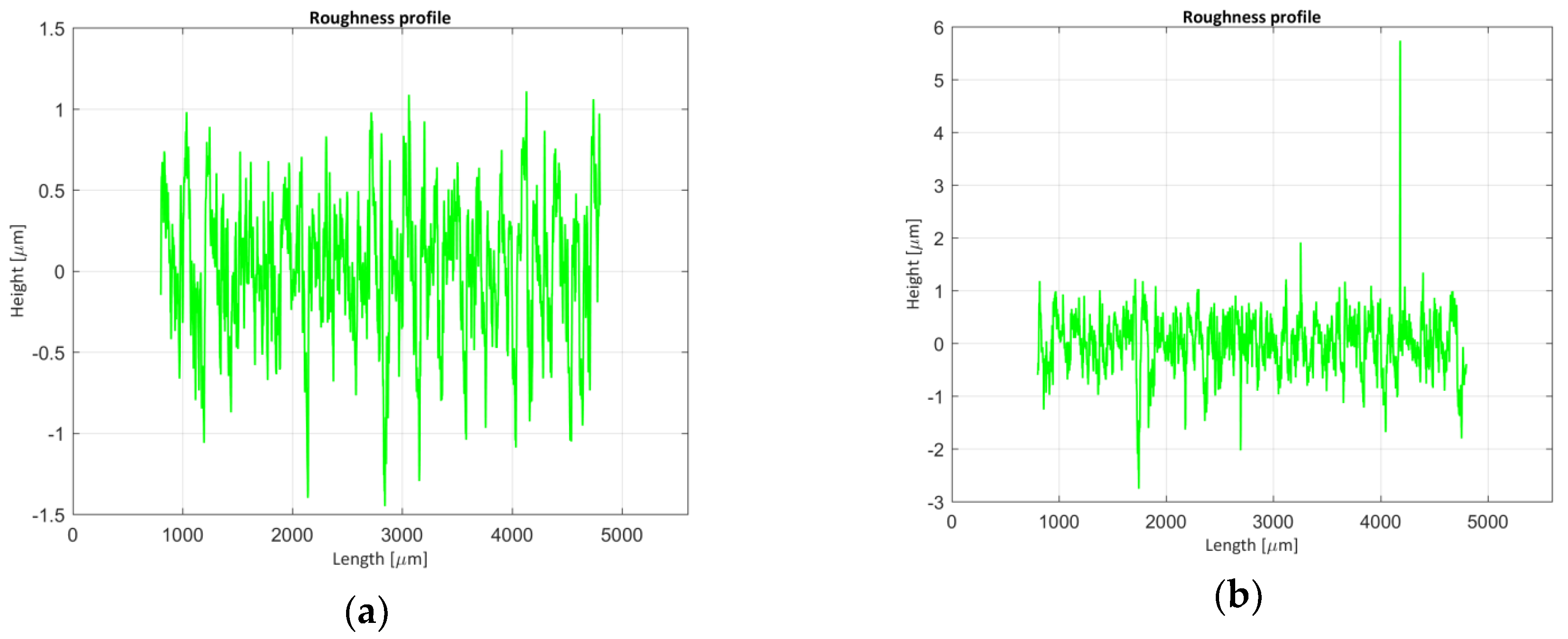
- Operational considerations: There was a significant probability of obtaining outliers or points not measured in the sample, so it was necessary to repeat the measurement a high number of times. Unmeasured points appeared when the Charge-Coupled Device (CCD) sensor of the confocal microscope did not receive enough light intensity to detect a peak position. This fact could be caused by local slope effects, which meant that the reflected light was not picked up by the target, or that the light intensity selected for the measurement was not adequate (low). On the contrary, if the luminous intensity of the equipment was very high, the CCD sensor could became saturated, tampering the peak position, and obtaining incorrect z-coordinate values. These effects could produce sharp peaks and valleys which were not real, as Figure 5b shows. Also, due to the geometry of the roughness profile, the illumination beam could only solve slopes with a maximum angle of 90 degrees.Very fine adjustment of the light intensity used in the measurement, and even the creation of different levels of illumination according to the depth of the sample, were therefore necessary. [37]. Likewise, it was be necessary to correct the unmeasured points and outliers by using interpolation and filtering techniques, respectively.
- Environmental considerations: The equipment was installed in the Laboratorio de Investigación de Materiales de Interés Tecnológico (LIMIT) laboratory of ETS de Ingeniería y Diseño Industrial (ETSIDI). The measurements were carried out at a controlled temperature of 20 ± 1 °C.
- Measurand preparation: The same as in the tactile instrument.
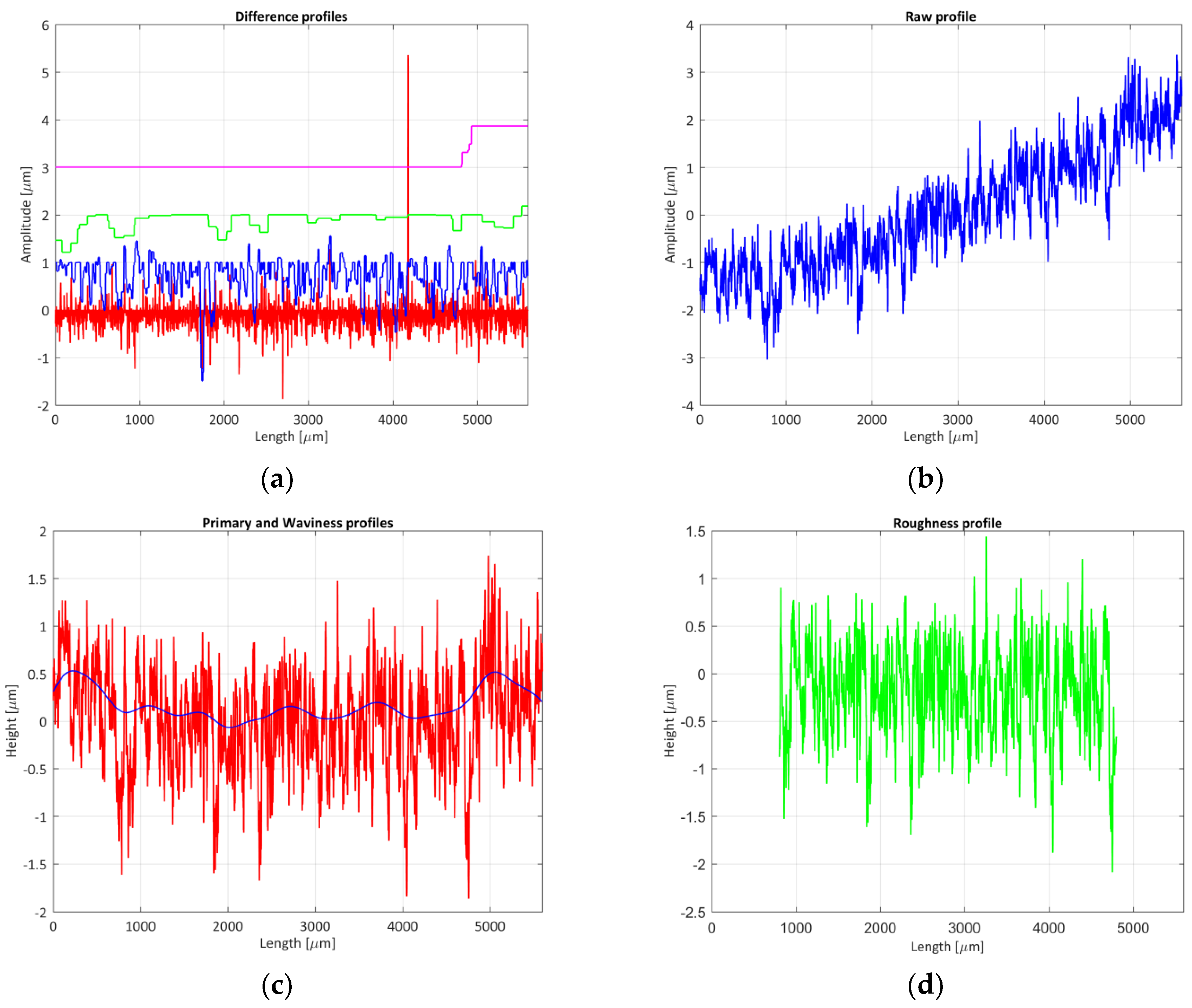
- Numeric values of the parameters: Table 6 (columns 6 and 7) and Table 7 (columns 6 to 9) show the roughness parameters obtained when evaluating measurands 8 and 2 respectively. If the results are compared when measuring the same sample with the stylus profilometers (Section 4.1), there are discrepancies between both methods, due to the causes mentioned above (outliers and not-measured points). When the standard was measured, differences of values of the parameters of between 2% and 15% were obtained. These differences could reach 300% when the piece was measured. In both cases, the smallest differences between the roughness parameter were obtained when the amplitude parameter (average of ordinates) was compared. As other authors have verified, most of the roughness parameters measured with the confocal microscope show higher values than those obtained with the profilometers. The uncertainty of the parameters showed the same order the magnitude as those obtained with the tactile instruments. To solve the problem of discrepancies, a morphological profile filter was employed: scale space techniques according to ISO 16610-49:2015 [38] so that it was possible to smooth the profile using different circular disks [39] and the outliers would be eliminated. Figure 6a,b show the results obtained when applying this technique. Also, it was decided to use a robust Gaussian regression filter [39,40] in order to improve the results, defined in standard ISO 16610-31:2016 [41]. This way, the waviness profile would not be affected by possible outliers that were not eliminated in the previous step. Figure 6c shows the primary profile and the waviness profile, and Figure 6d shows the roughness profile. By applying these modifications, it was possible to observe how the results obtained improve considerably when implementing the previous techniques, Table 6 (column 9), obtaining a maximum difference, when the Rsk parameters evaluated at 50% of its value (without the filtering technique the difference was 240%). As an average value, the difference between parameters was 14% and 105% without the filtering technique.
- Data storage requirements: The data file had 16,885 points with coordinates and a size of 310 kB.
- Cost of instrumentation/maintenance: The acquisition cost of the equipment was approximately 120,000 €. Maintenance was practically non-existent (replacement of LED light sources after about 10,000 h of operation).
5. Conclusions
Author Contributions
Funding
Conflicts of Interest
References
- Leach, R. Chapter 1: Introduction to Surface Topography. In Characterisation of Areal Surface Texture; Leach, R., Ed.; Springer: Berlin/Heidelberg, Germany, 2013; pp. 1–13. ISBN 978-3-642-36458-7. [Google Scholar]
- Leach, R.; Weckenmann, A.; Coupland, J.; Hartmann, W. Interpreting the probe-surface interaction of surface measuring instruments, or what is a surface? Surf. Topogr. Metrol. Prop. 2014, 2, 035001. [Google Scholar] [CrossRef]
- Mathiaa, T.G.; Pawlus, P.; Wieczorowski, M. Recent trends in surface metrology. Wear 2011, 271, 494–508. [Google Scholar] [CrossRef]
- Leach, R. Optical Measurement of Surface Topography; Leach, R., Ed.; Springer: Berlin/Heidelberg, Germany, 2011; ISBN 978-3-642-12011-4. [Google Scholar]
- Conroy, M.; Armstrong, J. A comparison of surface metrology techniques. J. Phys. Conf. Ser. 2005, 13, 458–465. [Google Scholar] [CrossRef]
- Artigas, R. Chaper 11: Imaging Confocal Microscopy. In Optical Measurement of Surface Topography; Leach, R., Ed.; Springer: Berlin/Heidelberg, Germany, 2011; pp. 237–286. ISBN 978-3-642-12011-4. [Google Scholar]
- Vorburger, T.V.; Rhee, H.-G.; Renegar, T.B.; Song, J.-F.; Zheng, A. Comparison of optical and stylus methods for measurement of surface texture. Int. J. Adv. Manuf. Technol. 2007, 33, 110–118. [Google Scholar] [CrossRef]
- Poon, C.Y.; Bushan, B. Comparison of surface roughness measurements by stylus profiler, AFM and non-contact optical profiler. Wear 1995, 190, 76–88. [Google Scholar] [CrossRef]
- Nouira, H.; Salgado, J.A.; El-Hayek, N.; Ducourtieux, S.; Delvallée, A.; Anwer, N. Setup of a high-precision profilometer and comparison of tactile and optical measurements of standards. Meas. Sci. Technol. 2014, 25, 044016. [Google Scholar] [CrossRef] [Green Version]
- Piska, M.; Metelkova, J. On the comparison of contact and non-contact evaluations of a machined surface. MM Sci. J. 2014, 2, 476–480. [Google Scholar] [CrossRef]
- Nieslony, P.; Krolczyk, G.M.; Zak, K.; Maruda, R.W.; Legutko, S. Comparative assessment of the mechanical and electromagnetic surfaces of explosively clad Ti-steel plates after drilling process. Precis. Eng. 2017, 47, 104–110. [Google Scholar] [CrossRef]
- Merola, M.; Ruggiero, A.; De Mattia, J.S.; Affatato, S. On the tribological behavior of retrieved hip femoral heads affected by metallic debris. A comparative investigation by stylus and optical profilometer for a new roughness measurement protocol. Measurement 2016, 90, 365–371. [Google Scholar] [CrossRef]
- Krolczyk, G.M.; Maruda, R.W.; Nieslony, P.; Wieczorowski, M. Surface morphology analysis of Duplex Stainless Steel (DSS) in Clean Production using the Power Spectral Density. Mesurement 2016, 94, 464–470. [Google Scholar] [CrossRef]
- Krolczyk, G.M.; Maruda, R.W.; Krolczyk, J.B.; Nieslony, P.; Wojciechowski, S.; Legutko, S. Parametric and nonparametric description of the surface topography in the dry and MQCL cutting conditions. Mesurement 2018, 121, 225–239. [Google Scholar] [CrossRef]
- Niemczewska-Wójcik, M. The influence of the surface geometric structure on the functionality of implants. Wear 2011, 271, 596–603. [Google Scholar] [CrossRef]
- Thompson, A.; Senin, N.; Giusca, C.; Leach, R. Topography of selectively laser melted surfaces: A comparison of different measurement methods. CIRP Ann.-Manuf. Technol. 2017, 66, 543–546. [Google Scholar] [CrossRef]
- Feidenhans’l, N.A.; Hansen, P.E.; Pilný, L.; Madsen, M.H.; Bissacco, G.; Petersen, J.C.; Taboryski, R. Comparison of optical methods for surface roughness characterization. Meas. Sci. Technol. 2015, 26, 085208. [Google Scholar] [CrossRef] [Green Version]
- ISO 16610-21:2011. Geometrical Product Specifications (GPS)—Filtration—Part 21: Linear Profile Filters: Gaussian Filters; ISO: Geneva, Switzerland, 2011. [Google Scholar]
- ISO 4287:1997. Geometrical Product Specifications (GPS)—Surface Texture: Profile Method—Terms, Definitions and Surface Texture Parameters; ISO: Geneva, Switzerland, 1997. [Google Scholar]
- ISO 4288:1996. Geometrical Product Specifications (GPS)—Surface Texture: Profile Method—Rules and Procedures for the Assessment of Surface Texture; ISO: Geneva, Switzerland, 1996. [Google Scholar]
- Cox, M.G.; Siebert, B.R.L. The use of a Monte Carlo method for evaluating uncertainty and expanded uncertainty. Metrologia 2006, 43, S178–S188. [Google Scholar] [CrossRef]
- Sousa, J.A.; Ribeiro, A.S. The choice of method to the evaluation of measurement uncertainty in metrology. In Proceedings of the IMEKO XIX World Congress—Fundamental and Applied Metrology, Lisbon, Portugal, 6–11 September 2009; pp. 2388–2393. [Google Scholar]
- Caja, J.; Gómez, E.; Maresca, P. Optical measuring equipments. Part I: Calibration model and uncertainty estimation. Precis. Eng. 2015, 40, 298–304. [Google Scholar] [CrossRef]
- Evaluation of Measurement Data—Supplement 1 to the ‘Guide to the Expression of Uncertainty in Measurement’—Propagation of Distributions Using a Monte Carlo Method. Available online: https://www.bipm.org/utils/common/documents/jcgm/JCGM_101_2008_E.pdf (accessed on 19 August 2018).
- Evaluation of Measurement Data—Supplement 2 to the ‘Guide to the Expression of Uncertainty in Measurement’—Extension to Any Number of Output Quantities. Available online: https://www.bipm.org/utils/common/documents/jcgm/JCGM_102_2011_E.pdf (accessed on 19 August 2018).
- NIST Surface Roughness and Step Height Calibrations. Available online: https://www.nist.gov/sites/default/files/documents/pml/div683/grp02/nistsurfcalib.pdf (accessed on 28 June 2018).
- Harris, P.M.; Leach, R.K.; Giusca, C. Uncertainty Evaluation for the Calculation of a Surface Texture Parameter in the Profile Case; NPL Report MS 8; Queen’s Printer: Cambridge, UK, 2010; ISSN 1754-2960. [Google Scholar]
- Haitjema, H.; van Dorp, B.; Morel, M.; Schellekens, P.H.J. Uncertainty estimation by the concept of virtual instruments. In Proceedings of the Recent Developments in Traceable Dimensional Measurements, Munich, Germany, 20–21 June 2001; Decker, J.E., Ed.; SPIE: Bellingham, WA, USA, 2001; pp. 147–157. [Google Scholar]
- Internet Based Surface Metrology Algorithm Testing System. Available online: https://physics.nist.gov/VSC/jsp/index.jsp (accessed on 26 June 2018).
- Hüser, D.; Hüser, J.; Rief, S.; Seewig, J.; Thomsen-Schmidt, P. Procedure to Approximately Estimate the Uncertainty of Material Ratio Parameters due to Inhomogeneity of Surface Roughness. Meas. Sci. Technol. 2016, 27, 085005. [Google Scholar] [CrossRef]
- International Vocabulary of Metrology—Basic and General Concepts and Associated Terms (VIM). Available online: https://www.bipm.org/utils/common/documents/jcgm/JCGM_200_2012.pdf (accessed on 19 August 2018).
- Fotowicz, P. An analytical method for calculating a coverage interval. Metrologia 2006, 43, 087001. [Google Scholar] [CrossRef]
- Wübbeler, G.; Krystek, M.; Elster, C. Evaluation of measurement uncertainty and its numerical calculation by a Monte Carlo method. Meas. Sci. Technol. 2008, 19, 084009. [Google Scholar] [CrossRef]
- Cox, M.G.; Harris, P.M. The design and use of reference data sets for testing scientific software. Anal. Chim. Acta 1998, 380, 339–352. [Google Scholar] [CrossRef]
- ISO 5436-2:2012. Geometrical Product Specifications (GPS)—Surface Texture: Profile Method; Measurement Standards—Part 2: Software Measurement Standards; ISO: Geneva, Switzerland, 2012. [Google Scholar]
- RPTB Version 2.09—Software to Analyse Roughness of Profiles. Available online: https://www.ptb.de/rptb/login (accessed on 26 June 2018).
- Barajas, C. Caracterización geométrica de huellas de dureza Brinell mediante equipos ópticos. Modelo de microscopia confocal. Ph.D. Thesis, Technical University of Madrid, Madrid, Spain, December 2015. [Google Scholar]
- ISO 16610-49:2015. Geometrical Product Specifications (GPS)—Filtration—Part 49: Morphological Profile Filters: Scale Space Techniques; ISO: Geneva, Switzerland, 2015. [Google Scholar]
- Muralikrishnan, B.; Raja, J. Computational Surface and Roundness Metrology; Springer: London, UK, 2009; pp. 1–263. ISBN 978-1-84800-296-8. [Google Scholar]
- Hüser, D. Selected Filtration Methods of the Standard ISO 16610, 5 Precision Engineering, PTB. 2016. Available online: https://www.ptb.de/cms/fileadmin/internet/fachabteilungen/abteilung_5/5.1_oberflaechenmesstechnik/DKD-Richtlinien/Selected_Filtration_Methods_of_ISO-16610.pdf (accessed on 26 June 2018).
- ISO 16610-31:2016. Geometrical Product Specifications (GPS)—Filtration—Part 31: Robust Profile Filters: Gaussian Regression Filters; ISO: Geneva, Switzerland, 2016. [Google Scholar]


| Parameter | Reference Value | Calculated Value | Q1 (×10−6) | Percentage Difference (%) |
|---|---|---|---|---|
| Rt [μm] | 1.09408 | 1.09408 | 1.5 | 0.0001 |
| Rz [μm] | 0.89833 | 0.89833 | 1.9 | 0.0002 |
| Rp [μm] | 0.46672 | 0.46672 | 4.0 | 0.0008 |
| Rv [μm] | 0.43161 | 0.43161 | 2.0 | 0.0005 |
| Ra [μm] | 0.16764 | 0.16765 | 10.3 | 0.0061 |
| Rq [μm] | 0.20479 | 0.20479 | 2.2 | 0.0011 |
| Rsk [-] | 0.1388 | 0.1388 | 3.5 | 0.0025 |
| Rku [-] | 2.37947 | 2.37947 | 6.6 | 0.0027 |
| RSm [μm] | 255.82 | 255.83 | 6542.4 | 0.0025 |
| Parameter | PTB Reference Value | Calculated Value | Q1 (×10−3) | Percentage Difference (%) |
|---|---|---|---|---|
| Rt [μm] | 2.0468 | 2.0489 | 2.1 | 0.1026 |
| Rz [μm] | 2.0037 | 2.0051 | 1.4 | 0.0699 |
| Rp [μm] | 1.0109 | 1.0116 | 0.7 | 0.0692 |
| Rv [μm] | 0.9928 | 0.9935 | 0.7 | 0.0705 |
| Ra [μm] | 0.8943 | 0.8947 | 0.4 | 0.0447 |
| Rq [μm] | 0.9068 | 0.9071 | 0.3 | 0.0331 |
| Rsk [-] | 0.0107 | 0.0110 | 0.3 | 2.8037 |
| Rku [-] | 1.0516 | 1.0511 | 0.5 | −0.0475 |
| RSm [μm] | 80.96 | 80.89 | 70 | −0.0865 |
| Instrument | Standard Deviation Rp (μm) | Standard Deviation Rv (μm) |
|---|---|---|
| SP-1 | 0.0685 | 0.0584 |
| SP-2 | 0.0539 | 0.0747 |
| CM-3 | 0.0545 | 0.0707 |
| Roughness Parameter | Parameter Estimation y | Standard Uncertainty u(y) | Shortest 95% Coverage Interval | |
|---|---|---|---|---|
| Lower Limit | Upper Limit | |||
| Rt [μm] | 3.433 | 0.032 | 3.375 | 3.496 |
| Rz [μm] | 3.367 | 0.016 | 3.336 | 3.399 |
| Rp [μm] | 1.679 | 0.012 | 1.658 | 1.703 |
| Rv [μm] | 1.688 | 0.012 | 1.667 | 1.711 |
| Ra [μm] | 0.9977 | 0.0009 | 0.9960 | 0.9993 |
| Rq [μm] | 1.1062 | 0.0009 | 1.1045 | 1.1080 |
| Rsk [-] | 0.0019 | 0.0016 | −0.0012 | 0.0052 |
| Rku [-] | 1.4860 | 0.0015 | 1.4829 | 1.4888 |
| RSm [μm] | 100.167 | 0.018 | 100.142 | 100.206 |
| Roughness Parameter | Rt | Rz | Rp | Rv | Ra | Rq | Rsk | Rku | RSm |
|---|---|---|---|---|---|---|---|---|---|
| Rt | 1.00 | 0.72 | 0.51 | 0.51 | 0.08 | 0.11 | −0.01 | 0.14 | 0.00 |
| Rz | 0.72 | 1.00 | 0.71 | 0.71 | 0.12 | 0.17 | −0.01 | 0.22 | −0.01 |
| Rp | 0.51 | 0.71 | 1.00 | 0.00 | 0.09 | 0.12 | 0.12 | 0.14 | −0.02 |
| Rv | 0.51 | 0.71 | 0.00 | 1.00 | 0.08 | 0.12 | −0.14 | 0.17 | 0.00 |
| Ra | 0.08 | 0.12 | 0.09 | 0.08 | 1.00 | 0.91 | 0.00 | −0.29 | −0.04 |
| Rq | 0.11 | 0.17 | 0.12 | 0.12 | 0.91 | 1.00 | 0.01 | 0.01 | −0.03 |
| Rsk | −0.01 | −0.01 | 0.12 | −0.14 | 0.00 | 0.01 | 1.00 | −0.01 | −0.01 |
| Rku | 0.14 | 0.22 | 0.14 | 0.17 | −0.29 | 0.01 | −0.01 | 1.00 | 0.01 |
| RSm | 0.00 | −0.01 | −0.02 | 0.00 | −0.04 | −0.03 | −0.01 | 0.01 | 1.00 |
| Instrument | SP-1 | SP-2 | CM-3 | |||
|---|---|---|---|---|---|---|
| Parameter Estimation | Standard Uncertainty | Parameter Estimation | Standard Uncertainty | Parameter Estimation | Standard Uncertainty | |
| Rt [μm] | 3.433 | 0.032 | 4.015 | 0.074 | 3.831 | 0.034 |
| Rz [μm] | 3.367 | 0.016 | 3.781 | 0.036 | 3.686 | 0.017 |
| Rp [μm] | 1.679 | 0.012 | 1.866 | 0.025 | 1.947 | 0.012 |
| Rv [μm] | 1.688 | 0.012 | 1.915 | 0.026 | 1.739 | 0.011 |
| Ra [μm] | 0.9977 | 0.0009 | 1.0189 | 0.0019 | 1.0180 | 0.0007 |
| Rq [μm] | 1.1062 | 0.0009 | 1.1370 | 0.0020 | 1.1309 | 0.0007 |
| Rsk [-] | 0.0019 | 0.0016 | −0.0455 | 0.0039 | 0.0406 | 0.0013 |
| Rku [-] | 1.4860 | 0.0015 | 1.4828 | 0.0044 | 1.5104 | 0.0012 |
| RSm [μm] | 100.167 | 0.018 | 103.3108 | 0.027 | 101.808 | 0.017 |
| Instrument | SP-1 | SP-2 | CM-3 (With Outliers) | CM-3 (Outliers Removed) | ||||
|---|---|---|---|---|---|---|---|---|
| Parameter Estimation | Standard Uncertainty | Parameter Estimation | Standard Uncertainty | Parameter Estimation | Standard Uncertainty | Parameter Estimation | Standard Uncertainty | |
| Rt [μm] | 2.613 | 0.046 | 2.939 | 0.088 | 8.484 | 0.044 | 3.442 | 0.090 |
| Rz [μm] | 2.243 | 0.022 | 2.350 | 0.038 | 4.061 | 0.019 | 2.632 | 0.029 |
| Rp [μm] | 1.010 | 0.016 | 1.064 | 0.027 | 2.250 | 0.014 | 1.295 | 0.018 |
| Rv [μm] | 1.233 | 0.016 | 1.286 | 0.027 | 1.811 | 0.014 | 1.337 | 0.023 |
| Ra [μm] | 0.3300 | 0.0008 | 0.3697 | 0.0018 | 0.39844 | 0.00063 | 0.3732 | 0.0018 |
| Rq [μm] | 0.4186 | 0.0008 | 0.4661 | 0.0019 | 0.53093 | 0.00065 | 0.4660 | 0.0011 |
| Rsk [-] | −0.2420 | 0.0084 | −0.4338 | 0.0168 | 0.338 | 0.012 | −0.375 | 0.010 |
| Rku [-] | 3.0868 | 0.0191 | 3.0862 | 0.0415 | 12.79 | 0.13 | 3.107 | 0.027 |
© 2018 by the authors. Licensee MDPI, Basel, Switzerland. This article is an open access article distributed under the terms and conditions of the Creative Commons Attribution (CC BY) license (http://creativecommons.org/licenses/by/4.0/).
Share and Cite
Caja García, J.; Sanz Lobera, A.; Maresca, P.; Fernández Pareja, T.; Wang, C. Some Considerations about the Use of Contact and Confocal Microscopy Methods in Surface Texture Measurement. Materials 2018, 11, 1484. https://doi.org/10.3390/ma11081484
Caja García J, Sanz Lobera A, Maresca P, Fernández Pareja T, Wang C. Some Considerations about the Use of Contact and Confocal Microscopy Methods in Surface Texture Measurement. Materials. 2018; 11(8):1484. https://doi.org/10.3390/ma11081484
Chicago/Turabian StyleCaja García, Jesús, Alfredo Sanz Lobera, Piera Maresca, Teresa Fernández Pareja, and Chen Wang. 2018. "Some Considerations about the Use of Contact and Confocal Microscopy Methods in Surface Texture Measurement" Materials 11, no. 8: 1484. https://doi.org/10.3390/ma11081484