Transient Thermal Stress Problem of a Functionally Graded Magneto-Electro-Thermoelastic Hollow Sphere

Abstract

This article is concerned with the theoretical analysis of the functionally graded magneto-electro-thermoelastic hollow sphere due to uniform surface heating. We analyze the transient thermoelastic problem for a functionally graded hollow sphere constructed of the spherical isotropic and linear magneto-electro-thermoelastic materials using a laminated composite mode as one of theoretical approximation in the spherically symmetric state. As an illustration, we carry out numerical calculations for a functionally graded hollow sphere constructed of piezoelectric and magnetostrictive materials and examine the behaviors in the transient state. The effects of the nonhomogeneity of material on the stresses, electric potential, and magnetic potential are investigated.

1. Introduction

Functionally graded materials (FGMs) are new nonhomogeneous material systems that two or more different material ingredients changes continuously and gradually. The concept of FGMs is applicable to many industrial fields such as aerospace, nuclear energy, chemical plant, electronics and so on. On the other hand, it has recently been found that composites made of piezoelectric and magnetostrictive materials exhibit the magnetoelectric effect, which is not seen in piezoelectric or magnetostrictive materials [1]. These materials are known as multiferroic composites [2]. These composites exhibit a coupling among magnetic, electric, and elastic fields. In the past, various problems in magneto-electro-elastic media that exhibit anisotropic and linear coupling among the magnetic, electric, and elastic fields were analyzed. Examples for the plates and beams were analyzed in the papers [3,4,5]. Examples for the shell type structures were analyzed in the papers [6,7,8]. Examples of functionally graded magneto-electro-elastic media are as follows. Wang and Ding [9] treated spherically symmetric transient responses of a functionally graded magneto-electro-elastic hollow sphere. Ma and Lee [10] analyzed an in-plane problem in functionally graded magneto-electro-elastic bimaterials. Yu and Wu [11] analyzed the propagation of circumferential wave in magneto-electro-elastic functionally graded cylindrical curved plates. Wu and Lu [12] analyzed the 3D dynamics responses of functionally graded magneto-electro-elastic plates. Huang et al. [13] analyzed the static problem of an anisotropic functionally graded magneto-electro-elastic beams subjected to arbitrary loading. Lee and Ma [14] analyzed the two-dimensional problem of two bonded dissimilar half-planes for functionally graded magnetoelectroelastic materials subjected to generalized line forces and screw dislocations.

Examples of the thermal stress problems of electro-magneto-elastic media are as follows, Ganesan et al. [15] analyzed the response of a layered, multiphase magnetoelectroelastic cylinder subjected to an axisymmetric temperature distribution using finite element procedures. Kumaravel et al. [16] analyzed the response of a three-layered magnetoelectroelastic strip subjected to uniform temperature rise and non-uniform temperature distribution using finite element procedures. Hou et al. [17] obtained 2D fundamental solutions of a steady point heat source in infinite and semi-infinite orthotropic electro-magneto-thermo-elastic planes. With regard to transient thermal stress problems of electro-magneto-elastic media, Wang and Niraula [18] analyzed transient thermal fracture in transversely isotropic electro-magneto-elastic cylinders. The exact solution of a transient analysis of multilayered magneto-electro-thermoelastic strip subjected to nonuniform heat supply was obtained in the paper [19]. The exact solution of a transient analysis of multilayered magneto-electro-thermoelastic hollow cylinder subjected to uniform heat supply was obtained in the paper [20]. Though a several transient thermal stress problems of the functionally graded hollow spheres [21,22] using a laminated composite model were analyzed already, theses studies don’t consider a coupling among magnetic, electric, and thermoelastic fields. However, to the author’s knowledge, the transient thermal stress problem for a functionally graded magneto-electro-thermoelastic hollow spheres under unsteady heat supply considering a coupling among magnetic, electric, and thermoelastic fields has not been reported.

In the present article, we have analyzed the transient behavior of a functionally graded magneto-electro-thermoelastic hollow sphere due to uniform surface heating. We assumed that the magneto-electro-thermoelastic materials are polarized and magnetized in the radial direction. We analyze the transient thermal stress problem for a functionally graded hollow sphere constructed of the spherical isotropic and linear magneto-electro-thermoelastic materials using a laminated composite model as one of theoretical approximation. We carried out numerical calculations for a functionally graded hollow sphere composed of piezoelectric and magnetostrictive materials, and examined the effects of the nonhomogeneity of material on the stresses, electric potential, and magnetic potential.

2. Analysis

We consider a functionally graded hollow sphere constructed of the spherical isotropic and linear magneto-electro-thermoelastic materials. We analyze the transient thermal stress problem using a multilayered composite hollow sphere model with a number N of homogeneous layers. The hollow sphere’s inner and outer radii are designated a and b, respectively. r_i is the outer radius of the ith layer. Throughout this article, the indices i (=1,2,…,N) are associated with the ith layer of a composite hollow sphere from the inner side.

2.1. Heat Conduction Problem

We assumed that the multilayered hollow sphere is initially at zero temperature and its inner and outer surfaces are suddenly heated by surrounding media having constant temperatures T_a and T_b with relative heat transfer coefficients h_a and h_b, respectively. Then, the temperature distribution is one-dimensional, and the transient heat conduction equation for the ith layer is written in the following form:

$$\frac{\partial {\overline{T}}_i}{\partial \tau }={\overline{\kappa }}_{ri}(\frac{{\partial }^2{\overline{T}}_i}{\partial {\overline{r}}^2}+\frac{2}{\overline{r}}\frac{\partial {\overline{T}}_i}{\partial \overline{r}});i=1,2,\cdots ,N$$

(1)

The initial and thermal boundary conditions in dimensionless form are

$$\tau =0;{\overline{T}}_i=0;i=1,2,\cdots ,N$$

(2)

$$\overline{r}=\overline{a};\frac{\partial {\overline{T}}_1}{\partial \overline{r}}-H_a{\overline{T}}_1=-H_a{\overline{T}}_a$$

(3)

$$\overline{r}=R_i;{\overline{T}}_i={\overline{T}}_{i+1};i=1,2,\cdots ,N-1$$

(4)

$$\overline{r}=R_i;{\overline{\lambda }}_{ri}\frac{\partial {\overline{T}}_i}{\partial \overline{r}}={\overline{\lambda }}_{r,i+1}\frac{\partial {\overline{T}}_{i+1}}{\partial \overline{r}};i=1,2,\cdots ,N-1$$

(5)

$$\overline{r}=1;\frac{\partial {\overline{T}}_N}{\partial \overline{r}}+H_b{\overline{T}}_N=H_b{\overline{T}}_b$$

(6)

In Equations (1)–(6), we introduced the following dimensionless values:

$$\begin{array}{c}({\overline{T}}_i,{\overline{T}}_a,{\overline{T}}_b)=(T_i,T_a,T_b)/T_0,(\overline{r},R_i,\overline{a})=(r,r_i,a)/b,\tau ={\kappa }_{0}t/b^2\\ {\overline{\kappa }}_{ri}={\kappa }_{ri}/{\kappa }_0,{\overline{\lambda }}_{ri}={\lambda }_{ri}/{\lambda }_0,(H_a,H_b)=(h_a,h_b)b\end{array}$$

(7)

where T_i is the temperature change; t is time; λ_ri is the thermal conductivity in the radial direction; κ_ri is the thermal diffusivity in the radial direction; and T₀, λ₀ and κ₀ are typical values of temperature, thermal conductivity, and thermal diffusivity, respectively. To solve the fundamental equation (1), we introduced the Laplace transformation with respect to the variable τ as follows;

$${\overline{T}}_i^{*}(\overline{r},p)={\displaystyle {\int }_0^{\infty }{\overline{T}}_i(\overline{r},\tau )}{e}^{-p\tau }d\tau$$

(8)

Performing the Laplace transformation on Equation (1) under the condition of Equation (2) gives

$$\frac{d^2{\overline{T}}_i^{*}}{d{\overline{r}}^2}+\frac{2}{\overline{r}}\frac{d{\overline{T}}_i^{*}}{d\overline{r}}+{\mu }^2{\beta }_i^2{\overline{T}}_i^{*}=0$$

(9)

where

$${\mu }^2=-p,{\beta }_i=\frac{1}{\sqrt{{\overline{\kappa }}_{ri}}}$$

(10)

The general solution of Equation (9) is

$${\overline{T}}_i^{*}=A_i{j}_0({\beta }_i\mu \overline{r})+B_i{y}_0({\beta }_i\mu \overline{r})$$

(11)

where j₀() and y₀() are zeroth-order spherical Bessel functions of the first and second kind, respectively. Furthermore, A_i and B_i are unknown constants determined from the boundary conditions. Substituting Equation (11) into the boundary conditions in the transformed domain from Equations (3)–(6), these equations are represented in matrix form as follows:

$$\left[a_{kl}\right]\left\{\begin{array}{c}{A}_1\\ B_1\\ ⋮\\ A_N\\ B_N\end{array}\right\}=\frac{1}{p}\left\{c_k\right\}$$

(12)

Making use of Cramer’s formula, the constants A_i and B_i can be determined from Equation (12). Then the temperature solution in the transformed domain is

$${\overline{T}}_i^{*}=\frac{1}{p\Delta }[{\overline{A}}_i{j}_0({\beta }_i\mu \overline{r})+{\overline{B}}_i{y}_0({\beta }_i\mu \overline{r})]$$

(13)

where Δ is the determinant of 2N × 2N matrix [a_kl], and the coefficients ${\overline{A}}_i$ and ${\overline{B}}_i$ are defined as determinants of a matrix similar to the coefficient matrix [a_kl], in which the (2i − 1)th column or 2ith column is replaced with the constant vector {c_k}, respectively. Using the residue theorem, we can accomplish the inverse Laplace transformation on Equation (13). Because the single-valued poles of Equation (13) correspond to p = 0 and the roots of Δ = 0, in which the residue for p = 0 gives a solution for the steady state. Accomplishing the inverse Laplace transformation of Equation (13), the solution of Equation (1) is written as follows:

$${\overline{T}}_i=\frac{1}{F}({{\overline{A}}^{\prime }}_i+\frac{{{\overline{B}}^{\prime }}_i}{\overline{r}})+{\displaystyle \sum _{j=1}^{\infty }\frac{2\exp (-{\mu }_j^2\tau )}{{\mu }_j{\Delta }^{\prime }({\mu }_j)}}[{\overline{A}}_i{j}_0({\beta }_i{\mu }_j\overline{r})+{\overline{B}}_i{y}_0({\beta }_i{\mu }_j\overline{r})];i=1,2,\cdots ,N$$

(14)

where F ie the determinants of 2N × 2N matrix [e_kl], and the coefficients ${{\overline{A}}^{\prime }}_i$ and ${{\overline{B}}^{\prime }}_i$ are defined as determinants of a matrix similar to the coefficient matrix [e_kl], in which the (2i − 1)th column or 2ith column is replaced with the constant vector {c_k}, respectively. The nonzero elements of the coefficient matrices [a_kl] and [e_kl] and the constant vector {c_k} are given from the Equations (3)–(6). In Equation (14), ${\Delta }^{\prime }({\mu }_j)$ is

$${\Delta }^{\prime }({\mu }_j)={\frac{d\Delta }{d\mu }|}_{\mu ={\mu }_j}$$

(15)

and μ_j is the jth positive root of the following transcendental equation

$$\Delta (\mu )=0$$

(16)

2.2. Thermoelastic Problem

We developed the analysis of a multilayered magneto-electro-thermoelastic hollow sphere as a spherically symmetric state. The displacement-strain relations are expressed in dimensionless form as follows:

$${\overline{\epsilon }}_{rri}={\overline{u}}_{ri}{,}_{\overline{r}},{\overline{\epsilon }}_{\theta \theta i}={\overline{\epsilon }}_{\phi \phi i}=\frac{{\overline{u}}_{ri}}{\overline{r}},{\overline{\gamma }}_{r\theta i}={\overline{\gamma }}_{r\phi i}={\overline{\gamma }}_{\theta \phi i}=0$$

(17)

where the comma denotes partial differentiation with respect to the variable that follows. For the spherical isotropic and linear magneto-electro-thermoelastic material, the constitutive relations are expressed in dimensionless form as follows:

$$\begin{array}{c}{\overline{\sigma }}_{rri}={\overline{C}}_{11i}{\overline{\epsilon }}_{rri}+2{\overline{C}}_{12i}{\overline{\epsilon }}_{\theta \theta i}-{\overline{\beta }}_{ri}{\overline{T}}_i-{\overline{e}}_{1i}{\overline{E}}_{ri}-{\overline{q}}_{1i}{\overline{H}}_{ri}\\ {\overline{\sigma }}_{\theta \theta i}={\overline{\sigma }}_{\phi \phi i}={\overline{C}}_{12i}{\overline{\epsilon }}_{rri}+({\overline{C}}_{22i}+{\overline{C}}_{23i}){\overline{\epsilon }}_{\theta \theta i}-{\overline{\beta }}_{\theta i}{\overline{T}}_i-{\overline{e}}_{2i}{\overline{E}}_{ri}-{\overline{q}}_{2i}{\overline{H}}_{ri}\end{array}$$

(18)

where

$${\overline{\beta }}_{ri}={\overline{C}}_{11i}{\overline{\alpha }}_{ri}+2{\overline{C}}_{12i}{\overline{\alpha }}_{\theta i},{\overline{\beta }}_{ri}={\overline{C}}_{11i}{\overline{\alpha }}_{ri}+2{\overline{C}}_{12i}{\overline{\alpha }}_{\theta i}$$

(19)

The constitutive equations for the electric and the magnetic fields in dimensionless form are given as

$${\overline{D}}_{ri}={\overline{e}}_{1i}{\overline{\epsilon }}_{rri}+2{\overline{e}}_{2i}{\overline{\epsilon }}_{\theta \theta i}+{\overline{\eta }}_{1i}{\overline{E}}_{ri}+{\overline{d}}_{1i}{\overline{H}}_{ri}+{\overline{p}}_{1i}{\overline{T}}_i$$

(20)

$${\overline{B}}_{ri}={\overline{q}}_{1i}{\overline{\epsilon }}_{rri}+2{\overline{q}}_{2i}{\overline{\epsilon }}_{\theta \theta i}+{\overline{d}}_{1i}{\overline{E}}_{ri}+{\overline{\mu }}_{1i}{\overline{H}}_{ri}+{\overline{m}}_{1i}{\overline{T}}_i$$

(21)

The relation between the electric field intensity and the electric potential ${\phi }_i$ in dimensionless form is defined as

$${\overline{E}}_{ri}=-{\overline{\phi }}_i{,}_{\overline{r}}$$

(22)

The relation between the magnetic field intensity and the magnetic potential ${\psi }_i$ in dimensionless form is defined as

$${\overline{H}}_{ri}=-{\overline{\psi }}_i{,}_{\overline{r}}$$

(23)

The equilibrium equation is expressed in dimensionless form as follows:

$${\overline{\sigma }}_{rri}{,}_{\overline{r}}+\frac{2}{\overline{r}}({\overline{\sigma }}_{rri}-{\overline{\sigma }}_{\theta \theta i})=0$$

(24)

If the electric charge density is absent, the equations of electrostatics and magnetostatics are expressed in dimensionless form as follows:

$${\overline{D}}_{ri}{,}_{\overline{r}}+\frac{2{\overline{D}}_{ri}}{\overline{r}}=0$$

(25)

$${\overline{B}}_{ri}{,}_{\overline{r}}+\frac{2{\overline{B}}_{ri}}{\overline{r}}=0$$

(26)

In Equations (17)–(26), the following dimensionless values are introduced:

$$\begin{array}{c}{\overline{\sigma }}_{kli}=\frac{{\sigma }_{kli}}{{\alpha }_0{Y}_0{T}_0},({\overline{\epsilon }}_{kli},{\overline{\gamma }}_{kli})=\frac{({\epsilon }_{kli},{\gamma }_{kli})}{{\alpha }_0{T}_0},{\overline{u}}_{ri}=\frac{u_{ri}}{{\alpha }_0{T}_{0}b},{\overline{\alpha }}_{ki}=\frac{{\alpha }_{ki}}{{\alpha }_0},{\overline{C}}_{kli}=\frac{C_{kli}}{Y_0}\\ {\overline{D}}_{ri}=\frac{D_{ri}}{{\alpha }_0{Y}_0{T}_0\left|d_0\right|},{\overline{B}}_{ri}=\frac{B_{ri}\left|d_0\right|{\kappa }_0}{b{\alpha }_0{T}_0},{\overline{\phi }}_i=\frac{{\phi }_i\left|d_0\right|}{{\alpha }_0{T}_{0}b},{\overline{\psi }}_i=\frac{{\psi }_i}{\left|d_0\right|{\kappa }_0{\alpha }_0{Y}_0{T}_0},\\ {\overline{e}}_{ki}=\frac{e_{ki}}{Y_0\left|d_0\right|},{\overline{\eta }}_{1i}=\frac{{\eta }_{1i}}{Y_0{\left|d_0\right|}^2},{\overline{q}}_{ki}=\frac{q_{ki}{\kappa }_0\left|d_0\right|}{b},{\overline{\mu }}_{1i}=\frac{{\mu }_{1i}{\kappa }_0^2{\left|d_0\right|}^2{Y}_0}{b^2},\\ {\overline{d}}_{1i}=\frac{{\kappa }_0{d}_{1i}}{b},{\overline{p}}_{1i}=\frac{p_{1i}}{{\alpha }_0{Y}_0\left|d_0\right|},{\overline{m}}_{1i}=\frac{m_{1i}{\kappa }_0\left|d_0\right|}{b{\alpha }_0},{\overline{E}}_{ri}=\frac{E_{ri}\left|d_0\right|}{{\alpha }_0{T}_0},{\overline{H}}_{ri}=\frac{H_{ri}b}{\left|d_0\right|{\kappa }_0{\alpha }_0{Y}_0{T}_0}\end{array}$$

(27)

where ${\sigma }_{kli}$ are the stress components; (${\epsilon }_{kli}$, ${\gamma }_{kli}$) are the strain components; u_ri is the displacement in the r direction; α_ri are the coefficients of linear thermal expansion; C_kli are the elastic stiffness constants; D_ri is the electric displacement in the r direction; B_ri is the magnetic flux density in the r direction; e_ki are the piezoelectric coefficients; η_1i is the dielectric constant; P_1i is the pyroelectric constant; q_ki are the piezomagnetic coefficients; μ_1i is the magnetic permeability coefficient; d_1i is the magnetoelectric coefficient; m_1i is the pyromagnetic constant; and α₀, Y₀ and d₀ are typical values of the coefficient of linear thermal expansion, Young’s modulus, and piezoelectric modulus, respectively.

Substituting Equations (17), (22), and (23) into Equations (18), (20), and (21) and later into Equations (24)–(26), the governing equations of the displacement u_ri, electric potential φ_i, and magnetic potential ψ_i in the dimensionless form are written as

$$\begin{array}{c}{\overline{C}}_{11i}{\overline{u}}_{ri}{,}_{\overline{r}\overline{r}}+2{\overline{C}}_{11i}{\overline{u}}_{ri}{,}_{\overline{r}}{\overline{r}}^{-1}+2({\overline{C}}_{12i}-{\overline{C}}_{22i}-{\overline{C}}_{23i}){\overline{u}}_{ri}{\overline{r}}^{-2}+{\overline{e}}_{1i}{\overline{\phi }}_i{,}_{\overline{r}\widehat{r}}+2({\overline{e}}_{1i}-{\overline{e}}_{2i}){\overline{\phi }}_i{,}_{\overline{r}}{\overline{r}}^{-1}\\ +{\overline{q}}_{1i}{\overline{\psi }}_i{,}_{\overline{r}\overline{r}}+2({\overline{q}}_{1i}-{\overline{q}}_{2i}){\overline{\psi }}_i{,}_{\overline{r}}{\overline{r}}^{-1}=2({\overline{\beta }}_{ri}-{\overline{\beta }}_{\theta i}){\overline{T}}_i{\overline{r}}^{-1}+{\overline{\beta }}_{ri}{\overline{T}}_i{,}_{\overline{r}}\end{array}$$

(28)

$$\begin{array}{c}{\overline{e}}_{1i}{\overline{u}}_{ri}{,}_{\overline{r}\overline{r}}+2({\overline{e}}_{1i}+{\overline{e}}_{2i}){\overline{u}}_{ri}{,}_{\overline{r}}{\overline{r}}^{-1}+2{\overline{e}}_{2i}{\overline{u}}_{ri}{\overline{r}}^{-2}-{\overline{\eta }}_{1i}{\overline{\phi }}_i{,}_{\overline{r}\overline{r}}-2{\overline{\eta }}_{1i}{\overline{\phi }}_i{,}_{\overline{r}}{\overline{r}}^{-1}\\ -{\overline{d}}_{1i}{\overline{\psi }}_i{,}_{\overline{r}\widehat{r}}-2{\overline{d}}_{1i}{\overline{\psi }}_i{,}_{\overline{r}}{\overline{r}}^{-1}=-{\overline{p}}_{1i}({\overline{T}}_i{,}_{\overline{r}}+2{\overline{T}}_i{\overline{r}}^{-1})\end{array}$$

(29)

$$\begin{array}{c}{\overline{q}}_{1i}{\overline{u}}_{ri}{,}_{\overline{r}\overline{r}}+2({\overline{q}}_{1i}+{\overline{q}}_{2i}){\overline{u}}_{ri}{,}_{\overline{r}}{\overline{r}}^{-1}+2{\overline{q}}_{2i}{\overline{u}}_{ri}{\overline{r}}^{-2}-{\overline{d}}_{1i}{\overline{\phi }}_i{,}_{\overline{r}\overline{r}}-2{\overline{d}}_{1i}{\overline{\phi }}_i{,}_{\overline{r}}{\overline{r}}^{-1}\\ -{\overline{\mu }}_{1i}{\overline{\psi }}_i{,}_{\overline{r}\overline{r}}-2{\overline{\mu }}_{1i}{\overline{\psi }}_i{,}_{\overline{r}}{\overline{r}}^{-1}-{\overline{\mu }}_{1i}{\overline{\psi }}_i{,}_{\overline{r}\overline{r}}-2{\overline{\mu }}_{1i}{\overline{\psi }}_i{,}_{\overline{r}}{\overline{r}}^{-1}\end{array}$$

(30)

If the inner and outer surfaces of the multilayered magneto-electro-thermoelastic hollow sphere are traction free, and the interfaces of each adjoining layer are perfectly bonded, then the boundary conditions of inner and outer surfaces and the conditions of continuity at the interfaces can be represented as follows:

$$\begin{array}{c}\overline{r}=\overline{a};{\overline{\sigma }}_{rr1}=0\\ \overline{r}=R_i;{\overline{\sigma }}_{rri}={\overline{\sigma }}_{rr,i+1},{\overline{u}}_{ri}={\overline{u}}_{r,i+1};i=1,2,\cdots ,N-1\\ \overline{r}=1;{\overline{\sigma }}_{rrN}=0\end{array}$$

(31)

The boundary conditions in the radial direction for the electric and magnetic fields are expressed as

(32)

The solutions of Equations (28)–(30) are assumed in the following form:

$${\overline{u}}_{ri}={\overline{u}}_{rci}+{\overline{u}}_{rpi},{\overline{\phi }}_i={\overline{\phi }}_{ci}+{\overline{\phi }}_{pi},{\overline{\psi }}_i={\overline{\psi }}_{ci}+{\overline{\psi }}_{pi}$$

(33)

In Equation (33), the first term on the right-hand side gives the homogeneous solution and the second term gives the particular solution. We now consider the homogeneous solution, and introduce the following equation:

$$\overline{r}=\exp (s)$$

(34)

Changing a variable with the use of Equation (34), the homogeneous expression of Equations (28)–(30) are

$$[{\overline{D}}^2+\overline{D}-{\alpha }_i]{\overline{u}}_{rci}+[{\overline{D}}^2+\overline{D}-{\beta }_{ei}\overline{D}]{\overline{\Phi }}_{ci}+[{\overline{D}}^2+\overline{D}-{\beta }_{qi}\overline{D}]{\overline{\Psi }}_{ci}=0$$

(35)

$$[{\overline{D}}^2+\overline{D}+{\beta }_{ei}(\overline{D}+1)]{\overline{u}}_{rci}-{\gamma }_i({\overline{D}}^2+\overline{D}){\overline{\Phi }}_{ci}-{\beta }_{di}({\overline{D}}^2+\overline{D}){\overline{\Psi }}_{ci}=0$$

(36)

$$[{\overline{D}}^2+\overline{D}+{\beta }_{qi}(\overline{D}+1)]{\overline{u}}_{rci}-{\beta }_{di}({\overline{D}}^2+\overline{D}){\overline{\Phi }}_{ci}-{\delta }_i({\overline{D}}^2+\overline{D}){\overline{\Psi }}_{ci}=0$$

(37)

where

$$\overline{D}=\frac{d}{ds}$$

(38)

$$\begin{array}{c}{\overline{\Phi }}_{ci}=\frac{{\overline{e}}_{1i}}{{\overline{C}}_{11i}}{\overline{\phi }}_{ci},{\overline{\Psi }}_{ci}=\frac{{\overline{q}}_{1i}}{{\overline{C}}_{11i}}{\overline{\psi }}_{ci},{\alpha }_i=\frac{2({\overline{C}}_{22i}+{\overline{C}}_{23i}-{\overline{C}}_{12i})}{{\overline{C}}_{11i}},\\ {\beta }_{ei}=\frac{2{\overline{e}}_{2i}}{{\overline{e}}_{1i}},{\beta }_{qi}=\frac{2{\overline{q}}_{2i}}{{\overline{q}}_{1i}},{\beta }_{di}=\frac{{\overline{C}}_{11i}{\overline{d}}_{1i}}{{\overline{e}}_{1i}{\overline{q}}_{1i}},{\overline{\gamma }}_i=\frac{{\overline{C}}_{11i}{\overline{\eta }}_{1i}}{{\overline{e}}_{1i}^2},{\delta }_i=\frac{{\overline{C}}_{11i}{\overline{\mu }}_{1i}}{{\overline{q}}_{1i}^2}\end{array}$$

(39)

By eliminating ${\overline{\Phi }}_{ci}$ and ${\overline{\Psi }}_{ci}$ between Eqs. (35)-(37), we can obtain an ordinary differential equation about ${\overline{u}}_{rci}$:

$$b_{3i}\overline{D}{(\overline{D}+1)}^2{\overline{u}}_{rci}+b_{1i}(\overline{D}+1){\overline{u}}_{rci}=0$$

(40)

The solution of Equation (40) can be expressed as follows when $1-4b_{1i}/b_{3i}>0$.

$${\overline{u}}_{rci}=C_{1i}{\overline{r}}^{-1}+C_{2i}{\overline{r}}^{{\lambda }_{i2}}+C_{3i}{\overline{r}}^{{\lambda }_{i3}}$$

(41)

From Equations (36), (37) and (41), we can obtain an ordinary differential equation about ${\overline{\Psi }}_{ci}$:

$$\overline{D}{\overline{\Psi }}_{ci}+{\overline{\Psi }}_{ci}=a_{3i}{C}_{2i}{e}^{{\lambda }_{i2}s}+a_{4i}{C}_{3i}{e}^{{\lambda }_{i3}s}+C_{4i}$$

(42)

Using Equation (39), the solution of Equation (42) is

$${\overline{\psi }}_{ci}=\frac{{\overline{C}}_{11i}}{{\overline{q}}_{1i}}(C_{4i}+C_{5i}{\overline{r}}^{-1}+g_{3i}{C}_{2i}{\overline{r}}^{{\lambda }_{i2}}+g_{4i}{C}_{3i}{\overline{r}}^{{\lambda }_{i3}})$$

(43)

From Equations (36), (41) and (43), we can obtain an ordinary differential equation about ${\overline{\Phi }}_{ci}$:

$$\overline{D}{\overline{\Phi }}_{ci}+{\overline{\Phi }}_{ci}=a_{1i}{C}_{2i}{e}^{{\lambda }_{i2}s}+a_{2i}{C}_{3i}{e}^{{\lambda }_{i3}s}+C_{6i}$$

(44)

Using Equation (39), the solution of Equation (44) is

$${\overline{\phi }}_{ci}=\frac{{\overline{C}}_{11i}}{{\overline{e}}_{1i}}(C_{6i}+C_{7i}{\overline{r}}^{-1}+g_{1i}{C}_{2i}{\overline{r}}^{{\lambda }_{i2}}+g_{2i}{C}_{3i}{\overline{r}}^{{\lambda }_{i3}})$$

(45)

In Equations (41)–(45)

$$\begin{array}{c}{\lambda }_{i2},{\lambda }_{i3}=\frac{-1\pm \sqrt{1-4b_{1i}/b_{3i}}}{2},\\ b_{1i}=-[{\alpha }_i{\gamma }_i+{\beta }_{ei}^2-{\beta }_{ei}-\frac{{\beta }_{qi}{\gamma }_i-{\beta }_{ei}{\beta }_{di}}{{\delta }_i{\gamma }_i-{\beta }_{di}^2}({\gamma }_i-{\beta }_{di}-{\beta }_{qi}{\gamma }_i+{\beta }_{ei}{\beta }_{di})]\\ b_{3i}=1+{\gamma }_i+\frac{{({\gamma }_i-{\beta }_{di})}^2}{{\delta }_i{\gamma }_i-{\beta }_{di}^2}\\ g_{1i}=\frac{a_{1i}}{{\lambda }_{i2}+1},g_{2i}=\frac{a_{2i}}{{\lambda }_{i3}+1},g_{3i}=\frac{a_{3i}}{{\lambda }_{i2}+1},g_{4i}=\frac{a_{4i}}{{\lambda }_{i3}+1},\\ a_{1i}=\frac{1}{{\gamma }_i{\lambda }_{i2}}[{\lambda }_{i2}^2+{\lambda }_{i2}+{\beta }_{ei}({\lambda }_{i2}+1)-{\beta }_{di}{\lambda }_{i2}{a}_{3i}]\\ a_{2i}=\frac{1}{{\gamma }_i{\lambda }_{i3}}[{\lambda }_{i3}^2+{\lambda }_{i3}+{\beta }_{ei}({\lambda }_{i3}+1)-{\beta }_{di}{\lambda }_{i3}{a}_{4i}]\\ a_{3i}=\frac{{\lambda }_{i2}+1}{{\lambda }_{i2}({\delta }_i{\gamma }_i-{\beta }_{di}^2)}[({\gamma }_i-{\beta }_{di}){\lambda }_{i2}+{\beta }_{qi}{\gamma }_i-{\beta }_{ei}{\beta }_{di}]\\ a_{4i}=\frac{{\lambda }_{i3}+1}{{\lambda }_{i3}({\delta }_i{\gamma }_i-{\beta }_{di}^2)}[({\gamma }_i-{\beta }_{di}){\lambda }_{i3}+{\beta }_{qi}{\gamma }_i-{\beta }_{ei}{\beta }_{di}]\end{array}$$

(46)

In Equations (41), (43) and (45), C_ki ($k=1,2,\cdots ,7$) are unknown constants. We have the following relation.

$$-{\alpha }_i{C}_{1i}+{\beta }_{ei}{C}_{7i}+{\beta }_{qi}{C}_{5i}=0$$

(47)

The homogeneous solutions when $1-4b_{1i}/b_{3i}\le 0$ are omitted here for brevity.

It is difficult to obtain the particular solutions using the temperature solution of Equation (14). In order to obtain the particular solutions, series expansions of Bessel functions given in Equation (14) are used. Equation (14) can be written in the following way:

$${\overline{T}}_i(\overline{r},\tau )={\displaystyle \sum _{n=0}^{\infty }[a_{in}(\tau ){\overline{r}}^{2n}+b_{in}(\tau ){\overline{r}}^{2n-1}]}$$

(48)

where

$$\begin{array}{c}{a}_{in}(\tau )=\frac{{{\overline{A}}^{\prime }}_i}{F}{\delta }_{0n}+{\displaystyle \sum _{j=1}^{\infty }{\overline{A}}_i\frac{2\exp (-{\mu }_j^2\tau )}{{\mu }_j{\Delta }^{\prime }({\mu }_j)}}\cdot \frac{{(-1)}^n{({\beta }_i{\mu }_j)}^{2n}}{(2n+1)!},\\ b_{in}(\tau )=\frac{{{\overline{B}}^{\prime }}_i}{F}{\delta }_{0n}+{\displaystyle \sum _{j=1}^{\infty }{\overline{B}}_i\frac{2\exp (-{\mu }_j^2\tau )}{{\mu }_j{\Delta }^{\prime }({\mu }_j)}}\cdot \frac{{(-1)}^{n+1}{({\beta }_i{\mu }_j)}^{2n-1}}{(2n)!}\end{array}$$

(49)

Here, ${\delta }_{0n}$ is the Kronecker delta. The particular solutions ${\overline{u}}_{rpi}$, ${\overline{\phi }}_{ip}$, and ${\overline{\psi }}_{pi}$ are obtained as the function system like Equation (48). Then, the stress components, electric displacement, and magnetic flux density can be evaluated from Equations (41), (43) and (45). Details of the solutions are omitted from here for brevity. The unknown constants in the homogeneous solutions are determined so as to satisfy the boundary conditions in (31) and (32).

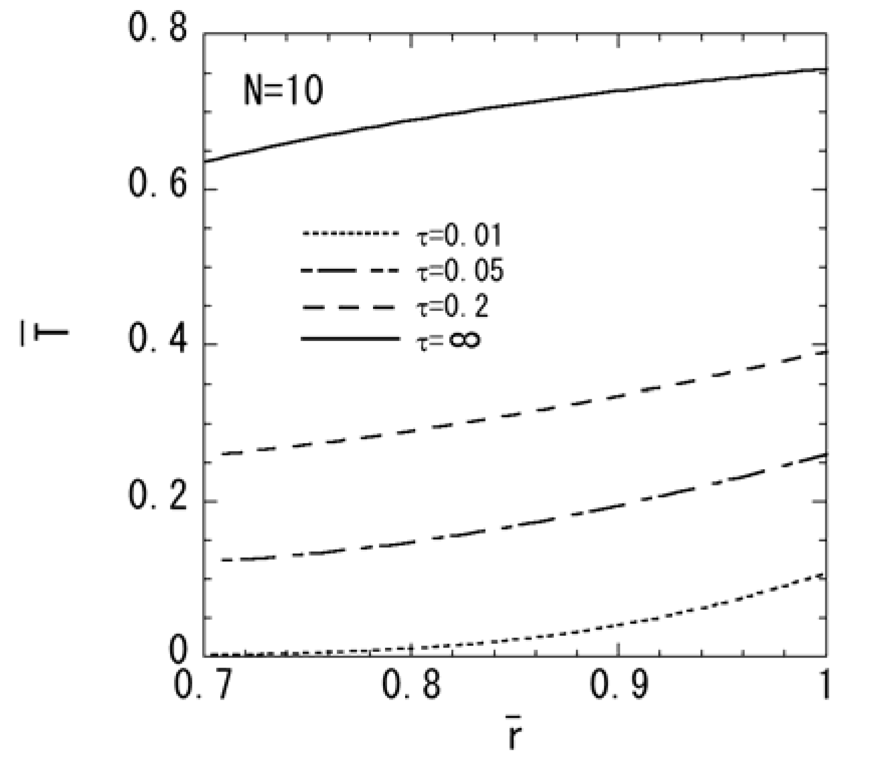
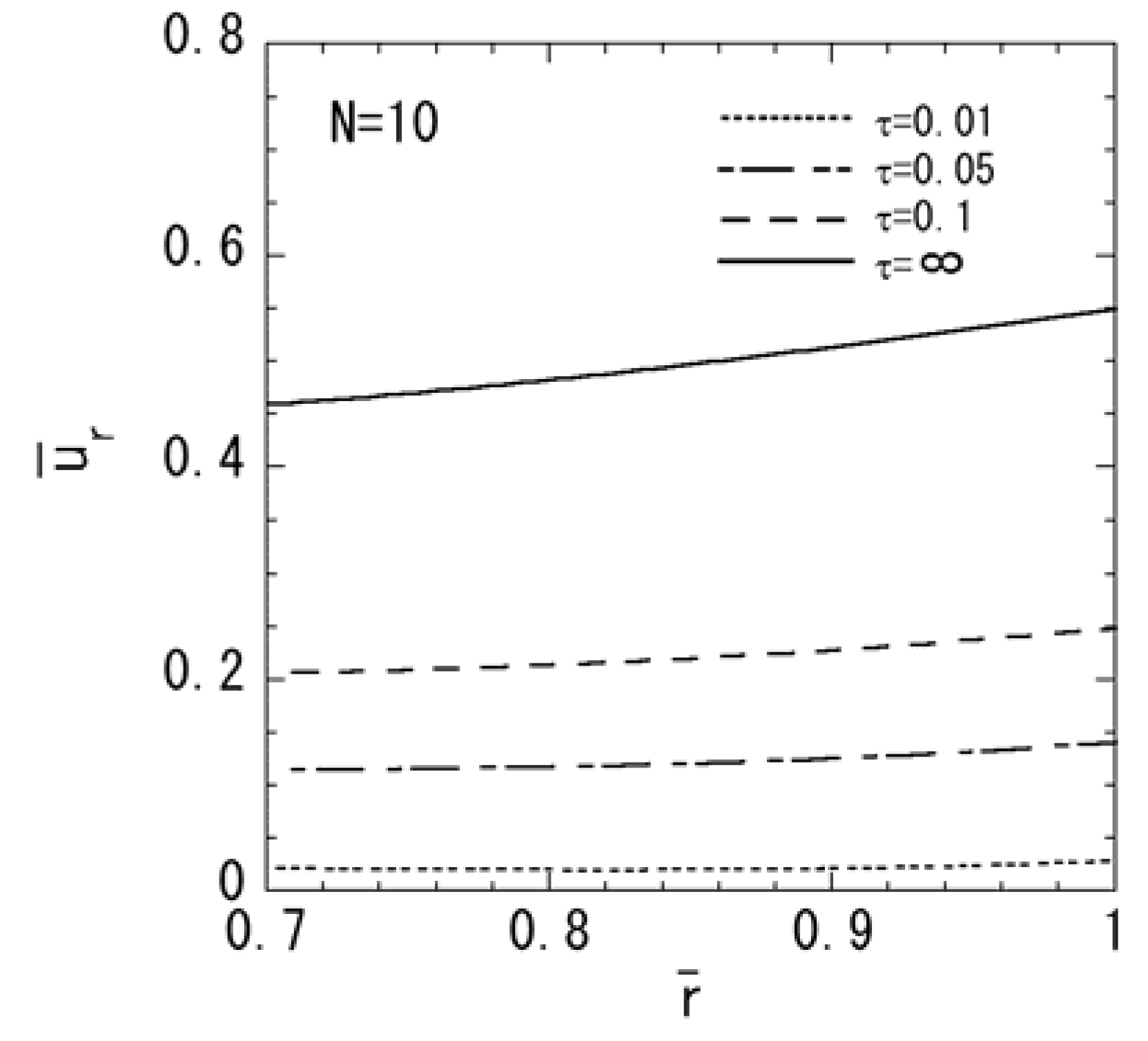
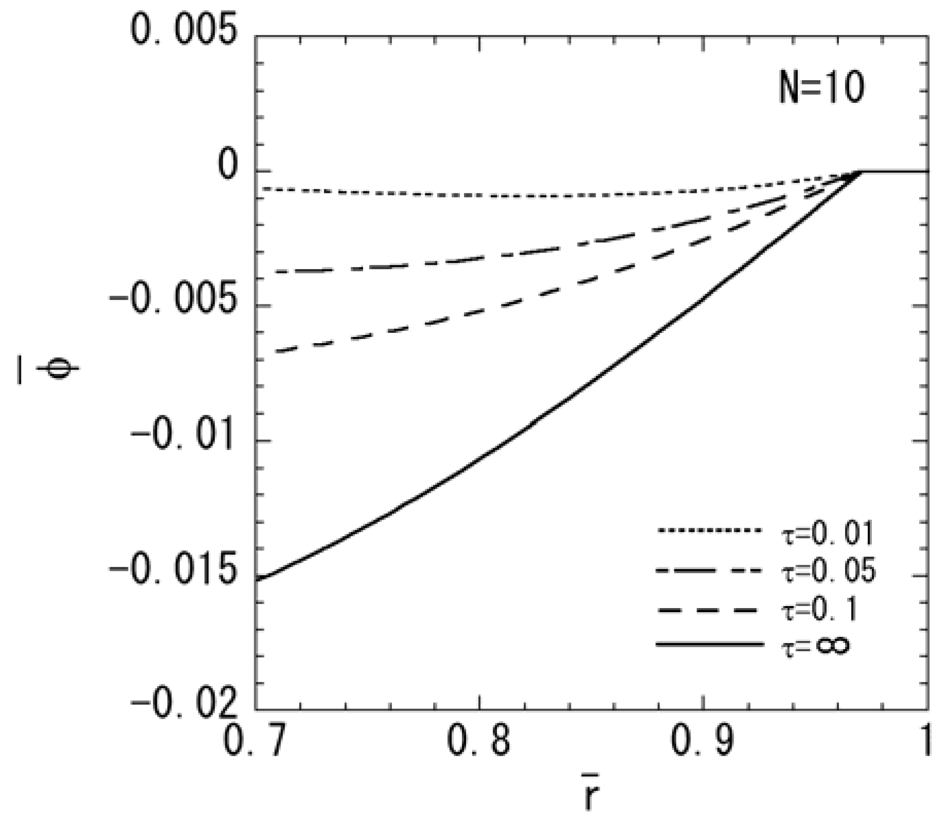
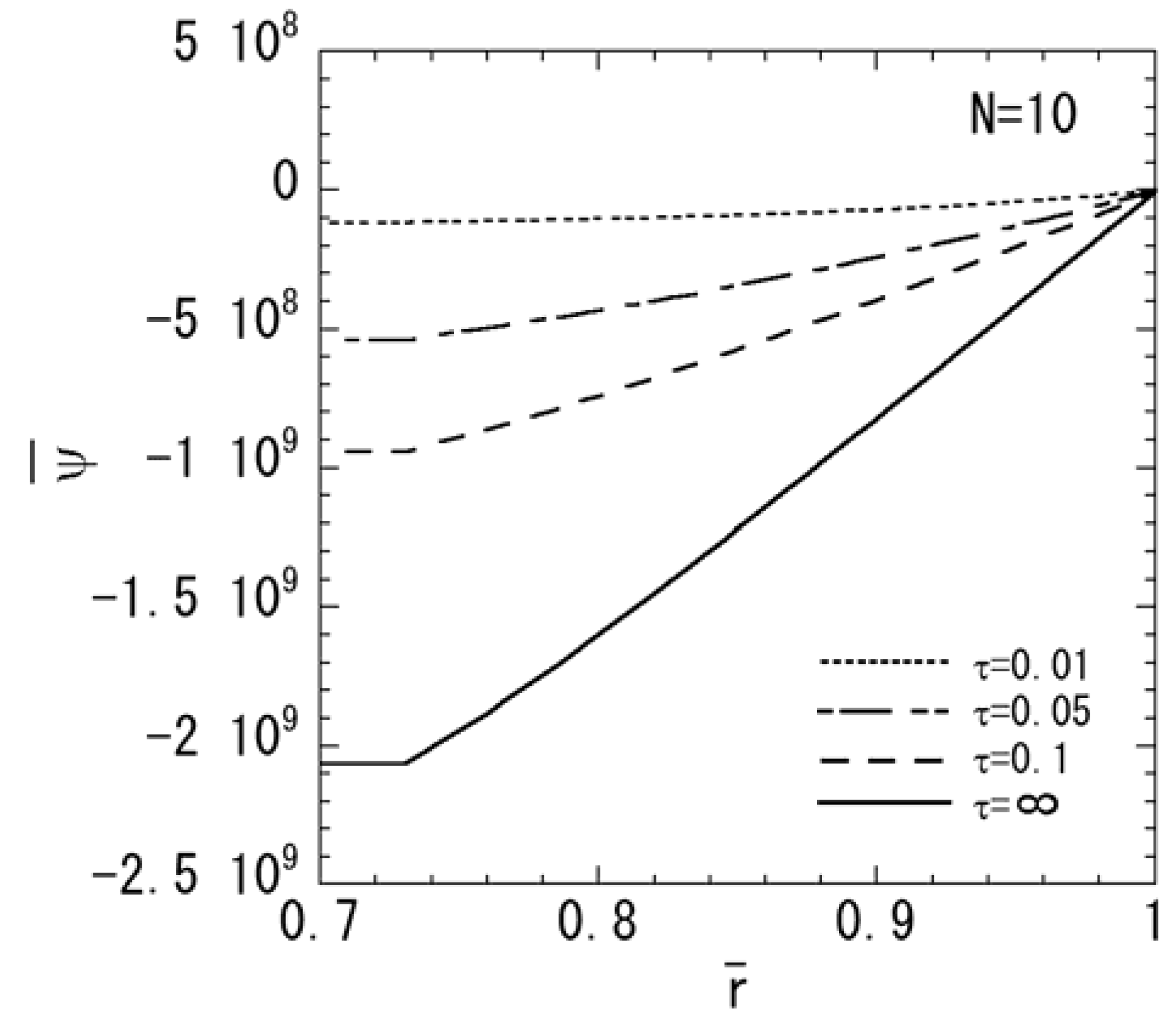
3. Numerical Results

To illustrate the foregoing analysis, we consider the functionally graded hollow sphere composed of piezoelectric and magnetostrictive materials. The piezoelectric material is made up of BaTiO₃, and the magnetostrictive material is made up of CoFe₂O₄. Numerical parameters of heat conduction and shape are presented as follows:

$$\begin{array}{c}{H}_a=H_b=1.0,{\overline{T}}_a=0,{\overline{T}}_b=1,N=2,10,\\ \overline{a}=0.7,R_i-R_{i-1}=(1-\overline{a})/N,b=0.01m\end{array}$$

(50)

The first layer is pure piezoelectric material and the Nth layer is pure magnetostrictive material. It is assumed that the volume fractions of the piezoelectric phase V_p and the magnetostrictive phase V_m for other layers are given by the relations

$$\begin{array}{c}{V}_p={\left[1-\left(\frac{\overline{r}-\overline{a}}{1-\overline{a}}\right)\right]}^{1/M}\text{ if }0\le M\le 1,\\ V_p=1-{\left(\frac{\overline{r}-\overline{a}}{1-\overline{a}}\right)}^M\text{ if }M\ge 1,V_m=1-V_p\end{array}$$

(51)

The value of V_p in ith layer is obtained by calculating the value of V_p in Equation (34) at the centre point of each layer defined by $\overline{r}=(R_{i-1}+R_i)/2$. To estimate the material properties of FGM, we apply the simplest linear law of mixture. The material constants considered for BaTiO₃ and CoFe₂O₄ are shown in the paper [20]. The typical values of material parameters such as κ₀, λ₀, α₀, Y₀, and d₀, used to normalize the numerical data, based on those of BaTiO₃ are as follows:

$${\kappa }_0={\kappa }_r,{\lambda }_0={\lambda }_r,{\alpha }_0={\alpha }_{\theta },Y_0=116GPa,d_0=-78\times {10}^{-12}C/N$$

(52)

In the numerical calculations, the boundary conditions at the surfaces for the electric and magnetic fields are expressed as

$$\begin{array}{c}\overline{r}=\overline{a};{\overline{D}}_{r1}=0,{\overline{B}}_{r1}=0\\ \overline{r}=1;{\overline{\phi }}_N=0,{\overline{\psi }}_N=0\end{array}$$

(53)

Figure 1, Figure 2, Figure 3, Figure 4 and Figure 5 show the numerical results for M = 1 and N = 10. The variations of temperature change and displacement ${\overline{u}}_r$, along the radial direction are shown in Figure 1 and Figure 2, respectively. From Figure 1 and Figure 2, it is clear that the temperature and displacement increase with time and have the largest values in the steady state. The variations of normal stresses ${\overline{\sigma }}_{rr}$ and ${\overline{\sigma }}_{\theta \theta }$ along the radial direction are shown in Figure 3a and Figure 3b, respectively. Figure 3a reveals that the maximum tensile stress of ${\overline{\sigma }}_{rr}$ occurs in the transient state and the maximum compressive stress of ${\overline{\sigma }}_{rr}$ occurs in the steady state. From Figure 3b, it is clear that the maximum tensile stress occurs near the outer surface. The variations of electric potential $\overline{\varphi }$ and magnetic potential $\overline{\psi }$ along the radial direction are shown in Figure 4 and Figure 5, respectively. Figure 4 reveals that the absolute value of the electric potential increases with time, and attains its maximum value in the steady state. The electric potential is almost zero in the tenth layer, i.e. the pure magnetostrictive layer. From Figure 5, it is clear that the absolute value of the magnetic potential increases with time and attains its maximum value in the steady state. The magnetic potential is almost constant in the first layer, i.e. the pure piezoelectric layer.

Figure 1. Variation of the temperature change (M = 1, N = 10).

Figure 1. Variation of the temperature change (M = 1, N = 10).

Figure 2. Variation of the displacement ${\overline{u}}_r$ (M = 1, N = 10)

Figure 2. Variation of the displacement ${\overline{u}}_r$ (M = 1, N = 10)

Figure 3. Variation of the thermal stresses (M = 1, N = 10): (a) normal stress ${\overline{\sigma }}_{rr}$; (b) normal stress ${\overline{\sigma }}_{\theta \theta }$.

Figure 3. Variation of the thermal stresses (M = 1, N = 10): (a) normal stress ${\overline{\sigma }}_{rr}$; (b) normal stress ${\overline{\sigma }}_{\theta \theta }$.

Figure 4. Variation of the electric potential (M = 1, N = 10).

Figure 4. Variation of the electric potential (M = 1, N = 10).

Figure 5. Variation of the magnetic potential (M = 1, N = 10).

Figure 5. Variation of the magnetic potential (M = 1, N = 10).

In order to assess the effect of the nonhomogeneous parameter M on the stresses, electric potential, and magnetic potential, the numerical results for N = 10 are shown in Figure 6, Figure 7 and Figure 8. M = 4 shows a piezoelectric material rich, and M = 0.25 shows a magnetostrictive material rich. The variations of stresses ${\overline{\sigma }}_{rr}$ and ${\overline{\sigma }}_{\theta \theta }$ are shown in Figure 6a and Figure 6b, respectively. From Figure 6a, it is clear that the maximum compressive stress of ${\overline{\sigma }}_{rr}$ decreases when the parameter M increases in the steady state. From Figure 6b, it is clear that the maximum tensile stress of ${\overline{\sigma }}_{\theta \theta }$ decreases when the parameter M decreases in the steady state. The variations of electric potential and magnetic potential are shown in Figure 7 and Figure 8, respectively. From Figure 7 and Figure 8, the absolute value of the electric potential in the inner surface is maximum when the parameter M = 1 in the steady state, while that of the magnetic potential is maximum when the parameter M = 0.25 in the steady state.

Figure 6. Variation of the thermal stresses (N = 10): (a) normal stress ${\overline{\sigma }}_{rr}$; (b) normal stress ${\overline{\sigma }}_{\theta \theta }$.

Figure 6. Variation of the thermal stresses (N = 10): (a) normal stress ${\overline{\sigma }}_{rr}$; (b) normal stress ${\overline{\sigma }}_{\theta \theta }$.

Figure 7. Variation of the electric potential (N = 10).

Figure 7. Variation of the electric potential (N = 10).

Figure 8. Variation of the magnetic potential (N = 10).

Figure 8. Variation of the magnetic potential (N = 10).

In order to assess the effect of relaxation of stress values in functionally graded magneto-electro-thermoelastic hollow sphere, the numerical results for the two-layered hollow sphere are shown in Figure 9. Figure 9a, Figure 9b, Figure 9c and Figure 9d show the variations of stresses ${\overline{\sigma }}_{rr}$, ${\overline{\sigma }}_{\theta \theta }$, electric potential and magnetic potential, respectively. From Figure 3 and Figure 9, the effect of relaxation of stress distributions for the functionally graded hollow sphere can be clearly seen compared with the two-layered hollow sphere. From Figure 4, Figure 5 and Figure 9, it is clear that the maximum absolute values of the electric potential and magnetic potential for functionally graded hollow sphere are grater than those for the two-layered hollow sphere.

Figure 9. Numerical results for the two-layered hollow sphere (N = 2): (a) normal stress ${\overline{\sigma }}_{rr}$; (b) normal stress ${\overline{\sigma }}_{\theta \theta }$; (c) electric potential; (d) magnetic potential.

Figure 9. Numerical results for the two-layered hollow sphere (N = 2): (a) normal stress ${\overline{\sigma }}_{rr}$; (b) normal stress ${\overline{\sigma }}_{\theta \theta }$; (c) electric potential; (d) magnetic potential.

4. Conclusions

In this study, we analyzed the transient thermal stress problem for the functionally graded magneto-electro-thermoelastic hollow sphere due to uniform surface heating using a laminated composite mode by solving the governing equations of the displacement, electric potential and magnetic potential. As an illustration, we carried out numerical calculations for a functionally graded hollow sphere composed of piezoelectric BaTiO₃ and magnetostrictive CoFe₂O₄, and examined the behaviors in the transient state for temperature change, displacement, stress, electric potential and magnetic potential distributions. We investigated the effects of the nonhomogeneity of material on the stresses, electric potential, and magnetic potential. Furthermore, the effect of relaxation of stress values in functionally graded magneto-electro-thermoelastic hollow sphere was investigated. We conclude that we can evaluate not only the thermoelastic response of the functionally graded magneto-electro-thermoelastic hollow sphere, but also the electric and magnetic fields of functionally graded magneto-electro-thermoelastic hollow sphere quantitatively in a transient state.

References

1. Harrshe, G.; Dougherty, J.P.; Newnhan, R.E. Theoretical modeling of multilayer magnetoelectric composite. Int. J. Appl. Electromagn Mater. 1993, 4, 145–159. [Google Scholar]
2. Nan, C.W. Magnetoelectric effect in composites of piezoelectric and piezomagnetic phases. Phys. Rev. B 1994, 50, 6082–6088. [Google Scholar]
3. Pan, E.; Heyliger, P.R. Exact solutions for magneto-electro-elastic laminates in cylindrical bending. Int. J. Solids Struct. 2003, 40, 6859–6876. [Google Scholar]
4. Anandkumar, R.; Annigeri, R.; Ganesan, N.; Swarnamani, S. Free vibration behavior of multiphase and layered magneto-electro-elastic beam. J. Sound Vib. 2007, 299, 44–63. [Google Scholar]
5. Wang, R.; Han, Q.; Pan, E. An analytical solution for a multilayered magneto-electro-elastic circular plate under simply supported lateral boundary conditions. Smart Mater. Struc. 2010, 19, 065025. [Google Scholar]
6. Babaei, M.H.; Chen, Z.T. Exact solutions for radially polarized and magnetized magnetoelectroelastic rotating cylinders. Smart Mater. Struc. 2008, 17, 025035. [Google Scholar]
7. Ying, J.; Wang, H.M. Magnetoelectroelastic fields in rotating multiferroic composite cylindrical structures. J. Zhejiang Univ. Sci. A 2009, 10, 319–326. [Google Scholar]
8. Wang, H.M.; Ding, H.J. Transient responses of a magneto-electro-elastic hollow sphere for fully coupled spherically symmetric problem. Eur. J. Mech. A Solids 2006, 25, 965–980. [Google Scholar]
9. Wang, H.M.; Ding, H.J. Spherically symmetric transient responces of functionally graded magneto-electro-elastic hollow sphere. Struct. Eng. Mech. 2006, 23, 525–542. [Google Scholar]
10. Ma, C.C.; Lee, J.M. Theoretical analysis of in-plane problem in functionally graded nonhomogeneous magnetoelectroelastic bimaterials. Int. J. Solids Struct. 2009, 46, 4208–4220. [Google Scholar]
11. Yu, J.; Wu, B. Circumferential wave in magneto-electro-elastic functionally graded cylindrical curved plates. Eur. J. Mech. A Solids 2009, 28, 560–568. [Google Scholar]
12. Wu, C.P.; Lu, Y.C. A modified pagano method for 3d dynamic responses of functionally graded magneto-electro-elastic plates. Compount. Struct. 2009, 90, 363–372. [Google Scholar]
13. Huang, D.J.; Ding, H.J.; Chen, W.Q. Static analysis of anisotropic functionally graded magneto-electro-elastic beams subjected to arbitrary loading. Eur. J. Mech. A Solids. 2010, 29, 356–369. [Google Scholar]
14. Lee, J.M.; Ma, C.C. Analytical solutions for an antiplane problem of two dissimilar functionally graded magnetoelectroelastic half-planes. Acta Mech. 2010, 212, 21–38. [Google Scholar]
15. Ganesan, N.; Kumaravel, A.; Sethuraman, R. Finite element modeling of a layered, multiphase magnetoelectroelastic cylinder subjected to an axisymmetric temperature distribution. J. Mech. Mater. Struc. 2007, 2, 655–674. [Google Scholar]
16. Kumaravel, A.; Ganesan, N.; Sethuraman, R. Steady-state analysis of a three-layered electro-magneto-elastic strip in a thermal environment. Smart Mater. Struct. 2007, 16, 282–295. [Google Scholar]
17. Hou, P.F.; Yi, T.; Wang, L. 2D general solution and fundamental solution for orthotropic electro-magneto-elastic materials. J. Thermal Stresses 2008, 31, 807–822. [Google Scholar]
18. Wang, B.L.; Niraula, O.P. Transient thermal fracture analysis of transversely isotropic magneto-electro-elastic materials. J. Thermal Stresses 2007, 30, 297–317. [Google Scholar]
19. Ootao, Y.; Tanigawa, Y. Transient analysis of multilayered magneto-electro-thermoelastic strip due to nonuniform heat supply. Compount. Struct. 2005, 68, 471–480. [Google Scholar]
20. Ootao, Y.; Ishihara, M. Exact solution of transient thermal stress problem of a multilayered magneto-electro-thermoelastic hollow cylinder. J. Solid Mech. Mater. Eng. 2011, 5, 90–103. [Google Scholar]
21. Ootao, Y.; Tanigawa, Y. Transient thermal stress analysis of a nonhomogeneous hollow sphere due to axisymmetric heat supply. Trans. Jpn. Soc. Mech. Eng. 1991, 57A, 1581–1587. [Google Scholar]
22. Ootao, Y.; Tanigawa, Y. Three-dimensional transient thermal stress analysis of a nonhomogeneous hollow sphere with respect to rotating heat source. Jpn. Soc. Mech. Eng. 1994, 60A, 2273–2279. [Google Scholar]