Electron Beam Melting and Refining of Metals: Computational Modeling and Optimization

Abstract
:1. Introduction

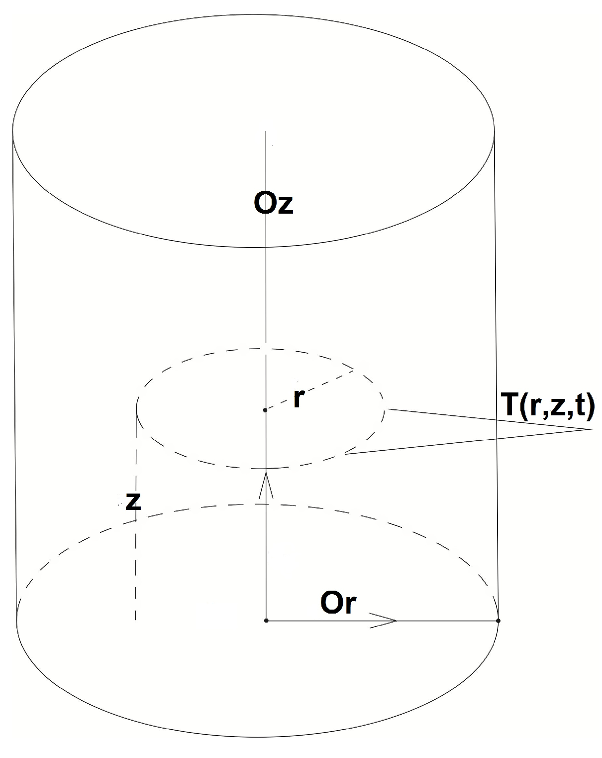
2. Modeling and Mathematical Setting of the Problem
2.1. Main Equation
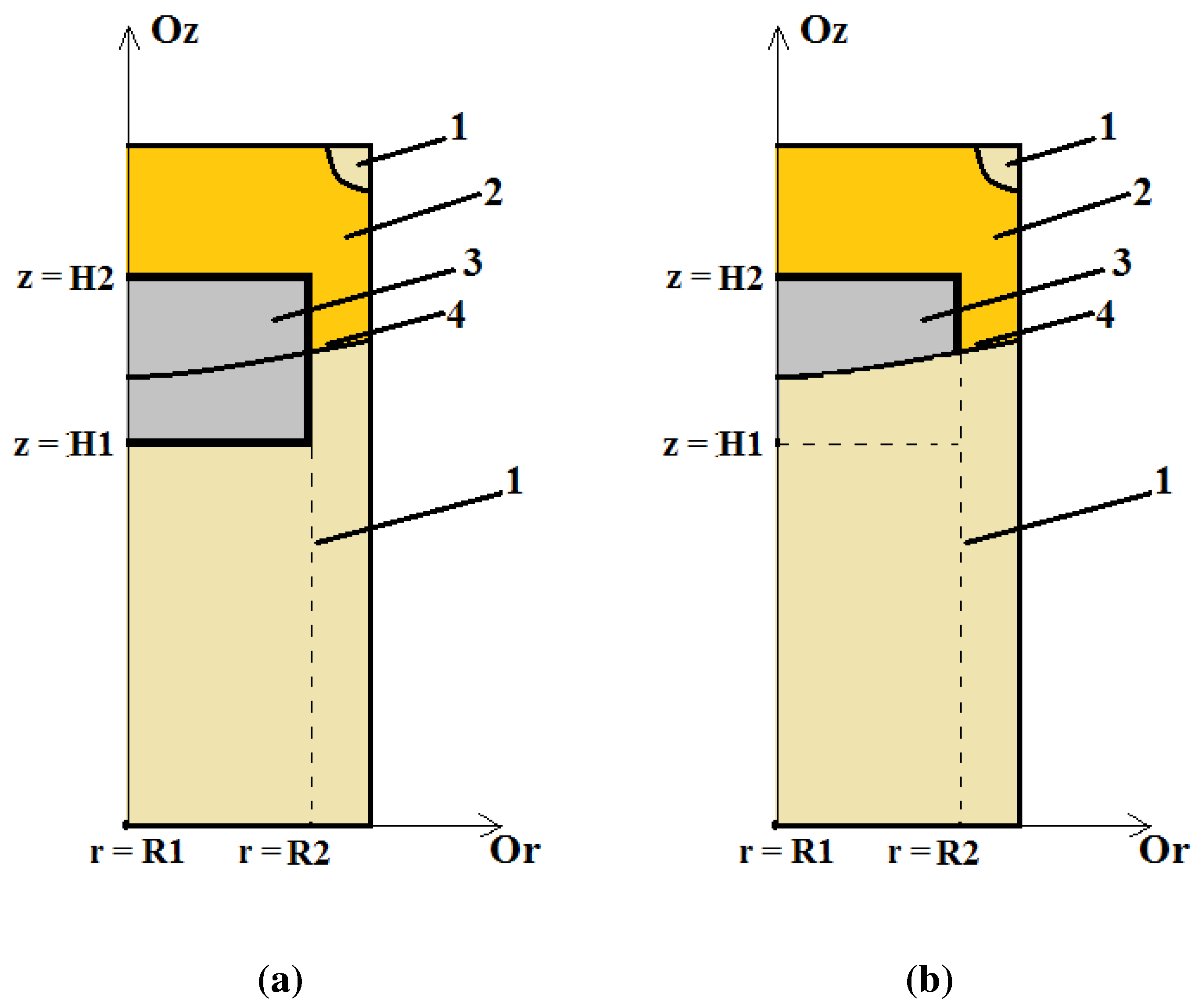
2.2. Equations for the Boundary Conditions
2.3. Heat Streams
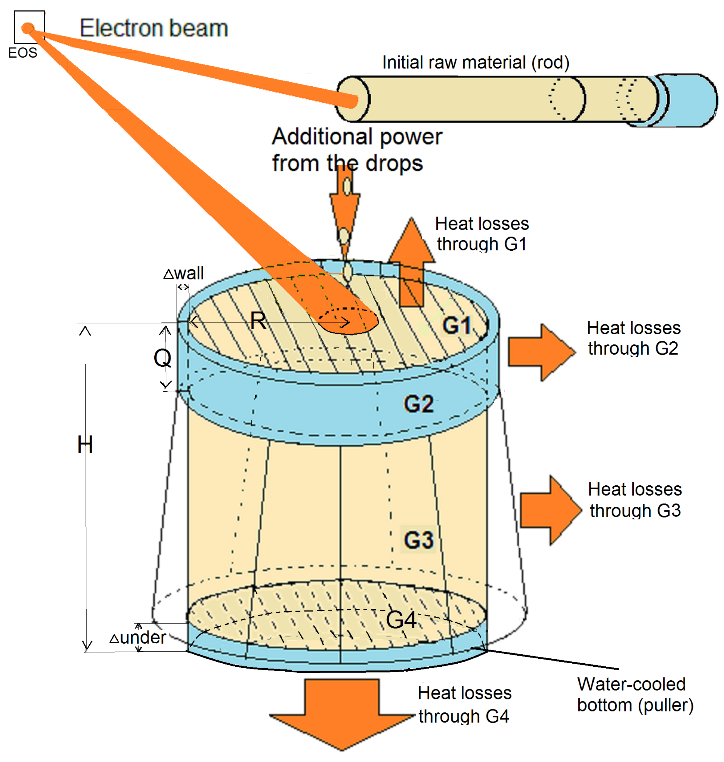
2.3.1. Energy Losses (Radiation and Vapor Losses) through G1:
2.3.2. Streams through the Boundaries G2, G3 and G4:
2.3.3. The Incoming Heat is Determined by the Heating Beam Energy Distribution and by the Heat Added by the Poured Molten Drops :
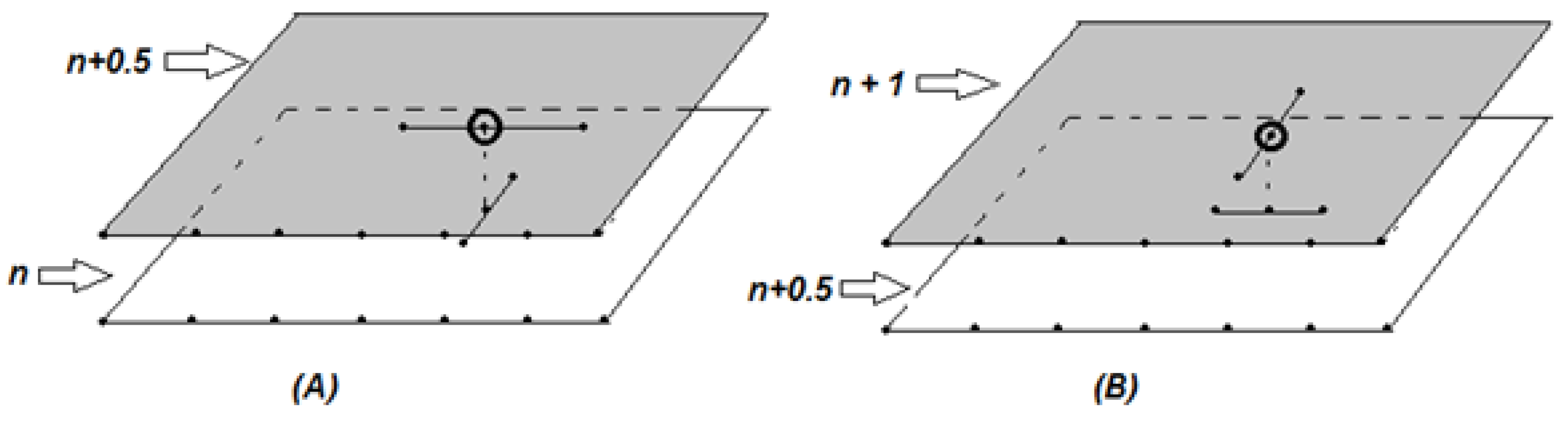
3. Numerical Method
4. Optimization Model and Different Criteria
4.1. Different Criteria
4.2. Discretization of the Criteria
5. Results and Discussion
- Theoretical mathematical modeling of the heating processes during EBMR of metals and alloys, describing the equations of the model;
- Construction of a modified Pismen-Rekford numerical scheme of the model;
- Development of a software for model simulation via the numerical scheme;
- Verification of the model;
- Development of analytical criteria for optimization of the quality of the obtained new materials by achieving flatness of the crystallization front shape;
- Discretization of the criteria synchronically to the numerical discretization of the model and computer implementation;
- Choice of heuristic optimization techniques and synchronization of all developed computer programs;
- Tests using different combinations of criteria, control variables and optimization techniques.

| Parameter | Hf | Cu |
|---|---|---|
| , K | 2506 | 1356 |

| kW | Characteristics | at 10th min | at 15th min | at 20th min | at 30th min | ||||
|---|---|---|---|---|---|---|---|---|---|
| E | S | E | S | E | S | E | S | ||
| 10 | , mm | 50 | 45 | 60 | 60 | 60 | 60 | 60 | 60 |
| , mm | 13 | 12 | 14 | 14 | 17 | 15 | 19 | 15 | |
| 15 | , mm | 60 | 60 | 60 | 60 | 60 | 60 | 60 | 60 |
| , mm | 20 | 20 | 22 | 21 | 19 | 20 | 20 | 20 | |
| No. | , kW | Time of first contact, s |
|---|---|---|
| 1 | 18 | 300 |
| 2 | 20 | 230 |
| 3 | 22 | 180 |
| 4 | 24 | 150 |

6. Conclusions
Acknowledgements
Conflicts of Interest
References
- Mitchell, A.; Wang, T. Electron Beam Melting Technology Review. In Proceedings of the Electron Beam Melting and Refining—State of the Art 2000, Reno, NV, USA, 29–31 October 2000; Bakish, R., Ed.; Bakish Materials Corporation: Englewood, NJ, USA, 2000; pp. 2–13. [Google Scholar]
- Mladenov, G. Electron and Ion Technologies (in Bulgarian); Academic Public House: Sofia, Bulgaria, 2009. [Google Scholar]
- Mladenov, G.; Koleva, E.; Vutova, K.; Vassileva, V. Experimental and theoretical studies of electron beam melting and refining. In Practical Aspects and Applications of Electron Beam Irradiation; Nemtanu, M., Brasoveanu, M., Eds.; Transword Research Network: Trivandrum, India, 2011; pp. 43–93. [Google Scholar]
- Murr, L.; Gaytan, S.; Ramirez, D.; Martinez, E.; Hernandez, J.; Amato, K.; Shindo, P.; Medina, F.; Wicker, R. Metal fabrication by additive manufacturing using laser and electron beam melting technologies. J. Mater. Sci. Technol. 2012, 28, 1–14. [Google Scholar] [CrossRef]
- Bakish, R. Electron Beam Melting 1995 to 2005. In Proceedings of the 7th International EBT Conference, Varna, Bulgaria, 5–10 June 2006; pp. 233–240.
- Choudhury, A.; Hengsberg, E. Electron beam melting and refining of metals and alloys. ISIJ Int. 1992, 32, 673–681. [Google Scholar] [CrossRef]
- Suhas, P. Computational modeling of flow and heat transfer in industrial applications. Int. J. Heat Fluid Flow 2002, 23, 222–231. [Google Scholar]
- Bellot, J.P.; Floris, E.; Jardy, A.; Ablitzer, D. Numerical Simulation of the E.B.C.H.R. Process. In Proceedings of the International Conference Electron Beam Melting and Refining—State of the Art 1993, Reno, NA, USA, 3–5 November 1993; Bakish, R., Ed.; Bakish Materials Corporation: Englewood, NJ, USA, 1993; pp. 139–152. [Google Scholar]
- Westerberg, K.; Clelland, M.; Finlayson, B. Finite element analysis of flow, heat transfer, and free interfaces in an electron-beam vaporization system for metals. Int. J. Numer. Methods Fluid. 1998, 26, 637–655. [Google Scholar] [CrossRef]
- Vutova, K.Zh.; Vassileva, V.I.; Mladenov, G.M. Simulation of the heat transfer process through treated metal, melted in a water-cooled crucible by an electron beam. Vacuum 1997, 48, 143–148. [Google Scholar] [CrossRef]
- Gupta, G.; Marwah, R. Estimation of Effective Thermal Conductivity of Hot Liquid Refractory Metal Generated by Electron Beam Heating. In Proceedings of the International DAE-BRNS Symposium on Electron Beam Technology and Applications, Mumbai, India, 28–30 September 2005; Mascarenhas, M., Kandaswamy, E., Sharma, A., Chakravarthy, D.P., Eds.; Allied Publishers PVT Limited: Mumbai, India, 2005; pp. 371–375. [Google Scholar]
- Vutova, K.Zh.; Koleva, E.G.; Mladenov, G.M. Simulation of thermal transfer process in cast ingots at electron beam melting and refining. Int. Rev. Mech. Eng. 2011, 5, 257–265. [Google Scholar]
- Vutova, K.Zh.; Donchev, V.D.; Vassileva, V.I.; Mladenov, G.M. Thermal transfer process through treated metal regenerated by electron beam melting and refining. J. Metal Sci. Heat Treat 2013, in press. [Google Scholar]
- Ou, J.; Chatterjee, A.; Reilly, C.; Maijer, D.M.; Cockcroft, S.L. Supplemental Proceedings: Materials Processing and Interfaces; John Wiley Sons, Inc.: Hoboken, NJ, USA, 2012; pp. 871–878. [Google Scholar]
- Vutova, K.; Donchev, V.; Vassileva, V.; Mladenov, G. Influence of Process and Thermo-physical Parameters on the Heat Transfer at Electron Beam Melting of Cu and Ta. In Supplemental Proceedings: Materials Processing and Interfaces; John Wiley Sons, Inc.: Hoboken, NJ, USA, 2012; pp. 125–132. [Google Scholar]
- Maijer, D.; Ikeda, T. Mathematical modeling of residual stress formation in electron beam remelting and refining of scrap silicon for the production of solar-grade silicon. Mater. Sci. Eng. A 2011, 390, 188–201. [Google Scholar] [CrossRef]
- Vutova, K.Zh.; Mladenov, G.M. Computer simulation of the heat transfer during electron beam melting and refning. Vacuum 1999, 53, 87–91. [Google Scholar] [CrossRef]
- Koleva, E.; Vutova, K.; Mladenov, G. The role of ingot crucible thermal contact in mathematical modelling of the heat transfer during electron beam melting. Vacuum 2001, 62, 189–196. [Google Scholar] [CrossRef]
- Larikov, L.; Jurchenko, J. Structure and Characteristics of Metals and Alloys. Heat Characteristics of Metals and Alloys (in Russian); Naukova Dumka: Kiev, Russia, 1987. [Google Scholar]
- Samsonov, G. Chemo-Physical Properties of Elements (in Russian); Naukova Dumka: Kiev, Russia, 1965. [Google Scholar]
- Onufriev, S.; Petukhov, V. The thermophysical properties of hafnium in the temperature range from 293 to 2000 K. High Temp. 2008, 46, 203–211. [Google Scholar] [CrossRef]
- Desal, P. Thermodynamic properties of manganese and molybdenum. J. Phys. Chem. Ref. Data 1987, 16, 91–108. [Google Scholar]
- Samarskii, A. Theory of Difference Schemes; Dekker, M., Ed.; CRC Press: New York, NY, USA, 2001. [Google Scholar]
- Vutova, K.; Donchev, V.; Vassileva, V.; Koleva, E.; Mladenov, G. Investigation of Electron Beam Drip Melting by a Time-dependent Heat Model. In Proceedings of the International Conference on High-Power Electron Beam Technology “EBEAM 2012", Reno, NA, USA, 14–16 October 2012; pp. 35–41.
- Donchev, V.; Vutova, K. Optimization method for electron beam melting and refining of metals. J. Phys. Conf. Ser. 2013, in press. [Google Scholar] [CrossRef]
- Vutova, K.; Vassileva, V.; Koleva, E.; Georgieva, E.; Mladenov, G.; Mollov, D.; Kardjiev, M. Investigation of electron beam melting and refining of titanium and tantalum scrap. J. Mater. Process. Technol. 2010, 210, 1089–1094. [Google Scholar] [CrossRef]
© 2013 by the authors; licensee MDPI, Basel, Switzerland. This article is an open access article distributed under the terms and conditions of the Creative Commons Attribution license (http://creativecommons.org/licenses/by/3.0/).
Share and Cite
Vutova, K.; Donchev, V. Electron Beam Melting and Refining of Metals: Computational Modeling and Optimization. Materials 2013, 6, 4626-4640. https://doi.org/10.3390/ma6104626
Vutova K, Donchev V. Electron Beam Melting and Refining of Metals: Computational Modeling and Optimization. Materials. 2013; 6(10):4626-4640. https://doi.org/10.3390/ma6104626
Chicago/Turabian StyleVutova, Katia, and Veliko Donchev. 2013. "Electron Beam Melting and Refining of Metals: Computational Modeling and Optimization" Materials 6, no. 10: 4626-4640. https://doi.org/10.3390/ma6104626