
Estimating the Local Radius of Convergence for Picard Iteration

Department of Informatics, West University of Timisoara, B-dul V. Parvan No. 4, 300223 Timisoara, Romania
Algorithms 2017, 10(1), 10; https://doi.org/10.3390/a10010010
Submission received: 10 October 2016
/
Revised: 28 December 2016
/
Accepted: 30 December 2016
/
Published: 9 January 2017
Abstract
:In this paper, we propose an algorithm to estimate the radius of convergence for the Picard iteration in the setting of a real Hilbert space. Numerical experiments show that the proposed algorithm provides convergence balls close to or even identical to the best ones. As the algorithm does not require to evaluate the norm of derivatives, the computing effort is relatively low.
1. Introduction
The well known Ostrowski theorem [1] gives a sufficient condition (the spectral radius of the Jacobian of the iteration mapping in the fixed point to be less than 1) for the local convergence of Picard iteration. “However, no estimate for the size of an attraction ball is known” [2] (2009). The problem of estimating the local radius of convergence for different iterative methods was considered by numerous authors and several results were obtained particularly for Newton method and its variants. Nevertheless “... effective, computable estimates for convergence radii are rarely available” [3] (1975). A similar remark was made in a more recent paper [4] (2015): “The location of starting approximations, from which the iterative methods converge to a solution of the equation, is a difficult problem to solve”. It is worth noticing that the shape of the attraction basins is an unpredictable and sophisticated set, especially for high order methods, and therefore finding a good ball of convergence for these methods is indeed a difficult task. Among the oldest known results on this topic we could mention those given by Vertgeim, Rall, Rheinboldt, Traub and Wozniakowski, Deuflhard and Potra, Smale [3,5,6,7,8,9]. Relatively recent results were communicated by Argyros [10,11,12], Ferreira [13], Hernandez-Veron and Romero [4], Ren [14], Wang [15].
Deuflhard and Potra [5] proposed the following estimation for Newton method. Let be a nonlinear mapping, where are Banach spaces. Suppose that F is Frchet differentiable on D, that is invertible for each , and that
for all . Under these conditions the equation has a solution . Let such that
and . Then the Newton method remains in and converges to .
In [2] the authors propose a simple and elegant formula to estimate the radius of convergence for Picaed iteration and the algorithm presumptively gives a sharp value. More precisely, let be a nonlinear mapping and a fixed point of G. Suppose that G is differentiable on some ball centred in , , and the derivative of G satisfies
Define
then is an estimation of local convergence radius.
Hernandez and Romero [4] gave the following algorithm for a third-order multi-point method for solving nonlinear equations in Banach spaces [16]. Suppose that p is a solution of the equation, there exists , and is k-Lipschitz continuous on some . Let , where and is the positive real root of a certain algebraic equation of degree three. Then is a local convergence radius. A particular method of this class, which will be investigated in the present study, obtained for a particular value of a numerical parameter of the general class, is the following one point method
In fact this is a modified Newton method in which the derivative is re-evaluated periodically after two steps. Note that, in this particular case, the equation giving the value of , is . We will call (1) the One point Ezquerro-Hernandez method.
Remark 1.
The common way to state that an algorithm (formula) gives the best radius of convergence is to show that for a particular function, there exists a point on the border of the convergence ball for which the conditions of convergence are not satisfied or the considered iteration fails to converge. Several authors who propose an algorithm (formula) and claim that the proposed radius is the best possible, proceed in this way. It would be more satisfactory if the proposed algorithm would be tested for some class of mappings or at least for some test mappings.
Finding a good value for the local convergence radius is rather a difficult task and to find the best one is far more difficult. We propose an algorithm to estimate the radius of convergence for the Picard iteration. Numerical experiments show that the proposed algorithm provides convergence balls close to or even identical to the best ones. It is analogous (but in some details different) with the algorithm for Mann iteration proposed in [17].
From the computational point of view, most algorithms involve the evaluation of Hlder (Lipschitz) constant k of the derivative of the iteration mapping, or of the equation mapping. This evaluation entails solving a constraint optimization problem and the optimum must be global on some ball. Usually, solving this problem is not an easy task, whatever norm of the linear mapping is used. However, using a rough value for k diminishes to some extent the convergence radius estimation. The computational effort of the proposed algorithm, using the vector norm and scalar product, is presumptively lower.
The paper is organized as follows. Some preliminaries are presented in Section 2. Two theorems are proved in Section 3 concerning the local convergence of Picard iteration. The algorithm is described in Section 4. A part of a large number of numerical experiments performed by the author showing that the proposed algorithm gives radii close to the best possible values is presented in Section 5. The computer programs for the main steps of the proposed algorithm are given in Appendix A.
2. Preliminaries
Let be a real Hilbert space with inner product and norm and let C be an open subset of .
We recall the following two basic concepts which are essential for our development: demicontractivity and quasi-expansivity.
A mapping is said to be demicontractive if the set of fixed points of T is nonempty, , and
where . This condition is equivalent to either of the following two:
where . Note that (3) is often more suitable in Hilbert spaces, allowing easier handling of the scalar products and norms. The condition (4) was considered in [18] to prove T-stability of the Picard iteration for this class of mappings. Note that the set of fixed points of a demicontractive mapping is closed and convex [19].
We say that the mapping T is quasi-expansive if
where . If then which justifies the terminology. It is also obvious that the set of fixed points of a mapping T which satisfies (5) consists of a unique element p in C.
3. Local Convergence
The following theorem is the basis of our approach in estimating local radius of convergence. Its proof is similar to the proof of Theorem 1 [22], except in some details. We present the detailed proof here for completeness.
Theorem 1.
Let be a (nonlinear) mapping with nonempty set of fixed points, where C is an open set of a real Hilbert space . Let be a fixed point and let be such that . We shall suppose that (if is bounded and , then this condition is satisfied for any and suitable ). Suppose further that
- (i)
- is demiclosed at zero on C,
- (ii)
- T is demicontractive with on ,then the sequence given by Picard iteration, remains in and converges weakly to some fixed point of T. If, in addition,
- (iii)
- T is quasi-expansive on ,then is the unique fixed point of T in and the sequence converges strongly to .
Proof.
Let p be a fixed point of T. If then, using (ii), we have
Therefore, for any , including , and , i.e., . Moreover, , so that
As is weakly compact and is bounded, there exists a subsequence which converges weakly to q. Then and (i) implies . Suppose now that there exist two subsequences, say and , which converge weakly to u and v respectively. As above, and , . Therefore
Let defined by
We have as . On the other hand, which entails . Therefore .
Finally, from (iii) it results that is the unique fixed point of T in and
so that . ☐
A demicontractive mapping is weak contractive, and a quasi-expansive mapping is weak expansive. The next theorem shows that the demicontractivity and the quasi-expansivity are not contradictory, there exists a relatively large class of mappings which are both demicontractive and quasi-expansive.
Theorem 2.
Let be a (nonlinear) mapping, where C is an open convex subset of . Suppose that , that T is differentiable on C and . Then T is both demicontractive and quasi-expansive on C.
Proof.
(I) T is quasi-expansive on C (therefore consists of a unique element).
Let p be a fixed point of T. Using mean value theorem, for any , we have
Using the notation , we have and . From Banach lemma it results that there exists and . Therefore
that is T is quasi-expansive with .
(II) T is demicontractive on C with .
Due to the condition , we have . Let λ be such that . Consider the quadratic polynomial
The largest zero of P is
and . As and , we have , which entails . For any we have
Taking and , we obtain the condition of demicontracivity. ☐
4. The Algorithm
In finite dimensional spaces the condition of quasi-expansivity is superfluous, since the first two conditions of Theorem 1 are sufficient for the convergence of the Picard iteration. Therefore, in finite dimensional spaces, supposing that the condition (i) of Theorem 1 is fulfilled, we can develop the following algorithm to estimate the local radius of convergence:
Find the largest value for such that
and .
This procedure involves the following main processing:
- Apply a line search algorithm (for example of the type half-step algorithm) on the positive real axis to find the largest value for ;
- At every step of 1 solve the constraint optimization problem (6) and verify the condition .
The main processing of this algorithm is the solution of the constraint optimization problem (6). Therefore we need to use a global constrained optimization method which, generally, has a considerable computational effort. In our experiences we used a population-based metaheuristic method in combination with a local search method.
The algorithm involves an outer iteration (for line search procedure) and an inner iteration (for solving the constrained optimization problem). In N-dimensional spaces, every step of the inner iteration involves evaluations of some functions of N variables each (the components of T), for the computation of and .
Remark 2.
Most of the algorithms for estimation the radius of convergence involve the computation of the optimal Hölder/Lipschitz constant of the derivative of T. This implies evaluations of some functions in N variable each (the components of the derivative of T). Therefore a step of inner iteration involves a polynomial complexity of order 2 combined with the complexity of computing the components of T. The proposed algorithm involves evaluations of components of T, and, presumptively has a lower complexity. However this estimation has only a relative worth, because the main influence on the computational effort is exerted by the global constrained optimization method, which, as it is well known, is a very expensive computation. A good implementation of these algorithms have some positive impact on the computational process.
5. Numerical Experiments
This section is devoted to numerical experiments in order to evaluate the performance of the proposed algorithm. The obtained radii are compared (numerically or graphically) with the maximum radii of convergence. In our experiments the maximum radius was computed by directly checking the convergence of the iteration process starting from all points of a given net of points. The attraction basin (hence the maximum convergence radius) computed in this way has only relative precision. Nevertheless, this method provides significant information about the attraction basins, and the performance of the algorithm from this point of view can be accurately evaluated.
Several numerical experiments in one and several dimensions were performed to validate this method. It is worthwhile to underline that the values obtained by the proposed algorithm are, to some extent, larger than those given by other methods, and, in some cases, our procedure gives local radii of convergence very close to the maximum ones.
5.1. Experiment 1
We have computed the local radius of convergence with the proposed algorithm for One point Ezquerro-Hernandez method and for a number of real functions. In the most these examples the estimated radii are close to (or even coincide with) the maximum radii. For example, in the case of the function and the estimate and the best radius (computed with 15 decimal digits) are identical, .
5.2. Experiment 2
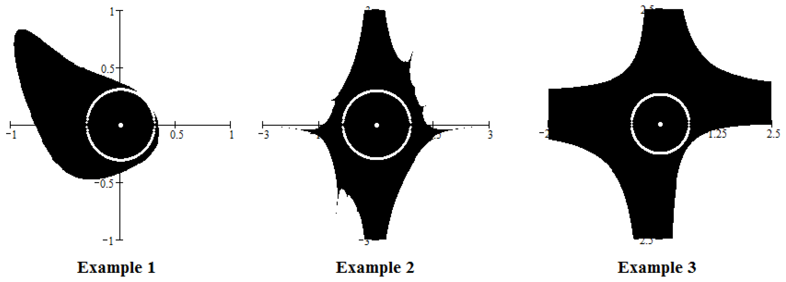
We applied the proposed algorithm to estimate the local radius of convergence for Picard iteration and for a number of mappings in several variables. For the following three test mappings (we will refer to them as Examples 1–3):
the results are given in Figure 1.
The black areas represent the domain of convergence corresponding to the fixed point (for all three examples) and the white circles the local convergence balls. It can be seen that the estimates are satisfactorily close to the best possible ones.
5.3. Experiment 3
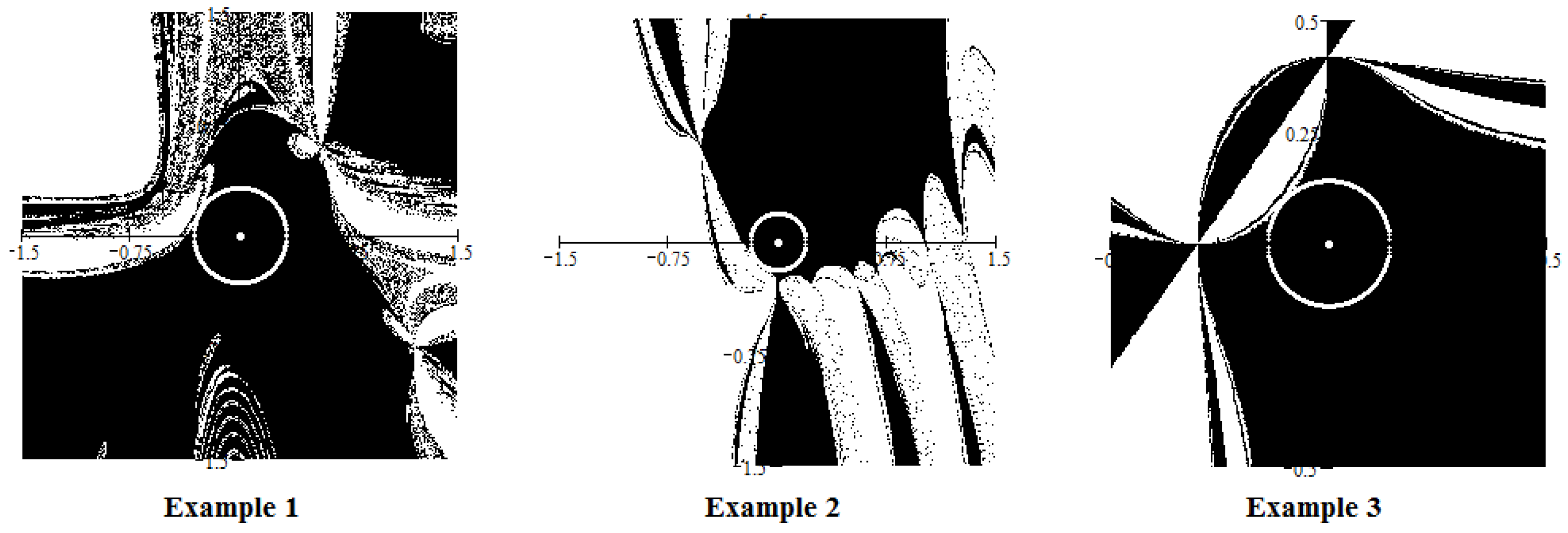
The iteration (1) can be considered as a Picard iteration, , where
Therefore we can apply our algorithm to estimate the local radius of convergence for this method. The results are given in Figure 2.
It can be seen that in this special case the estimates are close (very close) to the best possible radius.
5.4. Experiment 4
In this experiment we estimate numerically the radii of convergence with the proposed algorithm for Picard, Newton and One point Ezquerro-Hernandez methods and for the test mappings. For comparison, we also estimate them by using several other algorithms. In the tables below, we present the results by using the algorithms proposed by Catinas, Deuflhard-Potra and Hernandez-Romero (these algorithms are specifically for considered methods). The last row of each table contains the maximum radii of convergence.
Table 1 contains the results obtained by Catinas and proposed algoritms for the Picard iteration.
The Catinas algorithm requires us to estimate the Hlder (Lipschitz) constant of the derivative of the iteration mapping (7). Even for mappings in two dimensions (which is the case of our test mappings) the computing effort is very high. Therefore, the values for Catinas algorithm in Table 2 are only approximative (we use the sign ≈ to indicate these values). This experiment confirm the results of Experiment 3, the proposed algorithm gives radii very close to the maximim radii for One point Ezquerro-Hernandez method.
Table 3 contains the results obtained by Deuflhard-Potra and proposed algoritms for the Newton method.
The Deuflhard-Potra algorithm gives satisfactory good estimates for Newton method. In the same time this algorithm does not require the evaluation of Hlder (Lipschitz) constant of the derivative of the equation mapping and therefore the computing effort is relatively low. Note that in our experiment the parameter s of the algorithm was chosen , which seems to be most adequate (the algorithm is not very sensitive on this parameter).
Table 2 contains the results obtained by Catinas, Hernandez-Romero and proposed algoritms for the One point Ezquerro-Hernandez method.
6. Conclusions
The proposed algorithm provides radii of convergence close (or very close) to the best possible ones and in some cases (like One point Ezquerro-Hernandez method for one dimension) it seems that the estimates coincide with the maximum radii. As this remarkable characteristic of the proposed algorithm is highlighted in our study only by numerical experiments, it would be a challenge to find the cases in which the two radii are identical.
Conflicts of Interest
The author declares no conflict of interest.
Appendix A
Bellow are given the computer programs for the proposed algorithm, see Figure A1 and Figure A2. To validate the algorithm, numerous numerical experiments were implemented in several ways. To facilitate understanding we present them in MathCad software, which can be easily translated in any other mathematical software systems.
Figure A1.
Computer programs for inner/outer iterations.
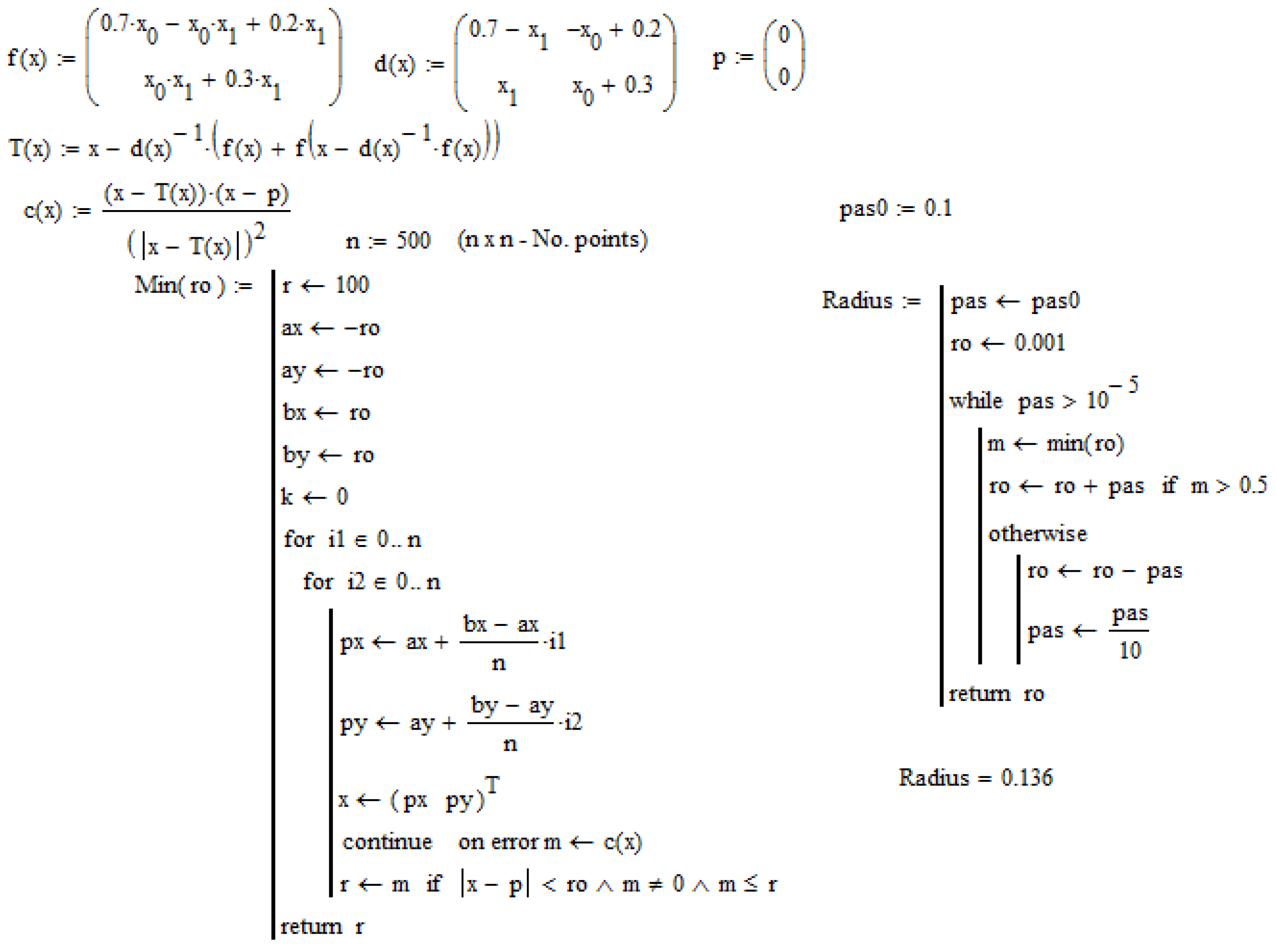
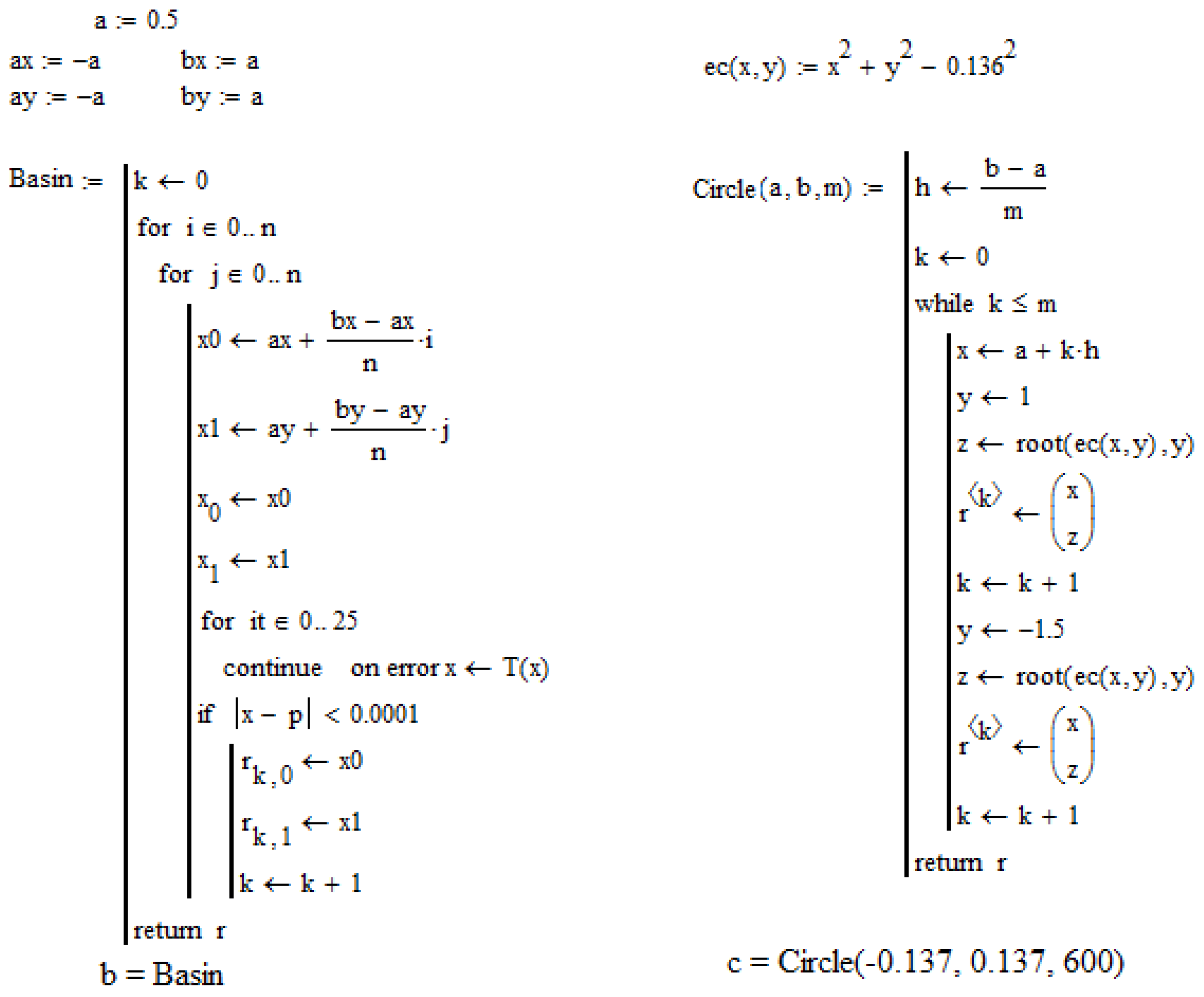
Figure A2.
Computer programs for attraction basin and convergence ball.
Short Computer Programs Description
Min—implements the inner loop of the algorithm. It requires a positive number as input data and provides the global minimum of the cost function (defined in (6) on the ball , corresponding to the iteration function T and to the mapping f. We use here a “brute” method: the cost function is computed on the net of points inside the ball and then the minimum value is chosen. In Figure A1 T is the iteration function for One point Ezquerro-Hernandez method and f is the mapping of Example 3. Note that this program works only for mappings in two variables. For several variables a similar program can be easily developed.
Radius—implements the outer loop of the algorithm. Using a line search technique, it provides the maximum radius of a ball centred in the fixed point, such that the cost function value will be greater than . For the considered example,
Basin—provides a vector containing the points from a given square and belonging to the attraction basin.
Circle—draws a circle centred in the fixed point and with the radius computed by the program Radius.
The mapping F, its derivative, the iteration function T and the cost function c, must be defined outside of the programs. In Figure A1 these elements are defined in the top of the program Min and they are: the mapping F, as in Example 3; the iteration function, as the One point Ezquerro-Hernandez method; the cost function, as proposed in our algorithm. Using a specific graphic function of mathematical software and the vectors b, c, the attraction basin and the estimated ball of convergence can be plotted (Figure 2, Example 3 in our case).
References
- Ostrowski, A.M. Solution of Equations and System of Equations, 2nd ed.; Academic Press: New York, NY, USA, 1966. [Google Scholar]
- Catinas, E. Estimating the radius of an attraction ball. Appl. Math. Lett. 2009, 22, 712–714. [Google Scholar] [CrossRef]
- Rheinboldt, W.C. An adaptive continuation process for solving systems of nonlinear equations. Pol. Acad. Sci. Banach Center Publ. 1975, 3, 129–142. [Google Scholar]
- Hernandez-Veron, M.A.; Romero, N. On the Local Convergence of a Third Order Family of Iterative Processes. Algorithms 2015, 8, 1121–1128. [Google Scholar] [CrossRef]
- Deuflhard, P.; Potra, F.A. Asymptotic mesh independence of Newton-Galerkin Methods via a refined Mysovskii theorem. SIAM J. Numer. Anal. 1992, 29, 1395–1412. [Google Scholar] [CrossRef]
- Rall, L.B. A note on the convergence of Newton method. SIAM J. Numer. Anal. 1974, 11, 34–36. [Google Scholar] [CrossRef]
- Smale, S. Complexity theory and numerical analysis. Acta Numer. 1997, 6, 523–551. [Google Scholar] [CrossRef]
- Traub, J.F.; Wozniakowski, H. Convergence and Complexity of Newton Iteration for Operator Equations. J. Assoc. Comput. Mach. 1979, 26, 250–258. [Google Scholar] [CrossRef]
- Vertgeim, B.A. On conditions for the applicability of Newton’s method. Dokl. Akad. Nauk SSSR 1956, 110, 719–722. [Google Scholar]
- Argyros, I.K. Concerning the radii of convergence for a certain class of Newton-like methods. J. Korea Math. Soc. Educ. Ser. B: Pure Appl. Math. 2008, 15, 47–55. [Google Scholar]
- Argyros, I.K. Concerning the “terra ingognita” between convergence regions of two Newton methods. Nonlinear Anal. 2005, 62, 179–194. [Google Scholar] [CrossRef]
- Argyros, I.K. A unifyng local-semilocal convergence analysis and applications for two-points Newton methods in Banach spaces. J. Math. Anal. Appl. 2004, 298, 374–397. [Google Scholar] [CrossRef]
- Frerreira, O.P. Local convergence of Newton method in Banach spaces from the viewpoint of the majorant principle. IMA J. Numer. Anal. 2009, 29, 746–759. [Google Scholar] [CrossRef]
- Ren, H. On the local convergence of a deformed Newton method under Argyros-type conditions. J. Math. Anal. Appl. 2006, 321, 396–404. [Google Scholar] [CrossRef]
- Wang, X. Convergence of Newton’s method and uniquenees of the solution of equations in Banach space. IMA J. Numer. Anal. 2000, 20, 123–134. [Google Scholar] [CrossRef]
- Ezquerro, J.A.; Hernandez, M.A. An optimization of Chebyshev’s method. J. Complex. 2009, 25, 343–361. [Google Scholar] [CrossRef]
- Maruster, S. Local convergence radius for the Mann-type iteration. Anal. Univ. Vest Timisoara Seria Mat. Inf. LIII 2015, 53, 109–120. [Google Scholar]
- Qing, Y.; Rhoades, B.E. T-stability of Picard iteration in metric spaces. Fixed Point Theory Appl. Hindawi Publ. Corp. 2008, 2008. [Google Scholar] [CrossRef]
- Marino, G.; Xu, H.-K. Weak and strong convergence theorems for strict pseudo-contractions in Hilbert spaces. J. Math. Anal. Appl. 2007, 329, 336–346. [Google Scholar] [CrossRef]
- Outlaw, C.L. Mean value iteration for nonexpansive mappings in a Banach space. Pac. J. Math. 1969, 30, 747–759. [Google Scholar] [CrossRef]
- Senter, H.F.; Dotson, W.G., Jr. Approximating fixed points of nonexpansive mappings. Proc. Am. Math. Soc. 1974, 44, 375–380. [Google Scholar] [CrossRef]
- Maruster, S. The solution by iteration of nonlinear equations in Hilbert spaces. Proc. Am. Math. Soc. 1977, 63, 69–73. [Google Scholar] [CrossRef]
Figure 1.
The estimates with the proposed algorithm for Picard iteration.

Figure 2.
The estimates with the proposed algorithm for One point Ezquerro-Hernandez method.


| Method | Example 1 | Example 2 | Example 3 |
|---|---|---|---|
| Catinas algorithm | 0.200000 | 0.430017 | 0.376876 |
| Proposed algorithm | 0.307939 | 0.896639 | 0.645209 |
| Maximum radius | 0.311608 | 1.240665 | 0.806039 |
| Method | Example 1 | Example 2 | Example 3 |
|---|---|---|---|
| Catinas algorithm | ≈0.194442 | ≈0.114921 | ≈0.081090 |
| Hernandez-Romero algorithm | 0.221114 | 0.146160 | 0.111906 |
| Proposed algorithm | 0.319185 | 0.191426 | 0.136057 |
| Maximum radius | 0.319217 | 0.197430 | 0.137130 |
| Method | Example 1 | Example 2 | Example 3 |
|---|---|---|---|
| Deuflhard-Potra algorithm | 0.346083 | 0.200051 | 0.162746 |
| Proposed algorithm | 0.363135 | 0.236905 | 0.163737 |
| Maximum radius | 0.446068 | 0.254446 | 0.244121 |
© 2017 by the author. Licensee MDPI, Basel, Switzerland. This article is an open access article distributed under the terms and conditions of the Creative Commons Attribution (CC BY) license ( http://creativecommons.org/licenses/by/4.0/).
Share and Cite
MDPI and ACS Style
Măruşter, Ş. Estimating the Local Radius of Convergence for Picard Iteration. Algorithms 2017, 10, 10. https://doi.org/10.3390/a10010010
AMA Style
Măruşter Ş. Estimating the Local Radius of Convergence for Picard Iteration. Algorithms. 2017; 10(1):10. https://doi.org/10.3390/a10010010
Chicago/Turabian StyleMăruşter, Ştefan. 2017. "Estimating the Local Radius of Convergence for Picard Iteration" Algorithms 10, no. 1: 10. https://doi.org/10.3390/a10010010
Note that from the first issue of 2016, this journal uses article numbers instead of page numbers. See further details here.