
Coupled Least Squares Identification Algorithms for Multivariate Output-Error Systems

Abstract
:1. Introduction
- for multivariate output-error systems, this paper derives two coupled least squares parameter estimation algorithms by using the auxiliary model identification idea and the coupling identification concept;
- the proposed algorithms can generate more accurate parameter estimates, and avoid computing the matrix inversion in the multivariable RLS algorithm, for the purpose of reducing computational load.
2. System Description and Identification Model
3. The Multivariate Auxiliary Model Coupled Identification Algorithm
3.1. The Auxiliary Model Based Recursive Least Squares Algorithm
- Set the initial values: , , , , , 2, ⋯, , . Set the data length L.
- Collect the observation data {, } and form the information matrix by (10).
- Update the parameter estimation vector by (6).
- Compute the output of the auxiliary model using (11).
- If , stop the recursive computation and obtain the parameter estimates; otherwise, increase t by 1 and go to Step 2.
3.2. The Coupled Subsystem Auxiliary Model Based Recursive Least Squares Algorithm
- Set the initial values: , , , , , 2, ⋯, , . Set the data length L.
- Collect the observation data {, } and form the information matrix by (22).
- If , stop the recursive computation and obtain the parameter estimates; otherwise, increase t by 1 and go to Step 2.
3.3. The Coupled Auxiliary Model Based Recursive Least Squares Algorithm
- Set the initial values: , , , , , 2, ⋯, , . Set the data length L.
- Obtain the parameter estimation vector and compute by (35).
- If , stop the recursive computation and obtain the parameter estimates; otherwise, increase t by 1 and go to Step 2.
4. Examples
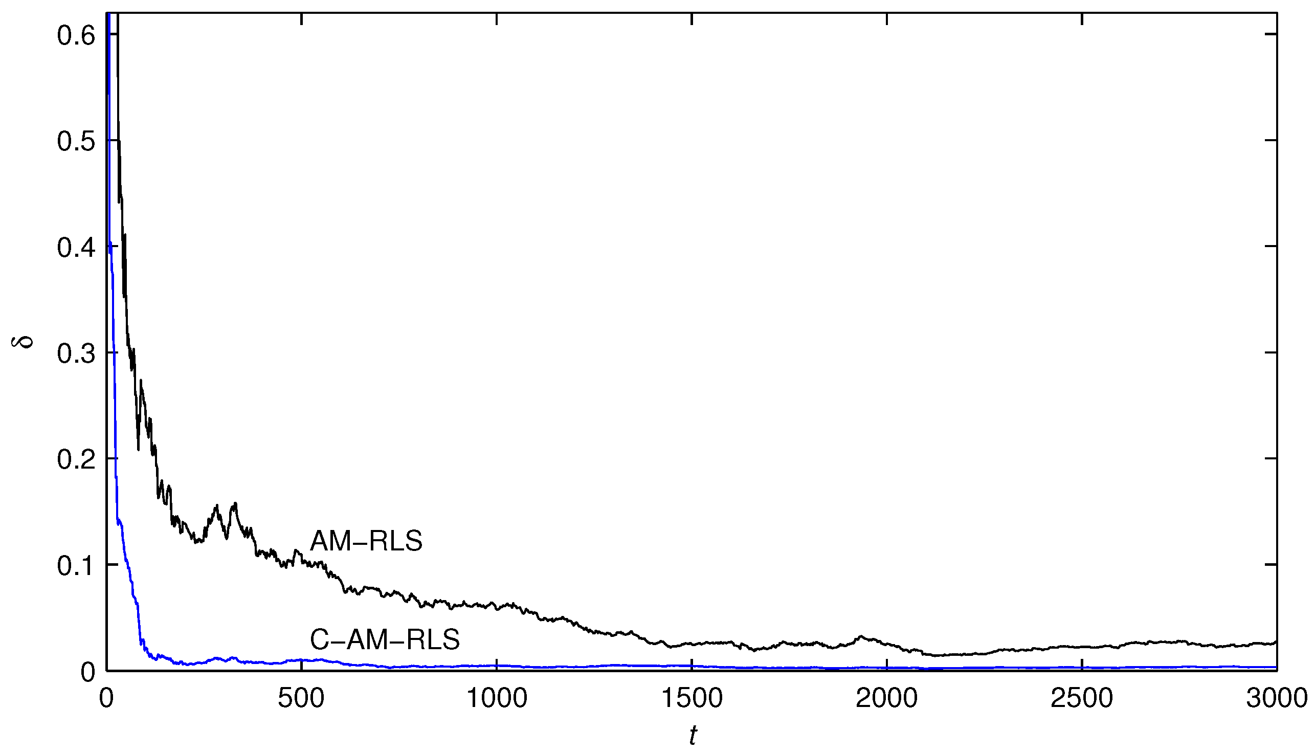
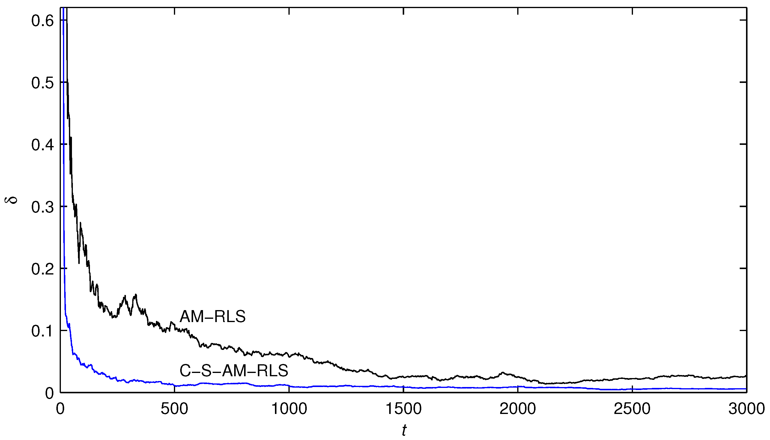
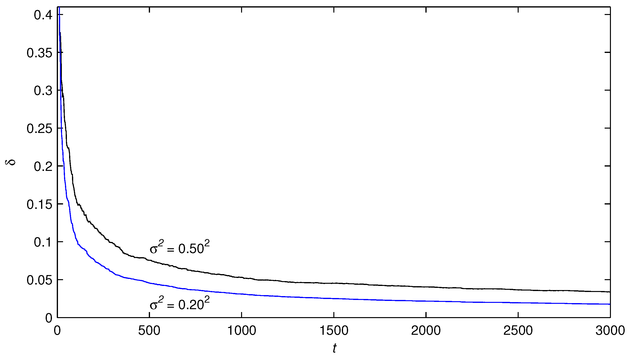
- The parameter estimation errors by the presented algorithms become smaller and smaller and go to zero with the increasing of time t.
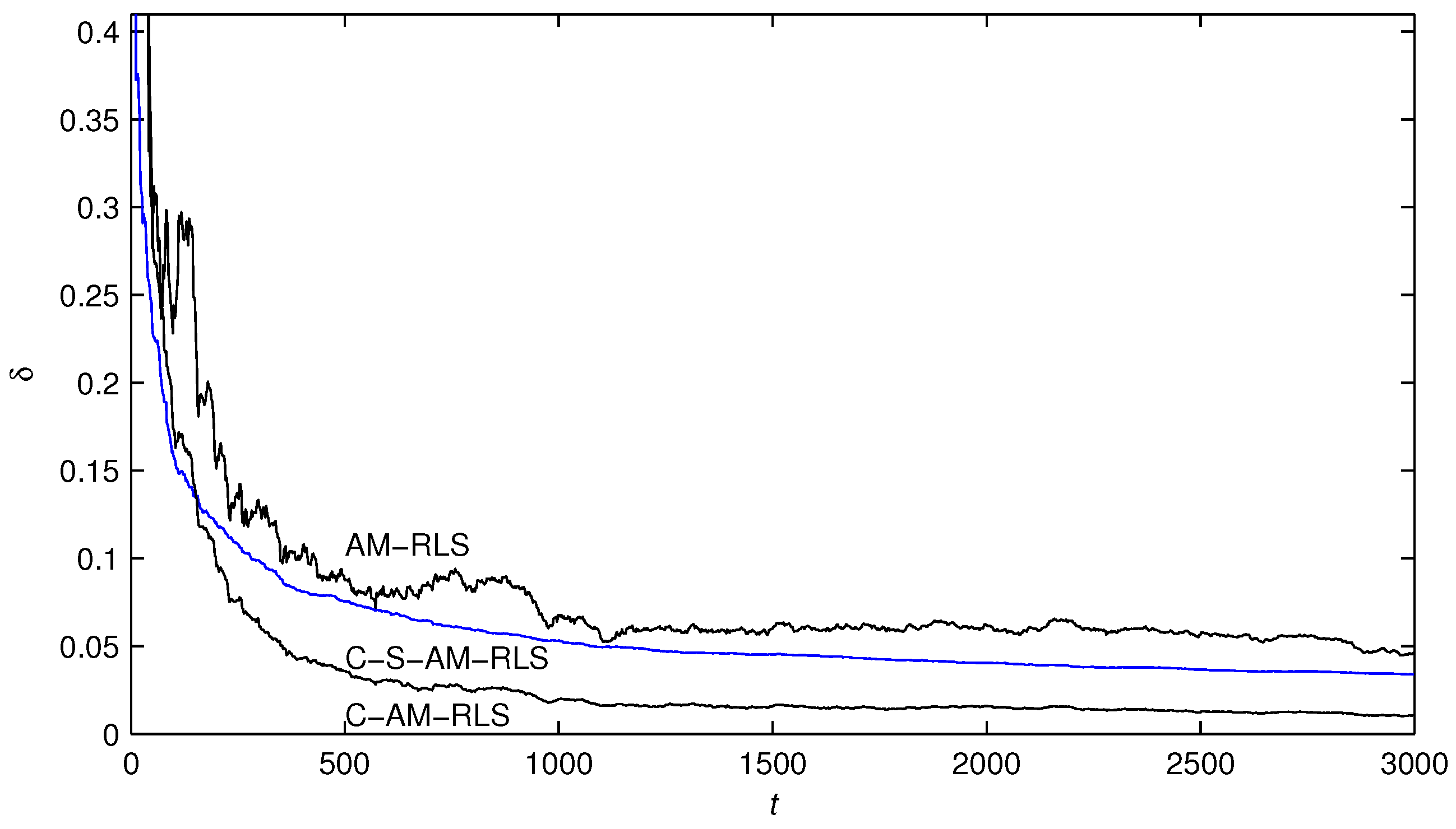
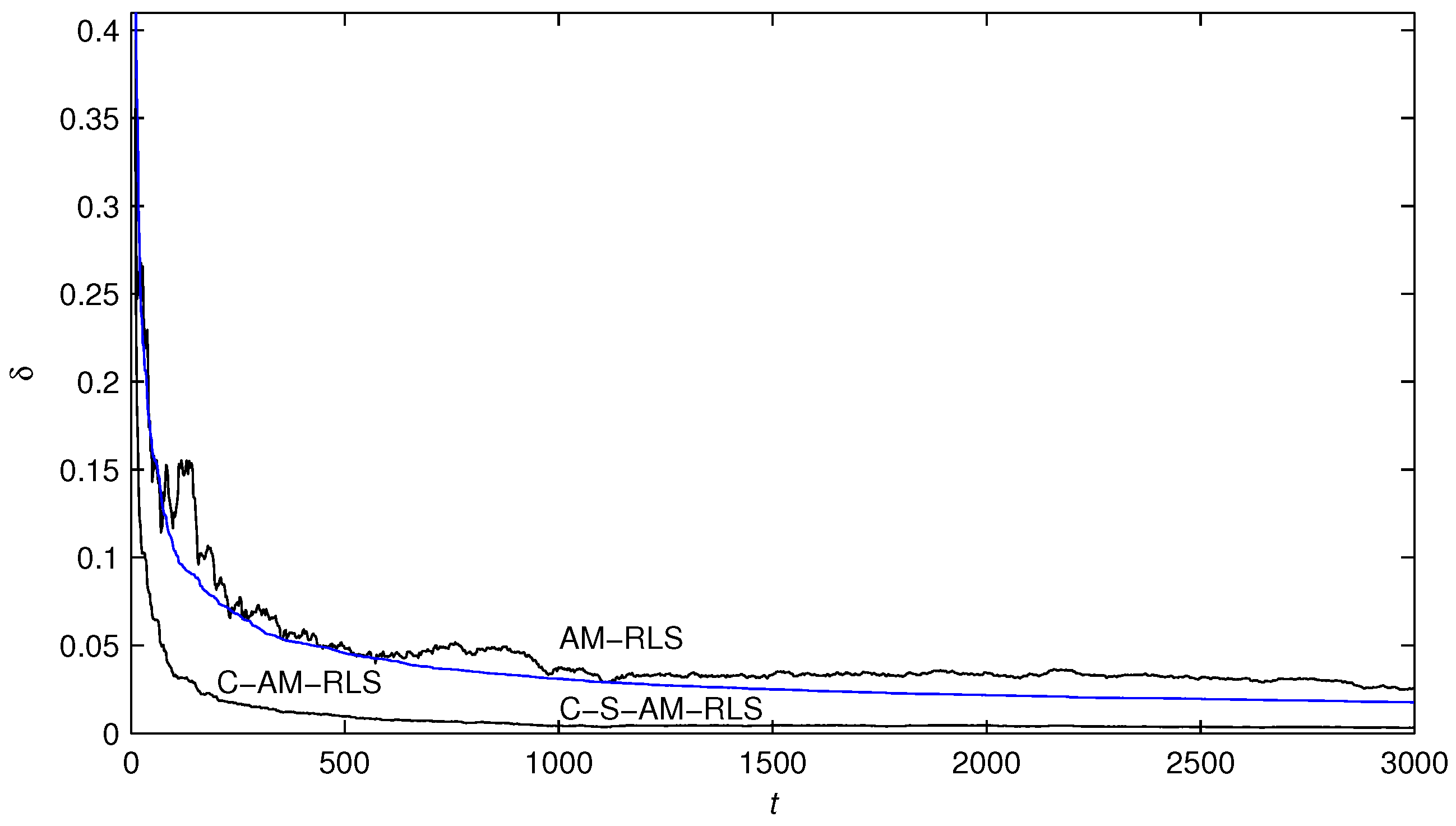
- In contrast to the AM-RLS algorithm, the proposed C-S-AM-RLS and C-AM-RLS algorithms have faster convergence rates and more accurate parameter estimates with the same simulation conditions.
- In contrast to the AM-RLS algorithm, the proposed C-S-AM-RLS and C-AM-RLS algorithms have faster convergence rates and more accurate parameter estimates with the same simulation conditions, and the C-AM-RLS algorithm can obtain the most accurate estimates for the system parameters.
5. Conclusions
- The C-S-AM-RLS algorithm and the C-AM-RLS algorithm are presented by forming a coupled relationship between the parameter estimation vectors of the subsystems, and they avoid computing the matrix inversion in the multivariable AM-RLS algorithm so they require lower computational load and achieve highly accurate parameter estimates.
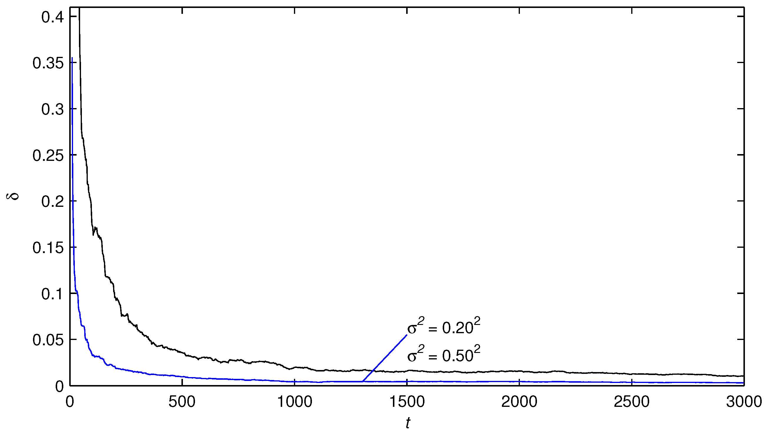
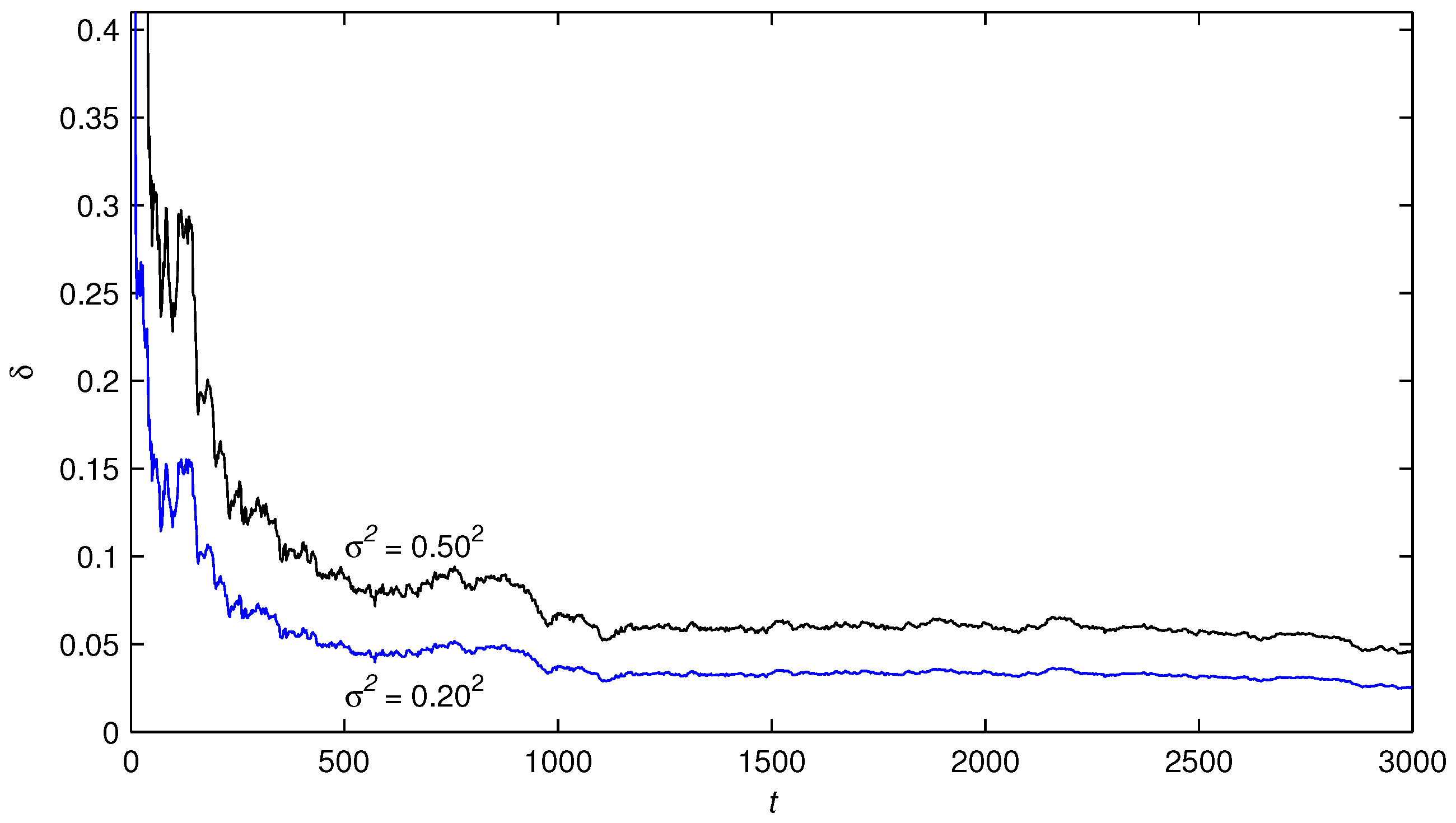
- With the noise-to-signal ratios decreasing, the parameter estimation errors given by the proposed algorithms become smaller.
Acknowledgments
Author Contributions
Conflicts of Interest
References
- Ding, F. System Identification—New Theory and Methods; Science Press: Beijing, China, 2013. [Google Scholar]
- Ding, F. System Identification—Performances Analysis for Identification Methods; Science Press: Beijing, China, 2014. [Google Scholar]
- Ding, F. System Identification—Multi-Innovation Identification Theory and Methods; Science Press: Beijing, China, 2016. [Google Scholar]
- Liu, Y.J.; Tao, T.Y. A CS recovery algorithm for model and time delay identification of MISO-FIR systems. Algorithms 2015, 8, 743–753. [Google Scholar] [CrossRef]
- Ding, J.L. Data filtering based recursive and iterative least squares algorithms for parameter estimation of multi-input output systems. Algorithms 2016, 9. [Google Scholar] [CrossRef]
- Tsubakino, D.; Krstic, M.; Oliveira, T.R. Exact predictor feedbacks for multi-input LTI systems with distinct input delays. Automatica 2016, 71, 143–150. [Google Scholar] [CrossRef]
- Tian, Y.; Jin, Q.W.; Lavery, J.E. ℓ1 Major component detection and analysis (ℓ1 MCDA): Foundations in two dimensions. Algorithms 2013, 6, 12–28. [Google Scholar] [CrossRef]
- Zhang, X.Y.; Hoagg, J.B. Subsystem identification of multivariable feedback and feedforward systems. Automatica 2016, 72, 131–137. [Google Scholar] [CrossRef]
- Salhi, H.; Kamoun, S. A recursive parametric estimation algorithm of multivariable nonlinear systems described by Hammerstein mathematical models. Appl. Math. Model. 2015, 39, 4951–4962. [Google Scholar] [CrossRef]
- Wang, Y.J.; Ding, F. Novel data filtering based parameter identification for multiple-input multiple-output systems using the auxiliary model. Automatica 2016, 71, 308–313. [Google Scholar] [CrossRef]
- Zhang, Y.; Zhao, Z.; Cui, G.M. Auxiliary model method for transfer function estimation from noisy input and output data. Appl. Math. Model. 2015, 39, 4257–4265. [Google Scholar] [CrossRef]
- Li, P.; Feng, J.; de Lamare, R.C. Robust rank reduction algorithm with iterative parameter optimization and vector perturbation. Algorithms 2015, 8, 573–589. [Google Scholar] [CrossRef]
- Filipovic, V.Z. Consistency of the robust recursive Hammerstein model identification algorithm. J. Frankl. Inst. 2015, 352, 1932–1945. [Google Scholar] [CrossRef]
- Guo, L.J.; Wang, Y.J.; Wang, C. A recursive least squares algorithm for pseudo-linear arma systems using the auxiliary model and the filtering technique. Circuits Syst. Signal Process. 2016, 35, 2655–2667. [Google Scholar] [CrossRef]
- Meng, D.D.; Ding, F. Model equivalence-based identification algorithm for equation-error systems with colored noise. Algorithms 2015, 8, 280–291. [Google Scholar] [CrossRef]
- Wang, D.Q.; Zhang, W. Improved least squares identification algorithm for multivariable Hammerstein systems. J. Frankl. Inst. 2015, 352, 5292–5307. [Google Scholar] [CrossRef]
- Wu, C.Y.; Tsai, J.S.H.; Guo, S.M. A novel on-line observer/Kalman filter identification method and its application to input-constrained active fault-tolerant tracker design for unknown stochastic systems. J. Frankl. Inst. 2015, 352, 1119–1151. [Google Scholar] [CrossRef]
- Bako, L. Adaptive identification of linear systems subject to gross errors. Automatica 2016, 67, 192–199. [Google Scholar] [CrossRef]
- Ding, F.; Liu, G.; Liu, X.P. Parameter estimation with scarce measurements. Automatica 2011, 47, 1646–1655. [Google Scholar] [CrossRef]
- Jin, Q.B.; Wang, Z.; Liu, X.P. Auxiliary model-based interval-varying multi-innovation least squares identification for multivariable OE-like systems with scarce measurements. J. Process Control 2015, 35, 154–168. [Google Scholar] [CrossRef]
- Wang, C.; Tang, T. Recursive least squares estimation algorithm applied to a class of linear-in-parameters output-error moving average systems. Appl. Math. Lett. 2014, 29, 36–41. [Google Scholar] [CrossRef]
- Ding, F. Coupled-least-squares identification for multivariable systems. IET Control Theory Appl. 2013, 7, 68–79. [Google Scholar] [CrossRef]
- Radenkovic, M.; Tadi, M. Self-tuning average consensus in complex networks. J. Frankl. Inst. 2015, 352, 1152–1168. [Google Scholar] [CrossRef]
- Ding, F.; Liu, G.; Liu, X.P. Partially coupled stochastic gradient identification methods for non-uniformly sampled systems. IEEE Trans. Autom. Control 2010, 55, 1976–1981. [Google Scholar] [CrossRef]
- Eldem, V.; Şahan, G. The effect of coupling conditions on the stability of bimodal systems in R3. Syst. Control Lett. 2016, 96, 141–150. [Google Scholar] [CrossRef]
- Wu, K.N.; Tian, T.; Wang, L.M. Synchronization for a class of coupled linear partial differential systems via boundary control. J. Frankl. Inst. 2016, 353, 4062–4073. [Google Scholar] [CrossRef]
- Meng, D.D. Recursive least squares and multi-innovation gradient estimation algorithms for bilinear stochastic systems. Circuits Syst. Signal Process. 2016, 35. [Google Scholar] [CrossRef]
- Wang, Y.J.; Ding, F. The filtering based iterative identification for multivariable systems. IET Control Theory Appl. 2016, 10, 894–902. [Google Scholar] [CrossRef]
- Wang, T.Z.; Qi, J.; Xu, H. Fault diagnosis method based on FFT-RPCA-SVM for cascaded-multilevel inverter. ISA Trans. 2016, 60, 156–163. [Google Scholar] [CrossRef] [PubMed]
- Wang, T.Z.; Wu, H.; Ni, M.Q. An adaptive confidence limit for periodic non-steady conditions fault detection. Mech. Syst. Signal Process. 2016, 72–73, 328–345. [Google Scholar] [CrossRef]
- Feng, L.; Wu, M.H.; Li, Q.X. Array factor forming for image reconstruction of one-dimensional nonuniform aperture synthesis radiometers. IEEE Geosci. Remote Sens. Lett. 2016, 13, 237–241. [Google Scholar] [CrossRef]


| t | |||||||
|---|---|---|---|---|---|---|---|
| 100 | 0.19169 | 0.46405 | −0.29921 | 0.51505 | −0.69003 | 0.56147 | 24.77137 |
| 200 | 0.24129 | 0.55426 | −0.26362 | 0.52514 | −0.61030 | 0.56009 | 13.91359 |
| 500 | 0.24361 | 0.55706 | −0.24361 | 0.47651 | −0.56945 | 0.53294 | 10.96959 |
| 1000 | 0.29857 | 0.61286 | −0.24654 | 0.45360 | −0.55928 | 0.57197 | 5.78088 |
| 2000 | 0.31147 | 0.64219 | −0.23371 | 0.47639 | −0.51822 | 0.57977 | 2.53112 |
| 3000 | 0.31743 | 0.65208 | −0.23405 | 0.47050 | −0.48951 | 0.55819 | 2.65000 |
| True values | 0.30000 | 0.64000 | −0.25000 | 0.47000 | −0.50000 | 0.57000 |
| t | |||||||
|---|---|---|---|---|---|---|---|
| 100 | 0.29097 | 0.63357 | −0.27254 | 0.45781 | −0.49700 | 0.52648 | 4.44497 |
| 200 | 0.29760 | 0.62737 | −0.26354 | 0.45916 | −0.50241 | 0.54735 | 2.69357 |
| 500 | 0.29689 | 0.63747 | −0.25217 | 0.46685 | −0.50539 | 0.55960 | 1.11229 |
| 1000 | 0.29887 | 0.63910 | −0.25196 | 0.46698 | −0.50283 | 0.55826 | 1.08848 |
| 2000 | 0.30151 | 0.63810 | −0.24935 | 0.46850 | −0.50098 | 0.55961 | 0.92996 |
| 3000 | 0.30313 | 0.63900 | −0.24647 | 0.46872 | −0.50302 | 0.56643 | 0.58689 |
| True values | 0.30000 | 0.64000 | −0.25000 | 0.47000 | −0.50000 | 0.57000 |
| t | |||||||
|---|---|---|---|---|---|---|---|
| 100 | 0.29005 | 0.63637 | −0.25615 | 0.45607 | −0.49231 | 0.58483 | 2.14162 |
| 200 | 0.29623 | 0.64525 | −0.25140 | 0.46821 | −0.50367 | 0.57151 | 0.67931 |
| 500 | 0.29686 | 0.63477 | −0.25512 | 0.47214 | −0.50108 | 0.56153 | 1.01842 |
| 1000 | 0.30266 | 0.64036 | −0.24782 | 0.46668 | −0.50268 | 0.57115 | 0.48179 |
| 2000 | 0.30091 | 0.64021 | −0.24740 | 0.46931 | −0.50116 | 0.57056 | 0.26815 |
| 3000 | 0.30202 | 0.64160 | −0.24831 | 0.46919 | −0.49823 | 0.56821 | 0.34814 |
| True values | 0.30000 | 0.64000 | −0.25000 | 0.47000 | −0.50000 | 0.57000 |
| σ | t | |||||||||||
|---|---|---|---|---|---|---|---|---|---|---|---|---|
| 0.50 | 100 | −0.07767 | −0.05531 | −0.36662 | 0.24956 | 0.48032 | −0.31206 | 0.31519 | −0.06257 | 0.41747 | 0.62394 | 24.42046 |
| 200 | −0.12975 | −0.19484 | −0.39270 | 0.19552 | 0.54739 | −0.39801 | 0.25127 | −0.15292 | 0.40869 | 0.59869 | 15.11250 | |
| 500 | −0.19310 | −0.17229 | −0.36609 | 0.20923 | 0.61180 | −0.37565 | 0.30089 | −0.22450 | 0.47133 | 0.60444 | 8.75946 | |
| 1000 | −0.19356 | −0.18464 | −0.35077 | 0.26929 | 0.61180 | −0.40097 | 0.29274 | −0.24058 | 0.41768 | 0.58457 | 6.77306 | |
| 2000 | −0.16577 | −0.16642 | −0.35510 | 0.26588 | 0.63592 | −0.38138 | 0.27095 | −0.24643 | 0.43211 | 0.58239 | 6.17573 | |
| 3000 | −0.17437 | −0.15862 | −0.34955 | 0.26143 | 0.63990 | −0.38157 | 0.26516 | −0.24155 | 0.41820 | 0.59485 | 4.64800 | |
| 0.20 | 100 | −0.14504 | −0.09948 | −0.34108 | 0.24926 | 0.56565 | −0.34426 | 0.29779 | −0.13584 | 0.40947 | 0.62501 | 12.55557 |
| 200 | −0.16080 | −0.17384 | −0.35653 | 0.21984 | 0.59626 | −0.38955 | 0.26341 | −0.18663 | 0.40729 | 0.60783 | 8.16496 | |
| 500 | −0.19361 | −0.16177 | −0.34130 | 0.22732 | 0.62940 | −0.37772 | 0.29134 | −0.22686 | 0.44372 | 0.61191 | 4.82443 | |
| 1000 | −0.19260 | −0.16915 | −0.33276 | 0.26075 | 0.62898 | −0.39165 | 0.28698 | −0.23581 | 0.41417 | 0.60050 | 3.75051 | |
| 2000 | −0.17637 | −0.15883 | −0.33513 | 0.25880 | 0.64247 | −0.38068 | 0.27492 | −0.23911 | 0.42227 | 0.59904 | 3.43136 | |
| 3000 | −0.18131 | −0.15460 | −0.33203 | 0.25635 | 0.64460 | −0.38087 | 0.27172 | −0.23640 | 0.41457 | 0.60604 | 2.58030 | |
| True values | −0.19000 | −0.15000 | −0.31000 | 0.25000 | 0.65000 | −0.38000 | 0.28000 | −0.23000 | 0.41000 | 0.62000 | ||
| σ | t | |||||||||||
|---|---|---|---|---|---|---|---|---|---|---|---|---|
| 0.50 | 100 | −0.21759 | −0.11924 | −0.38525 | 0.15721 | 0.63656 | −0.34223 | 0.29058 | −0.20577 | 0.37492 | 0.48917 | 15.79715 |
| 200 | −0.20637 | −0.14535 | −0.37445 | 0.17481 | 0.63617 | −0.35041 | 0.28941 | −0.21028 | 0.38068 | 0.52643 | 12.03360 | |
| 500 | −0.20820 | −0.15449 | −0.35370 | 0.20271 | 0.64497 | −0.35998 | 0.29075 | −0.22235 | 0.40008 | 0.56361 | 7.55407 | |
| 1000 | −0.20219 | −0.15807 | −0.34231 | 0.22279 | 0.64575 | −0.36723 | 0.28829 | −0.22609 | 0.39938 | 0.57785 | 5.31882 | |
| 2000 | −0.19351 | −0.15523 | −0.33660 | 0.23115 | 0.65084 | −0.36868 | 0.28424 | −0.22807 | 0.40408 | 0.58666 | 4.04352 | |
| 3000 | −0.19451 | −0.15372 | −0.33290 | 0.23487 | 0.65196 | −0.37059 | 0.28273 | −0.22881 | 0.40384 | 0.59231 | 3.39624 | |
| 0.20 | 100 | −0.22599 | −0.13897 | −0.32193 | 0.22250 | 0.58332 | −0.31192 | 0.25836 | −0.21204 | 0.39836 | 0.55805 | 10.49246 |
| 200 | −0.22086 | −0.15125 | −0.32183 | 0.22627 | 0.60226 | −0.33263 | 0.26598 | −0.21525 | 0.40181 | 0.57614 | 7.64726 | |
| 500 | −0.21073 | −0.15254 | −0.31739 | 0.23480 | 0.62239 | −0.35282 | 0.27247 | −0.22272 | 0.40840 | 0.59331 | 4.55688 | |
| 1000 | −0.20374 | −0.15441 | −0.31579 | 0.24128 | 0.63135 | −0.36182 | 0.27507 | −0.22497 | 0.40834 | 0.60063 | 3.11396 | |
| 2000 | −0.19848 | −0.15281 | −0.31510 | 0.24388 | 0.63828 | −0.36705 | 0.27614 | −0.22659 | 0.40919 | 0.60523 | 2.17345 | |
| 3000 | −0.19699 | −0.15245 | −0.31444 | 0.24521 | 0.64095 | −0.36950 | 0.27665 | −0.22739 | 0.40911 | 0.60772 | 1.76930 | |
| True values | −0.19000 | −0.15000 | −0.31000 | 0.25000 | 0.65000 | −0.38000 | 0.28000 | −0.23000 | 0.41000 | 0.62000 | ||
| σ | t | |||||||||||
|---|---|---|---|---|---|---|---|---|---|---|---|---|
| 0.50 | 100 | −0.14313 | −0.08944 | −0.29923 | 0.14967 | 0.60004 | −0.48000 | 0.27048 | −0.10880 | 0.39393 | 0.64199 | 17.32565 |
| 200 | −0.15590 | −0.16031 | −0.30620 | 0.18954 | 0.60690 | −0.43088 | 0.26046 | −0.17047 | 0.40328 | 0.61953 | 9.53865 | |
| 500 | −0.18908 | −0.15426 | −0.31365 | 0.22262 | 0.63038 | −0.39293 | 0.27930 | −0.21346 | 0.42501 | 0.61348 | 3.57545 | |
| 1000 | −0.18864 | −0.15914 | −0.31439 | 0.24558 | 0.63487 | −0.38941 | 0.28005 | −0.22501 | 0.41240 | 0.60972 | 1.98417 | |
| 2000 | −0.18100 | −0.15438 | −0.31763 | 0.24933 | 0.64474 | −0.38309 | 0.27657 | −0.23004 | 0.41637 | 0.60902 | 1.58563 | |
| 3000 | −0.18721 | −0.15257 | −0.31714 | 0.24959 | 0.64668 | −0.38257 | 0.27582 | −0.23014 | 0.41296 | 0.61247 | 1.06366 | |
| 0.20 | 100 | −0.18575 | −0.14611 | −0.32571 | 0.23906 | 0.65606 | −0.34876 | 0.27370 | −0.22277 | 0.41431 | 0.62734 | 3.27710 |
| 200 | −0.18663 | −0.15518 | −0.32364 | 0.24072 | 0.65224 | −0.36429 | 0.27312 | −0.22690 | 0.41301 | 0.62321 | 2.08590 | |
| 500 | −0.19190 | −0.15066 | −0.31665 | 0.24569 | 0.65227 | −0.37418 | 0.27914 | −0.23001 | 0.41543 | 0.62035 | 0.96352 | |
| 1000 | −0.19025 | −0.15184 | −0.31398 | 0.25006 | 0.65002 | −0.37822 | 0.27973 | −0.23074 | 0.41154 | 0.61862 | 0.43133 | |
| 2000 | −0.18790 | −0.15067 | −0.31339 | 0.25029 | 0.65091 | −0.37870 | 0.27896 | −0.23105 | 0.41213 | 0.61798 | 0.45028 | |
| 3000 | −0.18935 | −0.15030 | −0.31286 | 0.25024 | 0.65072 | −0.37924 | 0.27882 | −0.23074 | 0.41111 | 0.61867 | 0.31747 | |
| True values | −0.19000 | −0.15000 | −0.31000 | 0.25000 | 0.65000 | −0.38000 | 0.28000 | −0.23000 | 0.41000 | 0.62000 | ||
© 2017 by the authors. Licensee MDPI, Basel, Switzerland. This article is an open access article distributed under the terms and conditions of the Creative Commons Attribution (CC BY) license ( http://creativecommons.org/licenses/by/4.0/).
Share and Cite
Huang, W.; Ding, F. Coupled Least Squares Identification Algorithms for Multivariate Output-Error Systems. Algorithms 2017, 10, 12. https://doi.org/10.3390/a10010012
Huang W, Ding F. Coupled Least Squares Identification Algorithms for Multivariate Output-Error Systems. Algorithms. 2017; 10(1):12. https://doi.org/10.3390/a10010012
Chicago/Turabian StyleHuang, Wu, and Feng Ding. 2017. "Coupled Least Squares Identification Algorithms for Multivariate Output-Error Systems" Algorithms 10, no. 1: 12. https://doi.org/10.3390/a10010012