
A Pilot-Pattern Based Algorithm for MIMO-OFDM Channel Estimation


1
School of Communication and Information Engineering, Xi’an University of Science and Technology, No. 58 Yanta Middle Road, Xi’an 710054, China
2
National Key Lab for Radar Signal Processing, Xidian University, No. 266 Xifeng Road, Xi’an 710071, China
*
Author to whom correspondence should be addressed.
Algorithms 2017, 10(1), 3; https://doi.org/10.3390/a10010003
Submission received: 12 September 2016
/
Revised: 7 December 2016
/
Accepted: 13 December 2016
/
Published: 28 December 2016
(This article belongs to the Special Issue Selected Papers from 2016 International Symposium on Computer, Consumer and Control (IS3C 2016))
Abstract
:An improved pilot pattern algorithm for facilitating the channel estimation in multiple input multiple output-orthogonal frequency division multiplexing (MIMO-OFDM) systems is proposed in this paper. The presented algorithm reconfigures the parameter in the least square (LS) algorithm, which belongs to the space-time block-coded (STBC) category for channel estimation in pilot-based MIMO-OFDM system. Simulation results show that the algorithm has better performance in contrast to the classical single symbol scheme. In contrast to the double symbols scheme, the proposed algorithm can achieve nearly the same performance with only half of the complexity of the double symbols scheme.
1. Introduction
Channel estimation is a critical prerequisite for the MIMO-OFDM system, which is a core technology for the 4th generation mobile communication system (4G) and beyond 4G [1,2]. It acquires the required channel information in advance with the aim of making the piloting code of the transmitter more efficient so as to make the receiver detect signals more effectively [3,4]. Therefore, the accuracy of channel estimation is the most critical in the concerns that determine the overall performance of a MIMO-OFDM system [5,6].
The general procedure of channel estimation, as shown in Figure 1, is to figure out how an input signal can be quantitatively influenced by a physical channel, which is instinctively a trial to establish a mathematical expression involving all of the influences existing in the physical channel [7]. For the simplest case, i.e., where a channel is a linear one, the estimation implements issues focusing on the system response to impulse excitation [8]. However, the procedure of channel estimation, in practice, is complicated and comprehensive, in which several factors must be considered. The first factor is the accuracy which reflects algorithm’s capability to minimize the estimated error that is based on the mean square. Additionally, the complexity and overhead, which influence the real-time performance, is somewhat determined by some necessary devices [9]. As these two factors are contradictory, i.e., the more accurate the estimation, the more complicated the corresponding algorithm, channel estimation is turned into a process of exploring appropriate algorithms to reach the most optimized balance point between them.
The algorithms for channel estimation are categorized as three types in concept: non-blindness algorithm, blindness algorithm, and half-blindness algorithm [10]. The non-blindness algorithm is suited for the pilot signal or on a training sequence that is dependent on the pilot signal sent by the transmitter and known by the receiver to focus on the channel status information. Although the problem exists in which the efficiency of a channel accommodation that is counted in bytes will be reduced somewhat, the non-blindness algorithm is broadly implemented, in practice. In contrast to the non-blindness algorithm, the blindness algorithm is based on the characteristics of a channel’s statistics that are dependent on the intrinsic math information carried by the transmitted data, but not on any pilot signal. The half-blindness algorithm, it inherits the pros and cons of both the blindness algorithm and the non-blindness algorithm [11,12].
It is noted that the non-blindness algorithm is the simplest and most mature among the aforementioned three algorithms when used for MIMO-OFDM systems. It usually adopts the least square (LS), the minimum mean square error (MMSE), and the maximum likelihood (ML) as the criteria to describe the instant status of the channel. ML can be verified by the optimal pilot sequence of MIMO-OFDM on the condition that the channels with segmental fading shall be orthogonal to each other. MMSE is validated by the design method for the channel with frequency-selected fading that can make the power of transmitter reach the lower bound of the average level. For the cases that apply the optimal pilot sequence to the channel with segmented fading or apply ML to the channel with continuous fading, it is impossible to just use quite a few pilot signals to give an accurate channel estimation, which shows that the accuracy of channel estimation is contradictory to the spectrum efficiency. On the other hand, the experimental implementation of channel estimation on the MIMO-OFDM, which is based on V-blast with a known bit error rate, can deliver the optimal pilot interval and pilot length to guarantee the best efficiency of communication. The study on the LS method for non-blindness channel estimation in MIMO-OFDM provided several effective methods to implement estimation for the channel with frequency-selective fading. Although these methods employ a kind of pilot with a circulated cluster format to promote the performance of channel estimation, the efficiency is quite low. It has been concluded that, for a frequency-selective channel, the optimal pilot sequence should have the same interval and the same power. In addition, the sequence phase should be mutually orthogonal each other, which can be designed by some specific methods that guarantee phase orthogonality for the reason that phase orthogonality is more superior than position orthogonality.
Although there are many hotspots in the research on the non-blindness channel estimation for MIMO-OFDM systems, the research is still focused on increasing the accuracy and stability while decreasing the complexity. Therefore, this paper is dedicated to the study of an improved method for non-blindness channel estimation.
2. System Modeling on MIMO-OFDM
MIMO is available in 4G mobile communications, which is performed by equipping the transmitter and receiver with multiple antennas combined with the OFDM technology to further expand the system’s capacity [13]. The combination of MIMO and OFDM forms the so-called MIMO-OFDM system which is depicted as Figure 2.
Given NT denoting the number of antenna connected to transmitter, and NR is the number of antennas connected to receiver. N represents the number of subcarriers, and 1/R is the ratio of pilot insertion. The impulse response in the time domain between the transmitter’s ith antenna and the receiver’s jth antenna is [14]:
where L denotes the number of path that have maximal time delay; p represents the path number; ap is the path gain for the pth path at time t; is the time delay, is time delay of the pth path, and T represents the signal period of the transmitted signal.
If represents the discrete channel function in the frequency domain, then the discrete impulse response can be expressed as:
where l represents the lth path, n is the transmission moment of the OFDM symbol, n is the number of carriers that are orthogonal each other, and k represents the kth carrier.
Suppose there are two antennas in the transmitter and receiver, respectively, i.e., . The channels undergo slow fading whose fading routine is independent of each scenario in which there are a pair of antennas that consisted of one in the transmitter and the other one in the receiver. At the time point n, the data block is split into two sub-blocks denoted by . Each sub-block data is then modulated by OFDM and is radiated by two different antennas in the transmitter. If K represents the number of sub-carriers, then the signal captured by the jth antenna in receiver will be presented as:
where denotes the impulse response function of the channel in the frequency domain, denotes the frequency-domain signal after space-time coding, n is the transmission moment of the OFDM symbol, and k is the kth carrier, as stated before. is the Gaussian white noises with mean values of 0 and a variance of .
If each path is taken as a narrow-band broad static complex Gaussian process, then all of the paths are uncorrelated from each other. At the moment t, the response function of a channel in the frequency domain can be written as the following formula in which and denote the time delay and the complex amplitude of the ith path respectively:
The discrete form of this formula is then written as:
where . For h[n,l],it can be rewritten as:
where denotes the number of non-zero sampling value of the channel’s impulse response; is the sampling interval; is the subcarrier’s interval; and Tf is the length of the block.
3. Channel Estimation Algorithm Based on Space-Time Block-Code
Alamouti’s algorithm in space-time block-code (STBC) encodes the identical signal in orthogonality to be transmitted by two antennas, which allows the receiver to easily identify the signal sent from different antennas because of the signal’s orthogonality. It can be concluded that the encoding on the pilot signal by using Alamouti’s algorithm can extensively reduce the complexity of channel estimation [15,16].
For a MIMO-OFDMA-OFDM system based on STBC, its algorithm of channel estimation demonstrates the advantage in reducing the complexity of computation. If it is possible to reduce the number of pilot signal, the systematic transmission efficiency could be further improved.
3.1. Analysis on the Algorithm for LS Channel Estimation
For spatial-temporal decoding, Viterbi decoding is commonly used integrating with the matrix parameter , where represents the norm of the Euclidean. r(n,k), H(n,k), and t(n,k) can be expressed as:
Since channel parameters are included in the elements in above matrix, whether the parameters are correct or not unavoidably influence the performance of the spatial-temporal codec. If the channels exist in various pairs of antennas that are located in the transmitter and receiver, respectively, are independent of each other, the channel estimation for each antenna is independent as well. Therefore, it is feasible to issue the channel estimation for each antenna on the receiver side, which can be formulated as:
If the transmitted signal ti(n,k) is substituted by a training sequence, the estimation on hi(n,l) can be performed by minimizing the cost function of the mean square error (MSE) as written by:
For the above formula, can be computed through solving the following equation:
and:
where j = 1,2, l0 = 0,1, …, K0 − 1.
Now, given and , then there exist the following equations:
where:
It can be seen from Equation (9) that the implementation of channel estimation needs to calculate the inverse matrix of Q. However, the larger the time delay, the larger K0, which results in the fact that the overhead of computing the inverse matrix of Q will also increase with the value of K0. Thus, how to decrease the volume of Q and how to simply the computation on solving the inverse matrix of Q becomes much more important in the process of channel estimation.
When the time delay is not particularly large, the response of a channel is relevant to each sub-carrier located in this channel. Meanwhile, suppose the increase of the time delay is much smaller than the interval of each OFDM sub-carrier, it can be concluded that .
Now, defining the following equations:
it can be deduced that:
where and .
It can be seen that the different transmission antennas are decoupled. The equivalent model of the transceiver signal is the one in which the received signal is only relevant to the raw transmitted signal. This estimation can be implemented through each transceiver antenna pair. The cost function of MSE is:
It is necessary to regulate the following condition to minimize the cost function in Equation (12)
Then there exists the following equation according to the above condition:
If we define and , then can be expressed as:
where:
Comparing matrix Q in Equation (14) with that in Equation (10), it is obvious that the size of matrix Q in Equation (14) and the necessary number of the Fast Fourier Transformation FFT) can be reduced by half.
Note the decoupling method is used to get access to the matrix Q with K0 × K0, which indicates that if K0 is large in some extent, the computation overhead on matrix Q is still large as well. If we ignore those , which are much lower in power and use M most significant taps (MSTs) points and the corresponding MST method, a further simplification can be achieved with . In this case, solving inverse matrix is still essential.
Now, expanding as:
The usage of constant envelop modulation means , , and . In addition, if the specific training sequence that makes , is employed, then . The calculation of the inverse matrix of Q is now changed to be a simple algebraic computation. Therefore, the following discussion is focused on the configuration of training sequence that satisfies the condition of .
Suppose , , then . When , it can be deduced that , , and .
As a result, for the system that has M antennas in the transmitter, M should be limited by . If a training sequence satisfies the conditions of , , and , then , , which means Q is a diagonal matrix. The channel response of h(n) is then calculated as .
It can be verified that this kind of training sequence not only reduces the complexity a great deal, but also achieves the best performance in the MSE perspective. Here the best performance means there is no correlation for various channel frequency responses, and each channel remains in its state that has the maximum power. Therefore, the selection of the comparative phase of the training sequence for different antennas in the transmitter is equivalent to allocating the channel response of the different antennas in the transmitter in different domains, which, thus, avoids the computation on solving the inverse matrix, as well as reduces the complexity of channel estimation enormously.
3.2. LS Channel Estimation Algorithm Based on STBC
3.2.1. Channel Estimation Algorithm for the Single-Symbol Scheme
Basically, a pilot occupies one symbol in OFDM’s data block of each antenna in the transmitter. The received signals will be the overlap of all of the signals induced from each antenna on the receiver side. The received signal at the antenna on the receiver side is , from which it can be seen that all signals are interfered by each other. Since traditional LS is unable to identify the fading coefficient in the case of multiple channels, some measures are adopted for the transmitter so as to make the receiver able to identify signals that impinge different channels [17,18]. Through designing the special pilot, each sub-carrier on the receiver side will contain just one channel parameter, which will make it available to separate signals on each antenna in the transmitter. Based on such idea, all sub-carriers are separated into two parts K1 and K2 where:
Now the pilot at the K1 frequency is specified to be sent by antenna 1 in the transmitter, while that at the K2 frequency is sent by antenna 2 in the transmitter. The received sub-carriers labeled with even number only contain channel information existing in the antenna pair consisting of antenna 1 on the transmitter side and the other antenna on the receiver side. In the same, the received sub-carriers labeled with odd numbers only contain channel information existing in the antenna pair consisting of antenna 2 on the transmitter side and the other antenna on the receiver side. Consequently, the channel characteristics can be split out from each individual pilot sub-carrier. Then the characteristics of a channel can be retrieved through interpolating with the opposite sub-carriers in the channel in frequency domain. The detailed implementation can be explained as follow.
Based on the rule of LS, the received signals, Y(k1) and Y(k2) that correspond to K1 and K2, are written as:
where k1 and k2 represent the sub-carrier in the collection of frequency points in K1 and K2, respectively. and denote the pilot symbol carried by sub-carrier k1 and k2, respectively. and are the channel impulse responses on sub-carrier k1 and k2, respectively. and are Gaussian white noises with a mean value of 0 and the variance value of . and , which can both be sorted out through interpolation, are the estimated value of and , respectively.
3.2.2. Channel Estimation Algorithm for a Double-Symbol scheme
To minimize the cost function of LS that is expressed as , the constraints are listed as following equations [16]:
where subscript l denotes the lth symbol. If the conditions of , are given to solve the channel response from the above equations, then it is necessary to configure symbol X for each pilot. The configuration follows , in which . When substituting them from the aforementioned equations, the channel response can be solved as:
4. Improved Channel Estimation Algorithm Based on STBC
Since the use of the single-symbol pilot needs the method of interpolation to obtain the channel response at all of the frequency points, except the pilot, interpolation error is inevitably introduced. In particular, if there is a large time delay, the error can never be ignored. Although this problem can be fixed by using the double-symbol pilot, the challenge of large computational overhead must be seriously considered. In these regards, figuring out novel algorithms to achieve an optimized performance trade-off is highly appreciated.
Since the double-symbol pilot is turned into a special case of STBC when all of the pilot signal are real values, it is possible to take other kinds of special cases of STBC into consideration. Inspired by the concept that the optimal training sequence can use a diagonal matrix to avoid complicated computations on matrix inversion, the novel algorithm herein will be developed based on the idea that the algorithm should have the same pilot as the double-symbol scheme. Then the pilot number will be twice that of the single-symbol scheme, and be half that of the double-symbol scheme. The pilot is then configured as:
where p is a constant that represents the value of the transmitted pilot.
When there are two antenna transmitting pilots, all of real values, in the crossover way, the expression of this system will be:
In which is the pilot matrix, is the transfer function matrix of the channels, is the matrix of additive white Gaussian noise, is the received signal matrix, is the estimation of on the basis of method LS, RHH represents the autocorrelation matrix of matrix H, I is a unit matrix, β is a constant dependent on the signal constellation, and SNR is the signal-to-noise ratio.
It is noted that both the performance and computational overhead of LS are in between those of the single-symbol scheme and the double-symbol scheme [21].
5. Simulations and Results
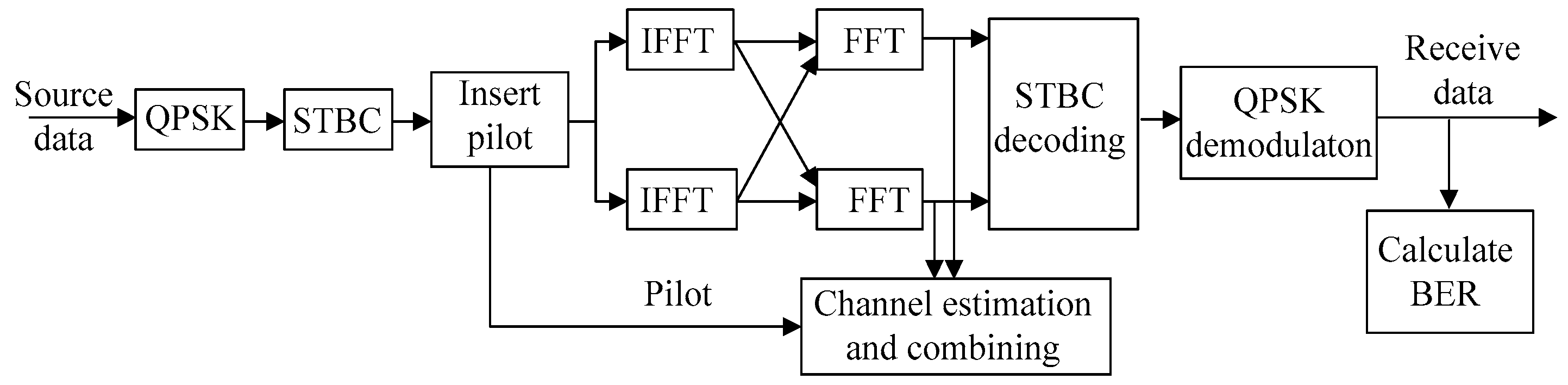
To verify the efficiency of the configuration, a simulation platform is established as shown in Figure 3.
In the simulation model, the channel is designed as a pseudo-static Rayleigh channel in which all of the parameters follow the specification of ITU-R M.1225 for a channel B model [22,23], as listed in Table 1. The MIMO-OFDM system for simulation is constructed to form the scenario in which the number of antennas in the transmitter and receiver are set as NT = 2, NR = 2, respectively, the number of the sub-carrier is configured as N = 128, the length of cyclic prefix (CP) is set to 16; and the sampling cycle is Ts = 2 × 10⁻⁷ s. Quadrature phase shift keying (QPSK) is chosen as the modulation scheme, while the hard decision criteria is adopted for signal detection on the receiver side [21].
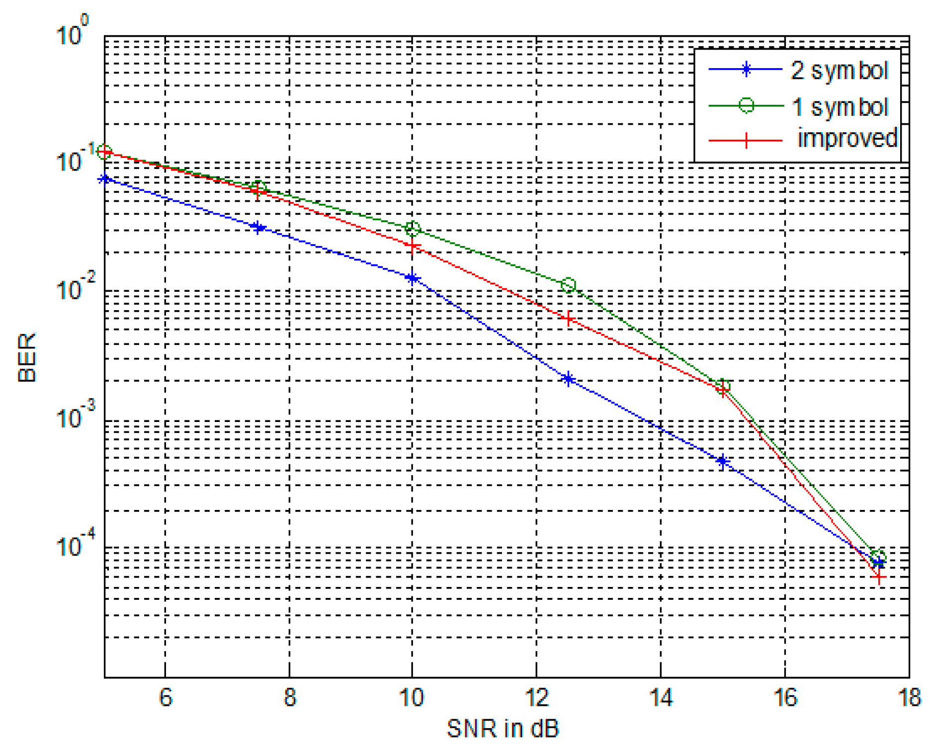
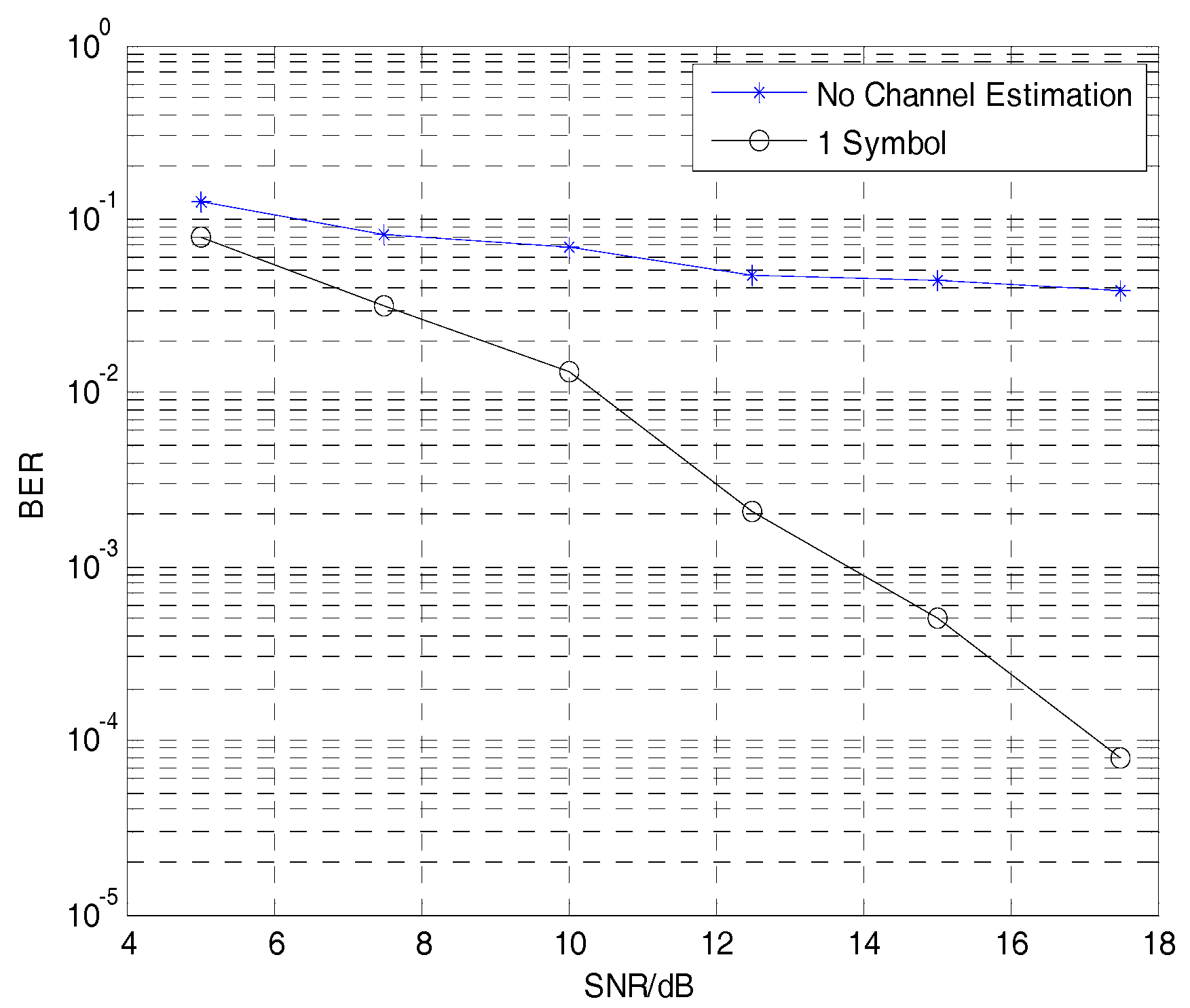
Figure 4 shows the performance of the LS algorithm used for a single-symbol scheme. It can be concluded that the single-symbol scheme, compared with non-channel estimation, can really improve bit error rate (BER), while reducing computation complexity. Figure 5 shows the performance comparison between single-symbol and double-symbol scheme when using two antennas to transmit the same pilot data alternatively within a training block. It can be seen that the double-symbol scheme performs better than the single-symbol scheme for the reason that the double-symbol scheme need not the computation of interpolation so that it avoids interpolation error. However, the double-symbol scheme needs more pilot signals, which increases the system complexity and frequency overhead. The curves of BER versus SNR plotted in Figure 6 correspond to three cases of the single-symbol scheme, double-symbol scheme, and the improved scheme regarding performance trade-off.
The simulation results can be summarized thusly:
- (1)
- Since the number of pilot signals of the double-symbol scheme is four times that of the single-symbol scheme, the interpolation is unnecessary. Thus, the interpolation error can be avoided. From this view, the double symbol-scheme is better than the single-symbol scheme, which has the advantage of more effective overhead.
- (2)
- The tradeoff scheme also does not need interpolation anymore; thus, it is better than the single-symbol scheme. Owing to the number of pilot signals being just half of that in the double-symbol scheme, the performance of tradeoff method is worse than the double-symbol scheme. However, the tradeoff method achieves an optimized balance between system performance and the overhead of the pilot pattern.
6. Conclusions
In this paper, channel estimation in MIMO-OFDM systems is studied on the basis of STBC and LS methods. The performance and overhead comparison are made between the single-symbol scheme and the double-symbol scheme. As a result, an improved pilot scheme, which integrates the features of single- and double-symbol scheme is proposed. Simulation results have shown that the improved scheme can be more effective in achieving a tradeoff between system performance and overhead. It also verifies that, under a certain level of complexity, the performance of channel estimation can be improved through the skilled combination between the optimal pilot scheme and the best criteria of estimation.
Acknowledgments
This work was supported by the National Natural Science Foundation of China (No. 61231017). The authors would like to thank the reviewers and our workmates Kang Xiaofei, Su Yang and Liu Jian for their patience and helpful suggestions on improving the quality of this paper. Without them, the publication of this work is not possible.
Author Contributions
Guomin Li and Guisheng Liao conceived and designed the experiments, analyzed the data; Guomin Li performed the experiments, contributed analysis tools and wrote the paper.
Conflicts of Interest
The authors declare no conflict of interest.
References
- Kang, S.H.; Ha, Y.M.; Joo, E.K. A comparative investigation on channel estimation algorithms for OFDM in mobile communications. IEEE Trans. Broadcast. 2003, 49, 142–149. [Google Scholar] [CrossRef]
- Gui, G.; Xu, L.; Matsushita, S. Improved adaptive sparse channel estimation using mixed square/fourth error criterion. J. Frankl. Inst. 2015, 352, 4579–4594. [Google Scholar] [CrossRef]
- El Ayach, O.; Peters, S.W.; Heath, R.W. The feasibility of interference alignment over measured MIMO-OFDM channels. IEEE Trans. Veh. Technol. 2010, 59, 4309–4321. [Google Scholar] [CrossRef]
- Zhou, P.; Zhao, C.M.; Sheng, B. Channel estimation based on pilot-assisted in the MIMO-OFDM system. J. Electron. Inf. Technol. 2007, 29, 133–137. [Google Scholar]
- Li, Y.G. Simplified channel estimation for OFDM systems with multiple transmit antennas. IEEE Trans. Commun. 2002, 1, 67–75. [Google Scholar]
- Gui, G.; Liu, N.; Xu, L.; Adachi, F. Low-complexity large-scale multiple-input multiple-output channel estimation using affine combination of sparse least mean square filters. IET Commun. 2015, 9, 2168–2175. [Google Scholar] [CrossRef]
- Guo, J.; Wang, D.; Ran, C. Simple channel estimator for STBC-based OFDM systems. IEEE Electron. Lett. 2003, 39, 445–447. [Google Scholar] [CrossRef]
- Zhang, H.; Chen, J.; Tang, Y.; Li, S. Analysis of pilot-symbol aided channel estimation for MIMO-OFDM systems. In Proceedings of the 2004 International Conference on Communications, Circuits and Systems (IEEE Cat. No. 04EX914), Paris, France, 27–29 June 2004; pp. 299–303.
- Van Trees, H.L. Detection, Estimation, and Modulation Theory; John Wiley & Sons: New Jersey, NJ, USA, 2004. [Google Scholar]
- Van de Beek, J.J.; Edfors, O.S.; Sandell, M.; Wilson, S.K.; Börjesson, O.P. On channel estimation in OFDM systems. In Proceedings of the 45th IEEE Vehicular Technology Conference, Chicago, IL, USA, 25–28 July 1995; pp. 815–819.
- Negi, R.; Cioffi, J. Pilot tone selection for channel estimation in a mobile OFDM system. IEEE Trans. Consum. Electron. 1998, 44, 1122–1128. [Google Scholar] [CrossRef]
- Li, G.; Liu, X.; Kang, X.; Liao, G. Improved blind channel estimation for MIMO-OFDM system. J. Appl. Sci. Electron. Inf. Eng. 2016, 34, 286–292. [Google Scholar]
- Sampath, H.; Talwar, S.; Tellado, J.; Erceg, V. A fourth-generation MIMO-OFDM broadband wireless system: Design, performance, and field trial results. IEEE Commun. 2002, 40, 143–149. [Google Scholar] [CrossRef]
- Tong, J.; Gong, Y.H.; Sun, S.X. An adaptive channel tracking method for MIMO-OFDM systems. In Proceedings of the 2004 International Conference on Communications, Circuits and Systems (IEEE Cat. No. 04EX914), Okinawa, Japan, 27–29 June 2004; pp. 354–358.
- Tarokh, V.; Jafarkhani, H. A differential detection scheme for transmit diversity. IEEE Sel. Areas Commun. 2000, 18, 1169–1174. [Google Scholar] [CrossRef]
- Gui, G.; Adachi, F. Stable adaptive sparse filtering algorithms for estimating MIMO channels. IET Commun. 2014, 8, 1032–1040. [Google Scholar] [CrossRef]
- Liang, S.C.; Wu, W.L. Channel Estimation Based on Pilot Subcarrier in Space-Time Block Coded OFDM System. In Proceedings of the International Conference on Communication Technology, Beijing, China, 9–11 April 2003; Volume 2, pp. 1795–1798.
- Mim, H.; Kim, D.I.; Bharagava, V.K. A reduced complexity channel estimation for OFDM systems with transmit diversity in mobile wireless channels. IEEE Trans. Commun. 2002, 50, 799–807. [Google Scholar]
- Lu, X.; Liang, Y.S. STBC pilot channel estimation method based on LS. Commun. Technol. 2009, 41, 63–65. [Google Scholar]
- Wan, F.; Zhu, W.-P. Semiblind sparse channel estimation for MIMO-OFDM system. IEEE Trans. Veh. Technol. 2011, 60, 2569–2582. [Google Scholar] [CrossRef]
- Li, G.; Liao, G. A pilot pattern based algorithm for MIMO-OFDM channel estimation. In Proceedings of the 2016 IEEE International Symposium on Computer, Consumer and Control, Xi’an, China, 4–6 July 2016; pp. 985–989.
- Li, Y.; Zhang, L.; Jia, L. A robust timing synchronization method for OFDM system. In Proceedings of the 2011 Seventh International Conference on Natural Computation, Shanghai, China, 26–28 July 2011; pp. 52–55.
- Li, P.; Wang, P.; Song, Y.; Zhu, T.; Tan, H. Design of correlation-based real-time MIMO channel emulator. Chin. J. Radio Sci. 2015, 30, 929–935. [Google Scholar]
Figure 1.
General procedure of channel estimation.
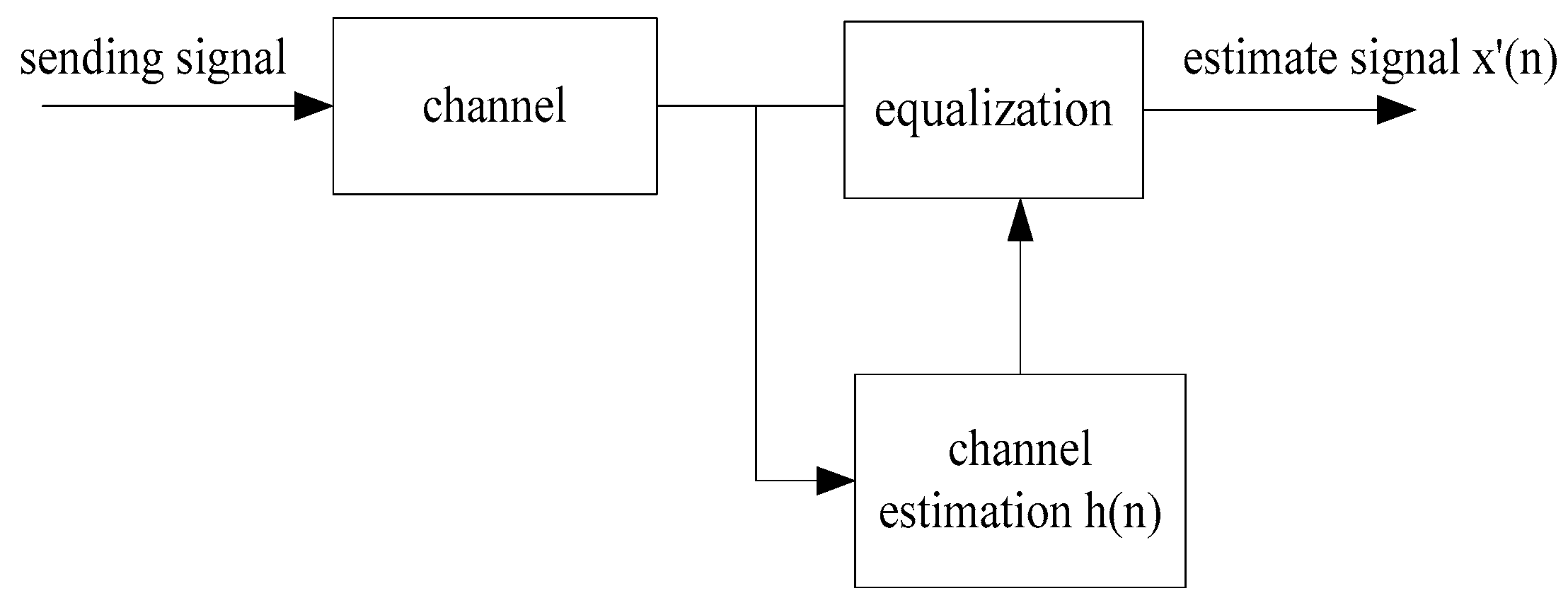
Figure 2.
The architecture of a MIMO-OFDM system.
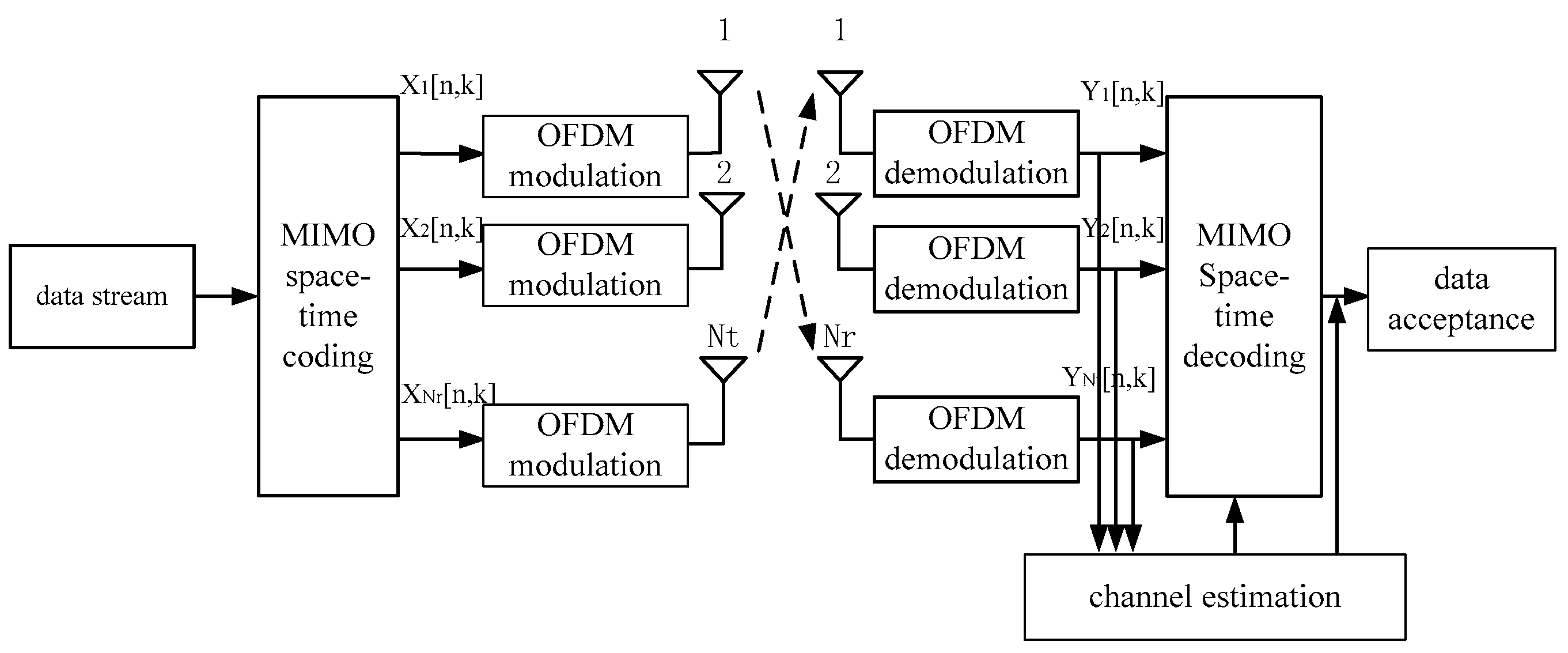
Figure 3.
System simulation platform.

Figure 4.
Performance of channel estimation based on the LS method with one symbol.

Figure 5.
Performance comparison of pilot pattern with one symbol and two symbols.
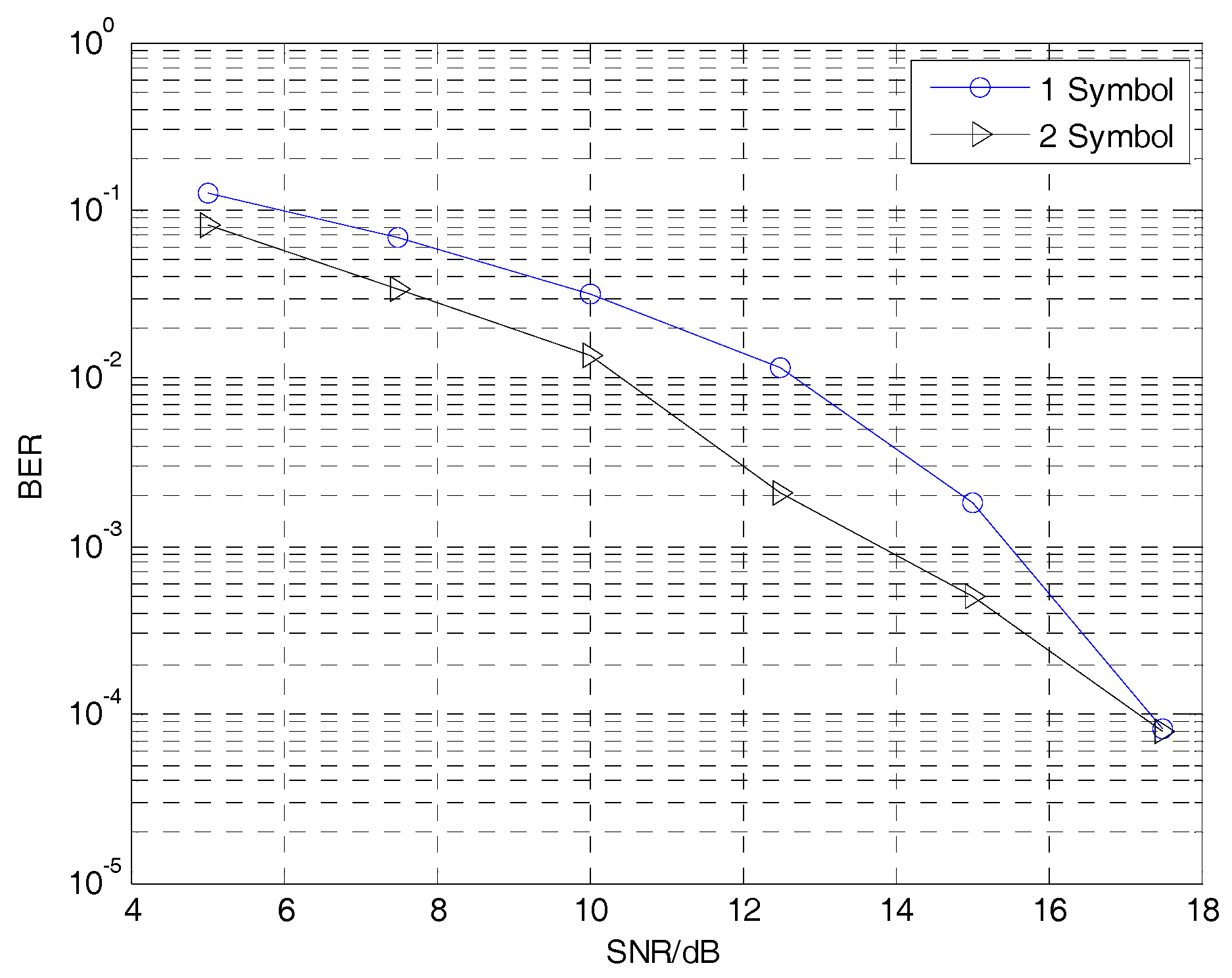
Figure 6.
Performance of channel estimation using a double-symbol pilot pattern.

| Taps | 1 | 2 | 3 | 4 | 5 | 6 |
|---|---|---|---|---|---|---|
| Relative time Delay | 0 | 100 | 200 | 300 | 500 | 700 |
| Average power (dB) | 0 | −3.60 | −7.20 | −10.8 | −18.0 | −25.0 |
© 2016 by the authors. Licensee MDPI, Basel, Switzerland. This article is an open access article distributed under the terms and conditions of the Creative Commons Attribution (CC BY) license ( http://creativecommons.org/licenses/by/4.0/).
Share and Cite
MDPI and ACS Style
Li, G.; Liao, G. A Pilot-Pattern Based Algorithm for MIMO-OFDM Channel Estimation. Algorithms 2017, 10, 3. https://doi.org/10.3390/a10010003
AMA Style
Li G, Liao G. A Pilot-Pattern Based Algorithm for MIMO-OFDM Channel Estimation. Algorithms. 2017; 10(1):3. https://doi.org/10.3390/a10010003
Chicago/Turabian StyleLi, Guomin, and Guisheng Liao. 2017. "A Pilot-Pattern Based Algorithm for MIMO-OFDM Channel Estimation" Algorithms 10, no. 1: 3. https://doi.org/10.3390/a10010003
Note that from the first issue of 2016, this journal uses article numbers instead of page numbers. See further details here.