Expanding the Applicability of Some High Order Househölder-Like Methods

Abstract

This paper is devoted to the semilocal convergence of a Househölder-like method for nonlinear equations. The method includes many of the studied third order iterative methods. In the present study, we use our new idea of restricted convergence domains leading to smaller $\gamma$-parameters, which in turn lead to the following advantages over earlier works (and under the same computational cost): larger convergence domain; tighter error bounds on the distances involved, and at least as precise information on the location of the solution.

1. Introduction

Let $B_1$ and $B_2$ be Banach spaces and D be a non-empty open convex subset of $B_1$. Let also $\mathcal{L}(B_1,B_2)$ stand for the space of bounded linear operators from $B_1$ into $B_2$. In this study, we are concerned with the problem of approximating a locally unique solution $x^{*}$ of the nonlinear equation:

$$F\left(x\right)=0,$$

(1)

where $F:D\subset B_1\to B_2$ is a nonlinear Fréchet-differentiable operator.

Beginning from $t_0$, we can consider different third-order iterative methods to solve the scalar equation $F\left(t\right)=0$, with $F:X\to Y$ and $X=Y=\mathbb{R}$, [1,2].

According to Traub’s classification [3], these third-order methods are divided into two broad classes. On the one hand, the one-point methods, which require the evaluation of F, $F^{\prime }$ and $F^{″}$ at the current point only. For instance,

• The Halley method

  $$t_{n+1}=t_n-\left(\frac{1}{1+\frac{1}{2}{L}_F\left(t_n\right)}\right)\frac{F\left(t_n\right)}{F^{{}^{\prime }}\left(t_n\right)},$$

  where $L_F\left(t\right)=\frac{F\left(t\right)F^{″}\left(t\right)}{F^{\prime }{\left(t\right)}^2}.$
• The Chebyshev method:

  $$t_{n+1}=t_n-\left(1+\frac{1}{2}{L}_F\left(t_n\right)\right)\frac{F\left(t_n\right)}{F^{{}^{\prime }}\left(t_n\right)},$$
• The family of Newton-like methods:

  $$\left\{\begin{array}{c}{\displaystyle t_{n+1}=G\left(t_n\right)=t_n-H\left(L_F\left(t_n\right)\right)\frac{F\left(t_n\right)}{F^{\prime }\left(t_n\right)},n\ge 0,}\hfill \\ {\displaystyle H\left(y\right)=\sum _{j\ge 0}^{}{\tilde{A}}_j{y}^j;{\tilde{A}}_0=1,{\tilde{A}}_1=1/2,{\tilde{A}}_j\in R^{+}\cup \left\{0\right\},\forall j\ge 2,}\hfill \end{array}\right.$$

  (2)

which includes the well-known iterative methods of the third-order Chebyshev, Halley, Super-Halley, Ostrowski and Euler methods.

Notice that the family (2) has the inconvenience of reaching order greater than three only for certain equations. For instance, it is known that the family (2) has fourth order of convergence for quadratic equations, if ${\tilde{A}}_2=1/2$.

On the other hand, the second class is the multipoint methods, which cannot require $F^{″}$. For instance:

Two-step method

$$\begin{array}{rrr}{s}_n& =& t_n-\frac{F\left(t_n\right)}{F^{{}^{\prime }}\left(t_n\right)},\\ t_{n+1}=TS\left(t_n\right)& =& s_n-\frac{F\left(s_n\right)}{F^{{}^{\prime }}\left(t_n\right)}.\end{array}$$

(3)

Notice that this iterative method cannot be included in the family (2). This way, to obtain iterative methods with higher order than three for any function F and to be able to represent some multipoint methods, as (3), we can consider a modification of the family (2) that allow getting this generalization [4]. Therefore, we consider the following family, which includes all of these methods:

$$\begin{array}{ccc}{s}_n\hfill & =\hfill & {\displaystyle t_n-\frac{F\left(t_n\right)}{F^{\prime }\left(t_n\right)},}\hfill \\ t_{n+1}\hfill & =\hfill & {\displaystyle H\left(t_n\right)=s_n-\frac{A_0(F;t_n)}{F^{\prime }\left(t_n\right)}-\left({\displaystyle \sum _{k=2}^{\infty }\frac{A_k(F;t_n)}{F^{\prime }\left(t_n\right)}{\left[\frac{F\left(t_n\right)}{F^{\prime }\left(t_n\right)}\right]}^{k-1}}\right)\frac{F\left(t_n\right)}{F^{\prime }\left(t_n\right)}.}\hfill \end{array}$$

(4)

Notice that (4) is well defined if $|\frac{A_k(F,t)}{F^{\prime }\left(t\right)}|\le k^p,$ for all p and $k\ge 2$ and $|\frac{F\left(t\right)}{F^{\prime }\left(t\right)}|<1$.

Thus, for instance, for $A_0(F;t)=0$ and $A_k(F;t)={\tilde{A}}_{k-1}\frac{F^{\prime \prime }{\left(t\right)}^{k-1}}{F^{\prime }{\left(t\right)}^{k-2}}$, we obtain the previous family (2). On the other hand, if we take $A_k(F;t_n)=0$, for all $k\ge 1$, and:

$$A_0(F;t_n)=F\left(s_n\right),$$

then we get the two-step method (3).

In general, the methods (2) have higher operational cost than the methods (3) when solving a non-linear system. Another measure that takes into account the operational cost that requires an iterative process $\mathsf{\Phi }$ is the computational efficiency given by $CE(\varphi ,F)=o^{\frac{1}{\theta \left(F\right)}}$ where, again, o is the order of convergence of $\mathsf{\Phi }$ and $\theta \left(F\right)$ is the operational cost to apply a step with the iterative process $\mathsf{\Phi }$, that is the number of products needed per iteration and the number of products that appear in the evaluation of the corresponding operator.

Therefore, in order to compare the efficiency of some iterative methods of the new family, we consider the computational efficiency $CE(\mathsf{\Phi },F)$. Note that the methods selected in the family (4) as the most efficient have a lower computational efficiency as more terms in the series are considered.

Notice that, for quadratic equations, the Chebyshev method and the two-step method (method in (7) with $A_0(F;x_n)=F\left(y_n\right)$) have the same algorithm:

$$\begin{array}{ccc}{y}_n\hfill & =\hfill & x_n-F^{{}^{\prime }}{\left(x_n\right)}^{-1}F\left(x_n\right),\hfill \\ x_{n+1}\hfill & =\hfill & y_n-F^{{}^{\prime }}{\left(x_n\right)}^{-1}F\left(y_n\right).\hfill \end{array}$$

(5)

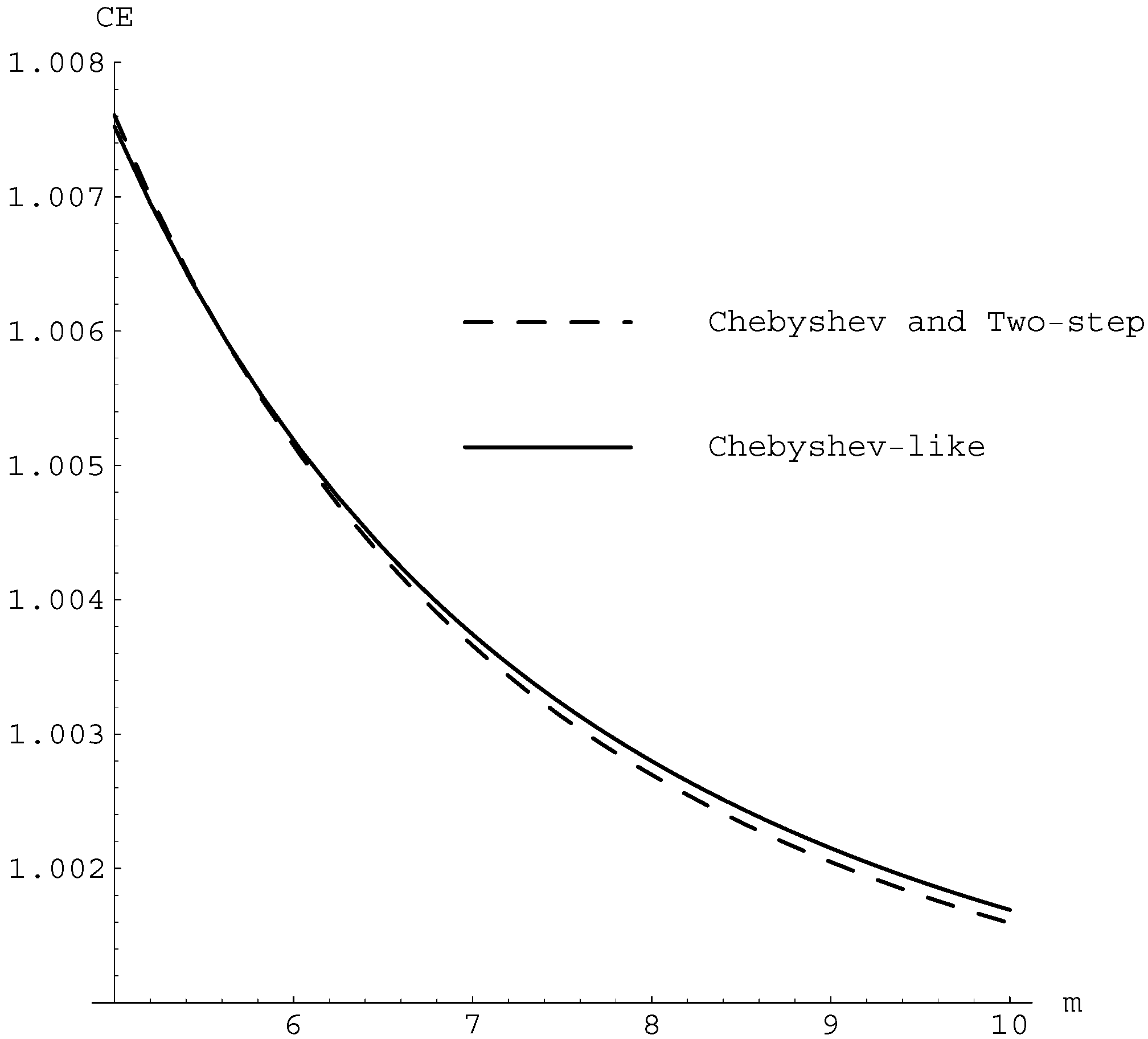
On the other hand, we note that the family of iterative processes (7), with $A_2=1/2$, has the property of having four-order convergence when we consider quadratic equations. Therefore, the iterative process that is more efficient in this family, for quadratic equations, is the known Chebyshev-like method ($A_2=1/2$ and $A_k=0$ for $k\ge 3$ in (7)). Then, we compare this iterative process with the Chebyshev method.

This fourth-order method for quadratic equations can be written as:

$$\begin{array}{ccc}{y}_n\hfill & =\hfill & x_n-F^{{}^{\prime }}{\left(x_n\right)}^{-1}F\left(x_n\right),\hfill \\ z_n\hfill & =\hfill & y_n-F^{{}^{\prime }}{\left(x_n\right)}^{-1}F\left(y_n\right),\hfill \\ x_{n+1}\hfill & =\hfill & z_n-F^{{}^{\prime }}{\left(x_n\right)}^{-1}(2F\left(z_n\right)-C(z_n-y_n)(z_n-x_n)),\hfill \end{array}$$

(6)

For the quadratic equation, the computational efficiency, $CE$, for the Chebyshev method, (5) and (6) methods in the family (7) is $CE=3^{3/(m^3+9m^2+17m)}$, $CE=4^{3/(m^3+12m^2+24m)}$, respectively. As we can observe in Figure 1, the optimum computational efficiency is for the Chebyshev-like method given in (6), when the system has at least six equations.

Recently, in the work by Amat et al. [4], a semilocal convergence analysis was given in a Banach space setting:

$$\begin{array}{ccc}{y}_n\hfill & =\hfill & x_n-{\mathsf{\Gamma }}_{n}F\left(x_n\right),\hfill \\ x_{n+1}\hfill & =\hfill & y_n-{\mathsf{\Gamma }}_n{A}_0(F;x_n)-\left({\displaystyle \sum _{k=2}^{\infty }{\mathsf{\Gamma }}_n{A}_k(F;x_n){\left[{\mathsf{\Gamma }}_{n}F\left(x_n\right)\right]}^{k-1}}\right){\mathsf{\Gamma }}_{n}F\left(x_n\right),\hfill \end{array}$$

(7)

where ${\mathsf{\Gamma }}_n={\left[F^{\prime }\left(x_n\right)\right]}^{-1}$ and the operators $A_k(F;-):D\to \mathcal{L}(\stackrel{(k}{\overbrace{D\times \dots \times D}},B_2)$ are some particular k-linear operators.

An interesting application related to image denoising was presented also in [4]. The approximation, via our family, is of a new nonlinear mathematical model for the denoising of digital images. We are able to find the best method in the family (different of the two-step) for this particular problem. Indeed, the founded method has order four. The denoising model that we propose in this paper permits a good reconstruction of the edges that are the most important visual parts of an image. See also [5,6] for more applications.

On the other hand, the semilocal convergence analysis of method (7) was based on $\gamma$-type conditions [7] that constitute an alternative to the classical Kantorovich-type conditions [8]. The convergence domain for the method (7) is small in general. In the present study, we use our new idea of restricted convergence domains leading to smaller $\gamma$-parameters, which in turn lead to the following advantages over the work in [4] (and under the same computational cost): larger convergence domain; tighter error bounds on the distances involved and an at least as precise information on the location of the solution.

The rest of the paper is organized as follows: the semilocal convergence analysis of the method (7) is given in Section 2, whereas the numerical examples are presented in the concluding Section 3.

2. Semilocal Convergence

We consider Equation (1), where F is a nonlinear operator defined in a non-empty open convex subset D of a Banach space $B_1$ with values in another Banach space $B_2$.

We need the definition of the $\gamma$-condition given in [7].

Definition 1.

Suppose that $F:D\to B_2$ is five-times Fréchet-differentiable. Let $\beta >0$ and $x_0\in D$. We say that F satisfies the γ-condition, if ${\mathsf{\Gamma }}_0=F^{\prime }{\left(x_0\right)}^{-1}\in \mathcal{L}(B_2,B_1)$ and for each $x\in D$:

$$\begin{array}{ccc}\parallel {\mathsf{\Gamma }}_{0}F\left(x_0\right)\parallel \hfill & \le \hfill & \beta ,\hfill \\ \parallel {\mathsf{\Gamma }}_0{F}^{{}^{″}}\left(x_0\right)\parallel \hfill & \le \hfill & {\displaystyle \frac{2\gamma }{(1-\gamma \parallel x-x_0{\parallel )}^2},}\hfill \\ \parallel {\mathsf{\Gamma }}_0{F}^{{}^{″\prime }}\left(x\right)\left|\right|\hfill & \le \hfill & {\displaystyle \frac{6{\gamma }^2}{(1-\gamma \parallel x-x_0{\left|\right|)}^4}=f^{{}^{″\prime }}(\parallel x-x_0\parallel ),}\hfill \\ \parallel {\mathsf{\Gamma }}_0{F}^{\left(iv\right)}\left(x_0\right)\parallel \hfill & \le \hfill & 24{\gamma }^3,\hfill \\ \parallel {\mathsf{\Gamma }}_0{F}^{\left(v\right)}\left(x\right)\parallel \hfill & \le \hfill & {\displaystyle \frac{120{\gamma }^4}{(1-\gamma \parallel x-x_0{\parallel )}^6}=f^{\left(v\right)}(\parallel x-x_0\parallel ),}\hfill \end{array}$$

where:

$$\begin{array}{c}\hfill f\left(t\right)=\beta -t+\frac{\gamma t^2}{1-\gamma t}.\end{array}$$

(8)

Then, the following semilocal convergence result for the method defined in (7) under γ-type conditions was given in [4], Theorem 1:

Theorem 1.

Assume that the operator F satisfies for each $x\in D$:

$$\parallel {\left[F^{\prime }\left(x\right)\right]}^{-1}{A}_k(F;x)\parallel \le k^p,\forall k\ge 2,\dots ,p>0and\parallel {\left[F^{\prime }\left(x\right)\right]}^{-1}F\left(x\right)\parallel <1,$$

(9)

the γ-condition and hypotheses:

$$\begin{array}{c}\alpha \le \beta \gamma \le 3-2\sqrt{2},\hfill \\ A_0(f,t)\ge 0,\left({\displaystyle \sum _{k=2}^{\infty }\frac{A_k(f;t)}{f^{\prime }\left(t\right)}{\left[\frac{f\left(t\right)}{f^{\prime }\left(t\right)}\right]}^{n-1}}\right)\ge 0,\hfill \end{array}$$

(10)

with f given in (30) and $\overline{U}(x_0,R)\subseteq D$, where $R=(1-\frac{1}{\sqrt{2}})\frac{1}{\gamma }$. Then, sequences $\left\{x_n\right\}$, $\left\{y_n\right\}$ generated by the method (7) are well defined in $U(x_0,R)$, remain in $U(x_0,t^{*})$ for each $n=0,1,2\dots$ and converge to a solution $x^{*}\in U(x_0,t^{*})$ of equation $F\left(x\right)=0$, which is unique in $U(x_0,R)$. Moreover, the following estimates hold true for each $n=0,1,2\dots$:

$$\begin{array}{ccc}\parallel y_n-x_n\parallel \hfill & \le \hfill & s_n-t_n,\hfill \\ \parallel x_{n+1}-y_n\parallel \hfill & \le \hfill & t_{n+1}-s_n,\hfill \\ \parallel y_n-x^{*}\parallel \hfill & \le \hfill & t^{*}-s_n,\hfill \\ \parallel x_n-x^{*}\parallel \hfill & \le \hfill & t^{*}-t_n,\hfill \end{array}$$

(11)

where $t_0=0$, $s_0=\beta$,

$$\begin{array}{ccc}\hfill s_n& =& t_n-\frac{f\left(t_n\right)}{f^{\prime }\left(t_n\right)},n\ge 0,\hfill \\ \hfill t_{n+1}& =& {\displaystyle s_n-\frac{A_0(f;t_n)}{f^{\prime }\left(t_n\right)}-\left({\displaystyle \sum _{k=2}^{\infty }\frac{A_k(f;t_n)}{f^{\prime }\left(t_n\right)}{\left[\frac{f\left(t_n\right)}{f^{\prime }\left(t_n\right)}\right]}^{k-1}}\right)\frac{f\left(t_n\right)}{f^{\prime }\left(t_n\right)}.}\hfill \end{array}$$

and:

$$\begin{array}{ccc}\hfill t^{*}& =& \frac{1+\alpha -\sqrt{{(1+\alpha )}^2-8\alpha }}{4\gamma }.\hfill \end{array}$$

Next, we show how to achieve the advantages of our approach as stated in the introduction of this study.

Definition 2.

Let $F:D\to B_2$ be a Fréchet-differentiable operator. Operator F satisfies the center ${\gamma }_0$-Lipschitz condition at $x_0$, if for each $x\in D$:

$$\begin{array}{ccc}\parallel {\mathsf{\Gamma }}_0(F^{\prime }\left(x\right)-F^{\prime }\left(x_0\right))\parallel \hfill & \le \hfill & {\displaystyle \frac{1}{(1-{\gamma }_0\parallel x-x_0{\parallel )}^2}-1.}\hfill \end{array}$$

Remark 1.

Let $D_0:=U(x_0,(1-\frac{1}{\sqrt{2}})\frac{1}{{\gamma }_0})\cap D$. Then, we have that:

$${\displaystyle \parallel {\mathsf{\Gamma }}_0(F^{\prime }\left(x\right)-F^{\prime }\left(x_0\right))\parallel \le \frac{1}{(1-{\gamma }_0\parallel x-x_0{\parallel )}^2}-1<1.}$$

In view of the Banach lemma on invertible operators [8], ${\mathsf{\Gamma }}_0=F^{{}^{\prime }}{\left(x_0\right)}^{-1}\in \mathcal{L}(B_2,B_1)$ and:

$$\parallel {\left[F^{\prime }\left(x\right)\right]}^{-1}{F}^{\prime }\left(x_0\right)\parallel \le {\left({\displaystyle 2-\frac{1}{(1-{\gamma }_0\parallel x-x_0{\parallel )}^2}}\right)}^{-1}.$$

(12)

The corresponding result using the γ-condition given in [7] is:

$$\parallel {\left[F^{\prime }\left(x\right)\right]}^{-1}{F}^{\prime }\left(x_0\right)\parallel \le {\left({\displaystyle 2-\frac{1}{(1-\gamma \parallel x-x_0{\parallel )}^2}}\right)}^{-1}.$$

(13)

for each $x\in D$. However, if $D_0\subseteq D$, then ${\gamma }_0\le \gamma$, so if ${\gamma }_0<\gamma$, the estimate (12) is more precise than (13), leading to more precise majorizing sequences, which in turn lead to the advantages already stated. Indeed, we need the following definition.

Definition 3.

Let $F:D\to B_2$ be a five-times Fréchet-differentiable, which satisfies the center ${\gamma }_0$-condition. We say that operator F satisfies the δ-γ-condition at $x_0$, if for each $x\in D_0$:

$$\begin{array}{ccc}\hfill \parallel {\mathsf{\Gamma }}_{0}F\left(x_0\right)\parallel & \le & \beta ,\hfill \\ \hfill \parallel {\mathsf{\Gamma }}_0{F}^{{}^{″}}\left(x_0\right)\parallel & \le & {\displaystyle \frac{2\delta }{(1-\delta \parallel x-x_0{\parallel )}^2},}\hfill \\ \hfill \parallel {\mathsf{\Gamma }}_0{F}^{{}^{″\prime }}\left(x\right)\left|\right|& \le & {\displaystyle \frac{6{\delta }^2}{(1-\delta \parallel x-x_0{\left|\right|)}^4}=f_1^{{}^{″\prime }}(\parallel x-x_0\parallel ),}\hfill \\ \hfill \parallel {\mathsf{\Gamma }}_0{F}^{\left(iv\right)}\left(x_0\right)\parallel & \le & 24{\delta }^3,\hfill \\ \hfill \parallel {\mathsf{\Gamma }}_0{F}^{\left(v\right)}\left(x\right)\parallel & \le & {\displaystyle \frac{120{\delta }^4}{(1-\delta \parallel x-x_0{\parallel )}^6}=f_1^{\left(v\right)}(\parallel x-x_0\parallel ).}\hfill \end{array}$$

Clearly, we have that $\delta \le \gamma$.

Now, we define the scalar sequences $\left\{{\overline{s}}_n\right\}$, $\left\{{\overline{t}}_n\right\}$ by:

$$\begin{array}{ccc}{\overline{t}}_0& =\hfill & 0,{\overline{s}}_0=\beta ,\hfill \\ {\overline{s}}_n& =\hfill & {\overline{t}}_n-\frac{f_1\left({\overline{t}}_n\right)}{f_1^{\prime }\left({\overline{t}}_n\right)}n\ge 0,\hfill \\ {\overline{t}}_{n+1}& =\hfill & {\displaystyle {\overline{s}}_n-\frac{A_0(f_1;{\overline{t}}_n)}{f_0^{\prime }\left({\overline{t}}_n\right)}-\left({\displaystyle \sum _{k=2}^{\infty }\frac{A_k(f_1;{\overline{t}}_n)}{f_1^{\prime }\left({\overline{t}}_n\right)}{\left[\frac{f_1\left({\overline{t}}_n\right)}{f_1^{\prime }\left({\overline{t}}_n\right)}\right]}^{k-1}}\right)\frac{f_1\left({\overline{t}}_n\right)}{f_1^{\prime }\left({\overline{t}}_n\right)}.}\hfill \end{array}$$

(14)

where function $f_1$ is defined on the interval $[0,1/\delta )$ by:

$$f_1\left(t\right)=\beta -t+\frac{\delta t^2}{1-\delta t},$$

(15)

for some $t\in (0,\frac{1}{\delta })$.

Moreover, define constants ${\alpha }_0$, ${\overline{t}}^{*}$, ${\overline{t}}^{**}$ and $R_0$ by ${\alpha }_0=\delta \beta$, ${\overline{t}}^{*}=\frac{1+{\alpha }_0-\sqrt{{(1+{\alpha }_0)}^2-8{\alpha }_0}}{4\delta }$, ${\overline{t}}^{**}=\frac{1+{\alpha }_0+\sqrt{{(1+{\alpha }_0)}^2-8{\alpha }_0}}{4\delta }$ and $R_0=(1-\frac{1}{\sqrt{2}})\frac{1}{{\gamma }_0}$.

If condition:

$${\alpha }_0\le 3-2\sqrt{2}$$

(16)

holds, then function $f_1$ has two real roots ${\overline{t}}^{*}$ and ${\overline{t}}^{**}$ such that:

$$\beta \le {\overline{t}}^{*}\le \left(1+\frac{1}{\sqrt{2}}\right)\beta \le \left(1-\frac{1}{\sqrt{2}}\right)\frac{1}{\delta }\le {\overline{t}}^{**}\le \frac{1}{2\delta }.$$

Moreover, we have for each $t\in [0,{\overline{t}}^{*})$: $f_1\left(t\right)>0$, $f_1^{\prime }\left(t\right)=\frac{1-2{(1-\delta t)}^2}{{(1-\delta t)}^2}<0$ and:

$$f_1^{\left(i\right)}\left(t\right)=\frac{i!{\delta }^{i-1}}{(1-\delta t)(2+i)},i=2,3,\dots .$$

Notice that:

$$\alpha \le 3-2\sqrt{2}\Rightarrow {\alpha }_0\le 3-2\sqrt{2}$$

(17)

but not necessarily vice versa, unless, if $\gamma =\delta$.

We need a series of auxiliary results.

Lemma 1.

Suppose that ${\alpha }_0\le 3-2\sqrt{2}$, $A_0(f_1;t)\ge 0$ and ${\displaystyle \sum _{k=2}^{\infty }\frac{A_k(f_1;t)}{f_1^{\prime }\left(t\right)}{\left[\frac{f_1\left(t\right)}{f_1^{\prime }\left(t\right)}\right]}^{k-1}\ge 0.}$ Then, sequences $\left\{{\overline{s}}_n\right\}$, $\left\{{\overline{t}}_n\right\}$ generated by (14) are well defined for each $n=0,1,2,\dots$ and converge monotonically to ${\overline{t}}^{*}$ so that:

$$0\le {\overline{t}}_n\le {\overline{s}}_n\le {\overline{t}}_{n+1}<{\overline{t}}^{*}.$$

(18)

Proof. 

Simply replace f, α, $t^{*}$, $s_n$, $t_n$ in the proof of Lemma 2 [4] by $f_1$, ${\alpha }_0$, ${\overline{t}}^{*}$, ${\overline{s}}_n$, ${\overline{t}}_n$, respectively. ☐

Lemma 2.

(a) 

Let $f_1$ be the real function given in (15). Then, the following assertion holds:

$$\begin{array}{c}{f}_1\left({\overline{t}}_{n+1}\right)=\left(\frac{1}{2}{f}_1^{″}\left({\overline{t}}_n\right)\frac{A_0(f_1;{\overline{t}}_n)}{f_1^{\prime }{\left({\overline{t}}_n\right)}^2}-1\right)A_0(f_1;{\overline{t}}_n)\hfill \\ {\displaystyle +f_1^{″}\left({\overline{t}}_n\right)\frac{A_0(f_1;{\overline{t}}_n)}{f_1^{\prime }\left({\overline{t}}_n\right)}\left({\displaystyle 1+\frac{\tilde{h}(f_1;{\overline{t}}_n)}{f_1^{\prime }\left({\overline{t}}_n\right)}}\right)\frac{f_1\left({\overline{t}}_n\right)}{f_1^{\prime }\left({\overline{t}}_n\right)}}\hfill \\ {\displaystyle +\frac{1}{2}{f}_1^{″}\left({\overline{t}}_n\right){\left({\displaystyle \frac{f_1\left({\overline{t}}_n\right)}{f_1^{\prime }\left({\overline{t}}_n\right)}}\right)}^2}\hfill \\ {\displaystyle +\frac{1}{2}{f}_1^{″}\left({\overline{t}}_n\right){\left({\displaystyle \frac{\tilde{h}(f_1;{\overline{t}}_n)f_1\left({\overline{t}}_n\right)}{f_1^{\prime }\left({\overline{t}}_n\right)}}\right)}^2}\hfill \\ {\displaystyle +\left({\displaystyle \frac{f_1^{\prime \prime }\left({\overline{t}}_n\right)f_1\left({\overline{t}}_n\right)}{f_1^{\prime }{\left({\overline{t}}_n\right)}^2}-1}\right)\frac{\tilde{h}(f_1;{\overline{t}}_n)f_1\left({\overline{t}}_n\right)}{f_1^{\prime }\left({\overline{t}}_n\right)}}\hfill \\ {\displaystyle +{\int }_{{\overline{t}}_n}^{{\overline{t}}_{n+1}}{f}_1^{‴}\left(t\right)({\overline{t}}_{n+1}-t)dt,}\hfill \end{array}$$

where:

$${\displaystyle \tilde{h}(f_1;{\overline{t}}_n)=\sum _{k=2}^{\infty }\frac{A_k(f_1;{\overline{t}}_n)}{f_1^{\prime }\left(t_n\right)}{\left[\frac{f_1\left({\overline{t}}_n\right)}{f_1^{\prime }\left({\overline{t}}_n\right)}\right]}^{k-1}}$$

and $A_k(f_1;-):\mathbb{R}\to \mathbb{R}$ are real differentiable functions.

(b) 

If F has a continuous third-order Fréchet-derivative on D, then the following assertion holds:

$$\begin{array}{c}F\left(x_{n+1}\right)=\left(\frac{1}{2}{F}^{″}\left(x_n\right){\mathsf{\Gamma }}_n{A}_0(F;x_n){\mathsf{\Gamma }}_n-I\right)A_0(F;x_n)\hfill \\ +F^{″}\left(x_n\right){\mathsf{\Gamma }}_n{A}_0(F;x_n)\left(I+{\mathsf{\Gamma }}_n\tilde{H}(F;x_n)\right){\mathsf{\Gamma }}_{n}F\left(x_n\right)\hfill \\ +\frac{1}{2}{F}^{″}\left(x_n\right){\mathsf{\Gamma }}_{n}F\left(x_n\right){\mathsf{\Gamma }}_{n}F\left(x_n\right)\hfill \\ +\frac{1}{2}{F}^{″}\left(x_n\right){\left({\mathsf{\Gamma }}_n\tilde{H}(F;x_n){\mathsf{\Gamma }}_{n}F\left(x_n\right)\right)}^2\hfill \\ +\left(F^{″}\left(x_n\right){\mathsf{\Gamma }}_{n}F\left(x_n\right){\mathsf{\Gamma }}_n-I\right)\tilde{H}(F;x_n){\mathsf{\Gamma }}_{n}F\left(x_n\right)\hfill \\ {\displaystyle +{\int }_{x_n}^{x_{n+1}}{F}^{‴}\left(x\right)(x_{n+1}-x)dx,}\hfill \end{array}$$

where:

$${\displaystyle \tilde{H}(F;x_n)=\sum _{k=2}^{\infty }{A}_k(F;x_n){\left({\mathsf{\Gamma }}_{n}F\left(x_n\right)\right)}^{k-1}}$$

and $A_k(F;-):D\to \mathcal{L}(\stackrel{(k}{\overbrace{D\times \dots \times D}},Y)$ are some particular k-linear operators.

(c) 

$\parallel {\mathsf{\Gamma }}_{0}F\left(x_{n+1}\right)\parallel \le f_1\left(t\right)\left({\overline{t}}_{n+1}\right)$.

Proof. 

(a)

Simply use function $f_1$ instead of f in the proof of Lemma 3 in [4].

(b)

The same with Lemma 5 in [4].

(c)

Use $f_1$ instead of f in Lemma 5 [4].

 ☐

Lemma 3.

Suppose F satisfies the ${\gamma }_0$-center-condition on D and the δ-γ-condition on $D_0$. Then, the following items hold:

(a) 

$F^{\prime }{\left(x\right)}^{-1}\in \mathcal{L}(Y,X)$ and:

$$\parallel F^{\prime }{\left(x\right)}^{-1}{F}^{\prime }\left(x_0\right)\parallel \le -\frac{1}{f_0^{\prime }(\parallel x-x_0\parallel )},foreachx\in D$$

where:

$$f_0\left(t\right)=b-t+\frac{{\gamma }_0{t}^2}{1-{\gamma }_{0}t}$$

(b) 

$\parallel {\mathsf{\Gamma }}_0{F}^{(m-1)}\left(x\right)\parallel \le f_1^{(m-1)}(\parallel x-x_0\parallel ),m=3orm=5.$

Proof. 

(a)

See Remark 1.

(b)

Simply replace function f by $f_1$ in Lemma 4 in [4].

 ☐

Lemma 4.

Suppose F satisfies the γ-condition on D. Then, the following items hold:

(a) 

F satisfies the ${\gamma }_0$-condition on D and the δ-γ-condition on $D_0$;

(b) 

${\gamma }_0\le \gamma$;

(c) 

$\delta \le \gamma$;

Moreover, if $\alpha \le 3-2\sqrt{2}$, then ${\overline{\alpha }}_0=b_0\gamma \le 3-2\sqrt{2}$, ${\alpha }_0\le 3-2\sqrt{2}$,

$$\parallel F^{\prime }{\left(x\right)}^{-1}{F}^{\prime }\left(x_0\right)\parallel \le -\frac{1}{f_0^{\prime }(\parallel x-x_0\parallel )}\le -\frac{1}{f^{\prime }(\parallel x-x_0\parallel )},$$

and:

$$\parallel {\mathsf{\Gamma }}_0{F}^{\prime }\left(x_0\right)\parallel \le -\frac{1}{f_1^{\prime }(\parallel x-x_0\parallel )}\le -\frac{1}{f^{\prime }(\parallel x-x_0\parallel )}.$$

Furthermore, (15) supposes that ${\gamma }_0\le \delta$ and from (18); we have:

$$\parallel F^{\prime }{\left(x\right)}^{-1}{F}^{\prime }\left(x_0\right)\parallel \le -\frac{1}{f_0^{\prime }(\parallel x-x_0\parallel )}\le -\frac{1}{f_1^{\prime }(\parallel x-x_0\parallel )}.$$

Proof. 

The assertions hold from Lemma 3, (18), the definition of functions $f_0$, $f_1$, f and the definition of ${\gamma }_0$, γ and δ-condition. ☐

Theorem 2.

Suppose that the operator F satisfies the conditions of Lemma 1, 2, 3, (9), (18), and $A_0(f_1;t)>=0$ hold. Then, sequences $\left\{x_n\right\}$, $\left\{y_n\right\}$, generated by the method (7) are well defined in $U(x_0,{\overline{t}}^{*})$, remain in $\overline{U}(x_0,{\overline{t}}^{*})$ for each $n=0,1,2,\dots ,$ and converge to a solution ${\overline{x}}^{*}\in \overline{U}(x_0,{\overline{t}}^{*})$ of equation $F\left(x\right)=0$. The limit point ${\overline{x}}^{*}$ is the only solution of equation $F\left(x\right)=0$ in $U(x_0,R_0)$. Moreover, the following estimates are true for each $n=0,1,2,\dots$:

$$\begin{array}{c}\parallel y_n-x_n\parallel \le {\overline{s}}_n-{\overline{t}}_n,\hfill \\ \parallel x_{n+1}-y_n\parallel \le {\overline{t}}_{n+1}-{\overline{s}}_n,\hfill \\ \parallel y_n-x^{*}\parallel \le {\overline{t}}^{*}-{\overline{s}}_n,\hfill \\ \parallel x_n-x^{*}\parallel \le {\overline{t}}^{*}-t_n,\hfill \end{array}$$

(19)

where ${\overline{t}}^{*}={lim}_n{\overline{t}}_n.$

Proof. 

We shall show the estimates (19). Using mathematical induction as a consequence of the following recurrence relations:

($M_k^1$)

$x_k\in \overline{U}(x_0,{\overline{t}}_k)$;

($M_k^2$)

$\parallel F^{\prime }{\left(x_k\right)}^{-1}{F}^{\prime }\left(x_0\right)\parallel \le -\frac{1}{f_0^{\prime }\left({\overline{t}}_k\right)}\le -\frac{1}{f_1^{\prime }\left({\overline{t}}_k\right)}$;

($M_k^3$)

$\parallel y_k-x_k\parallel \le {\overline{s}}_k-{\overline{t}}_k$;

($M_k^4$)

$y_k\in \overline{U}(x_0,{\overline{s}}_k)$;

($M_k^5$)

$\parallel x_{k+1}-x_k\parallel \le {\overline{t}}_{k+1}-{\overline{s}}_k$.

Items ($M_0^i$), $i=1,2,3,4,5$ are true by the initial conditions. Suppose ($M_k^i$) are true for $k=0,1,\dots ,n$. Then, we shall show that they hold for $n+1$. We have in turn that:

$$\begin{array}{ccc}\parallel x_{k+1}-x_0\parallel \hfill & \le \hfill & \parallel x_{k+1}-y_k\parallel +\parallel y_k-x_k\parallel +\parallel x_k-x_0\parallel \hfill \\ \hfill & \le \hfill & ({\overline{t}}_{k+1}-{\overline{s}}_k)+({\overline{s}}_k-{\overline{t}}_{k+1})+({\overline{t}}_{k+1}-{\overline{t}}_0)={\overline{t}}_{k+1},\hfill \end{array}$$

so ($M_{k+1}^1$) is true. By Lemma 4 and condition ${\gamma }_0\le \delta$, we get that ${\mathsf{\Gamma }}_{k+1}\in \mathcal{L}(Y,X)$ and:

$$\parallel {\mathsf{\Gamma }}_{k+1}{F}^{\prime }\left(x_0\right)\parallel \le -\frac{1}{f_0^{\prime }(\parallel x_{k+1}-x_0\parallel }\le -\frac{1}{f_0^{\prime }\left({\overline{t}}_{k+1}\right)}\le -\frac{1}{f_1^{\prime }\left({\overline{t}}_{k+1}\right)},$$

so ($M_{k+1}^2$) is true. By Lemma 2, we obtain in turn that ${\mathsf{\Gamma }}_{k+1}\in \mathcal{L}(Y,X)$ and:

$$\parallel {\mathsf{\Gamma }}_0{F}^{\prime }\left(x_{k+1}\right)\parallel \le f_1^{\prime }\left({\overline{t}}_{k+1}\right),$$

so:

$$\begin{array}{ccc}\parallel y_{k+1}-x_{k+1}\parallel \hfill & =\hfill & \parallel -{\mathsf{\Gamma }}_{k+1}F\left(x_{k+1}\right)\parallel \le \parallel {\mathsf{\Gamma }}_{k+1}{F}^{\prime }\left(x_0\right)\parallel \parallel {\mathsf{\Gamma }}_{0}F\left(x_{k+1}\right)\parallel \hfill \\ \hfill & \le \hfill & -\frac{f_1^{\prime }\left({\overline{t}}_{k+1}\right)}{f_1^{\prime }\left({\overline{t}}_{k+1}\right)}={\overline{s}}_{k+1}-{\overline{t}}_{k+1},\hfill \end{array}$$

$$\begin{array}{ccc}\parallel y_{k+1}-x_0\parallel \hfill & \le \hfill & \parallel y_{k+1}-x_k\parallel +\parallel x_k-y_{k-1}\parallel +\parallel y_{k-1}-x_{k-1}\parallel +\parallel x_{k-1}-x_0\parallel \hfill \\ \hfill & \le \hfill & ({\overline{s}}_{k+1}-{\overline{t}}_k)+({\overline{t}}_k-{\overline{s}}_{k-1})+({\overline{s}}_{k-1}-{\overline{t}}_{k-1})+({\overline{t}}_{k-1}-{\overline{t}}_0)={\overline{s}}_{k+1},\hfill \end{array}$$

and:

$$\parallel x_{k+1}-y_k\parallel \le \parallel \frac{1}{2}{L}_F\left(x_k\right)\sum _{k=3}^{\infty }{\mathsf{\Gamma }}_k{A}_k(F;x_k){\left({\mathsf{\Gamma }}_{k}F\left(x_k\right)\right)}^{k-1}\parallel \parallel y_k-x_k\parallel \le {\overline{t}}_{k+1}-{\overline{t}}_k,$$

so ($M_{k+1}^4$) and ($M_{k+1}^5$) are also true, which completes the induction. ☐

Remark 2.

We have so far weakened the sufficient semilocal convergence conditions of the method (7) (see (17)) and have also extended the uniqueness of the solution ball from $U(x_0,R)$ to $U(x_0,R_0)$, since for ${\gamma }_0<\gamma$, we have that $R<R_0$. It is worth noticing that these advantages are obtained under the same computational cost, since in practice, the computation of constant γ requires the computation of constants ${\gamma }_0$ and δ as special cases.

Next, it follows by a simple inductive argument and the definition of the majorizing sequences that the error bounds on the distances $\parallel x_{n+1}-x_n\parallel$, $\parallel x_{n+1}-y_n\parallel$, $\parallel x_n-y_n\parallel$, $\parallel y_{n+1}-y_n\parallel$, $\parallel x_n-x^{*}\parallel$ and $\parallel y_n-x^{*}\parallel$ can be improved. In particular, we have:

Proposition 1.

Under the hypotheses of Theorem 2 and Lemma 4, further suppose that for each $u,u_1,u_2,v,v_1,v_2\in [0,R]$, the following hold:

$$\begin{array}{ccc}\hfill {\displaystyle u-\frac{f_1\left(u\right)}{f_1^{\prime }\left(u\right)}}& \le & {\displaystyle v-\frac{f\left(v\right)}{f^{\prime }\left(v\right)},foru\le v,}\hfill \\ \hfill {\displaystyle -\frac{f_1\left(u\right)}{f_1^{\prime }\left(u\right)}}& \le & {\displaystyle -\frac{f\left(v\right)}{f^{\prime }\left(v\right)},foru\le v,}\hfill \\ \hfill u_1-g_1\left(u_2\right)& \le & v_1-g\left(u_2\right),for{u}_1\le v_1,u_2\le v_2,u_1\le u_2,v_1\le v_2,\hfill \\ \hfill g_1\left(u\right)& \le & g\left(v\right),foru\le v,\hfill \end{array}$$

(20)

where functions g and $g_1$ are defined by:

$$g\left(t\right)=\frac{A_0(f,t)}{f^{\prime }\left(t\right)}+\left({\displaystyle \sum _{k=2}^{\infty }\frac{A_k(f;t)}{f^{\prime }\left(t\right)}{\left[\frac{f\left(t\right)}{f^{\prime }\left(t\right)}\right]}^{k-1}}\right)\frac{f\left(t\right)}{f^{\prime }\left(t\right)}$$

and:

$$g_1\left(t\right)=\frac{A_0(f_1,t)}{f_1^{\prime }\left(t\right)}+\left({\displaystyle \sum _{k=2}^{\infty }\frac{A_k(f_1;t)}{f_1^{\prime }\left(t\right)}{\left[\frac{f_1\left(t\right)}{f_1^{\prime }\left(t\right)}\right]}^{k-1}}\right)\frac{f_1\left(t\right)}{f_1^{\prime }\left(t\right)}$$

Then, the following estimates hold:

$${\overline{s}}_n\le s_n,$$

(21)

$${\overline{s}}_n-{\overline{t}}_n\le s_n-t_n,$$

(22)

$${\overline{t}}_{n+1}\le t_{n+1},$$

(23)

$${\overline{t}}_{n+1}-{\overline{s}}_n\le t_{n+1}-s_n,$$

(24)

$${\overline{t}}^{*}\le t^{*}.$$

(25)

Proof. 

Estimates (21), (22) and (23) follow using a simple inductive argument from conditions given in (20) Moreover, the estimate (25) follows by letting $n\to \infty$ in the estimate (21). ☐

Remark 3.

Clearly, under the hypotheses of Proposition 1, the error bounds on the distances are at least as tight, and the information on the location of the solution $x^{*}$ is at least as precise with the new technique.

The result of Theorem and Proposition 1 can be improved further, if we use another approach to compute the upper bounds on the norms $\parallel {\mathsf{\Gamma }}_k{F}^{\prime }\left(x_0\right)\parallel$.

Definition 4.

Suppose that there exists $L_0>0$ such that the center-Lipschitz condition is satisfies:

$$\parallel {\mathsf{\Gamma }}_0(F^{\prime }\left(x\right)-F^{\prime }\left(x_0\right))\parallel \le L_0\parallel x-x_0\parallel$$

(26)

for each $x\in D$ holds. Define $D_0^{*}=D\cup U(x_0,\frac{1}{L_0})$.

Then, we have that:

$$\parallel {\mathsf{\Gamma }}_0(F^{\prime }\left(x\right)-F^{\prime }\left(x_0\right))\parallel \le L_0\parallel x-x_0\parallel <1,$$

so $F^{\prime }{\left(x\right)}^{-1}\in \mathcal{L}(Y,X)$ and:

$$\parallel F^{\prime }{\left(x\right)}^{-1}{F}^{\prime }\left(x_0\right)\parallel \le \frac{1}{1-L_0\parallel x-x_0\parallel }=-{\overline{f}}_0^{\prime }(\parallel x-x_0{\parallel )}^{-1},$$

(27)

where ${\overline{f}}_0\left(t\right)=\frac{L_0}{2}{t}^2-t+\beta .$ Estimate (27) is more precise than (12) if:

$${\overline{f}}_0^{\prime }\left(t\right)\le f_0^{\prime }\left(t\right),\mathrm{for}\mathrm{each}t\in [0,\rho ],$$

(28)

where $\rho =min\{\frac{1}{L_0},R_0\}$. If

$$\frac{1}{L_0}<R_0,$$

(29)

then $D_0^{*}$ is a strict subset of D. This leads to the construction of an at least as tight function $f_2$ as $f_1$.

Definition 5.

Let $F:D\to B_2$ be five-times Fréchet-differentiable, which satisfies the center-Lipschitz condition (26). We say that the operator F satisfies the λ-γ-condition at $x_0$, if for each $x\in D_0^{*}$:

$$\begin{array}{ccc}\parallel {\mathsf{\Gamma }}_{0}F\left(x_0\right)\parallel \hfill & \le \hfill & \beta ,\hfill \\ \parallel {\mathsf{\Gamma }}_0{F}^{{}^{″}}\left(x_0\right)\parallel \hfill & \le \hfill & {\displaystyle \frac{2\lambda }{(1-\lambda \parallel x-x_0{\parallel )}^2},}\hfill \\ \parallel {\mathsf{\Gamma }}_0{F}^{{}^{″\prime }}\left(x\right)\left|\right|\hfill & \le \hfill & {\displaystyle \frac{6{\lambda }^2}{(1-\lambda \parallel x-x_0{\left|\right|)}^4}=f_2^{{}^{″\prime }}(\parallel x-x_0\parallel ),}\hfill \\ \parallel {\mathsf{\Gamma }}_0{F}^{\left(iv\right)}\left(x_0\right)\parallel \hfill & \le \hfill & 24{\lambda }^3,\hfill \\ \parallel {\mathsf{\Gamma }}_0{F}^{\left(v\right)}\left(x\right)\parallel \hfill & \le \hfill & {\displaystyle \frac{120{\lambda }^4}{(1-\lambda \parallel x-x_0{\parallel )}^6}=f_2^{\left(v\right)}(\parallel x-x_0\parallel ),}\hfill \end{array}$$

where function $f_2$ is defined on the interval $[0,\frac{1}{\lambda })$ by:

$$f_2\left(t\right)=\beta -t+\frac{\lambda t^2}{1-\lambda t}.$$

(30)

Define scalar sequences $\left\{{\overline{\overline{t}}}_n\right\}$, $\left\{{\overline{\overline{s}}}_n\right\}$, points ${\overline{\overline{t}}}^{*}$, ${\overline{\overline{t}}}^{**}$ as, $\left\{{\overline{t}}_n\right\}$, $\left\{{\overline{s}}_n\right\}$, points ${\overline{t}}^{*}$, ${\overline{t}}^{**}$, respectively, by replacing function $f_1$ by $f_2$, and suppose:

$${\alpha }_0^{*}:=\lambda \beta \le 3-2\sqrt{2}.$$

We have by (29) that:

$$\lambda \le \delta$$

so:

$${\alpha }_0\le 3-2\sqrt{2}\Rightarrow {\alpha }_0^{*}\le 3-2\sqrt{2}.$$

Then, with above changes, the condition (28) also replacing the condition in Lemma 3 $\left(a\right)$ and the center-Lipschitz condition (26) replacing the ${\gamma }_0$-center gamma condition, we can recover the results after Definition 4 until Remark 3 in this setting.

3. Concluding Remarks

The results obtained so far in this paper are based on the idea of restricted convergence domains, where the gamma constants (or Lipschitz constants) and consequently the corresponding sufficient semilocal convergence conditions, majorizing functions and sequences are determined by considering the set $D_0$ (or $D_0^{*}$), which can be a strict subset of the set D on which the operator F is defined. This way, one expects (see also the numerical examples) that the new constants will be at least as small as the ones in [4] leading to the advantages as already stated before. The smaller the subset of D is containing the iterates $\left\{x_n\right\}$ of the method (7), the tighter the constants are. When constructing such sets (see, e.g., $D_0$ or $D_0^{*}$), it is desirable if possible not to add hypotheses, but to stay with the same information. Otherwise, the comparison between old and new results will not be fair. Looking in this direction, we can improve our results also, if we simply redefine sets $D_0$ and $D_0^{*}$, respectively, as follows:

$${\tilde{D}}_0=D\cup U(y_0,{\tilde{R}}_0)$$

and:

$${\tilde{D}}_0^{*}=D\cup U(y_0,\frac{1}{L_0}-\beta ),$$

where:

$${\tilde{R}}_0={\overline{R}}_0-\beta$$

Notice that ${\tilde{D}}_0\subseteq D_0\subseteq D$ and ${\tilde{D}}_0^{*}\subset D_0^{*}\subseteq D$. Clearly, the preceding results can be rewritten with ${\tilde{D}}_0$ (or ${\tilde{D}}_0^{*}$) replacing $D_0$ (or $D_0^{*}$). These results will be at least as good as the ones using $D_0$ (or $D_0^{*}$), since the constants will be at least as tight. Notice:

(a)

We are still using the same information, since $y_0$ is defined by the second sub-step of the method (7) for $n=0$, i.e., it depends on the initial data $(x_0,F)$

(b)

The iterates $\left\{x_n\right\}$ lie in ${\tilde{D}}_0$ (or ${\tilde{D}}_0^{*}$), which is an at least as precise a location as $D_0$ (or $D_0^{*}$). Moreover, the solution $x^{*}\in U(y_0,{\tilde{R}}_0)$ (or $x^{*}\in U(y_0,\frac{1}{L_0}-\beta )$), which is a more precise location than $U(x_0,R_0)$ (or $U(x_0,\frac{1}{L_0})$).

Finally, the results can be improved further as follows:

• Case related to the center ${\gamma }_0$-condition (see Definition 2): Suppose that there exists ${\beta }_1\ge 0$ such that:

  $$\parallel x_1-y_0\parallel \le {\beta }_1$$

  and:

  $$\beta +{\beta }_1<R_0.$$

  Then, there exists $t_1$ such that:

  $$\beta +{\beta }_1<t_1<R_0.$$

  Define the set ${\tilde{\tilde{D}}}_0$ by:

  $${\tilde{\tilde{D}}}_0:=D\cup U(x_1,t_1).$$

  Then, we clearly have that:

  $${\tilde{\tilde{D}}}_0\subseteq {\tilde{D}}_0\subseteq D_0.$$

  Suppose the conditions of Definition 4 hold, but on the set ${\tilde{\tilde{D}}}_0$. Then, these conditions will hold for some parameter $\overline{\delta }$ and function $\overline{f_1}$, which shall be at least as tight as δ, $f_1$, respectively. In particular, the sufficient convergence conditions shall be:

  $${\overline{\alpha }}_0=\overline{\delta }\beta \le 3-2\sqrt{2}$$

  and:

  $${\alpha }_0\le 3-2\sqrt{2}\Rightarrow {\alpha }_0^{*}\le 3-2\sqrt{2}\Rightarrow {\overline{\alpha }}_0\le 3-2\sqrt{2}.$$

  The majorizing sequences $\left\{{\kappa }_n\right\}$, $\left\{{\mu }_n\right\}$ shall be defined:

  $${\kappa }_0=0,{\mu }_0=\beta ,{\kappa }_1=\beta +{\beta }_1,{\mu }_1=\beta ,$$

  and $\left\{{\kappa }_n\right\}$, $\left\{{\mu }_m\right\}$, $m=1,2\dots ,n=2,\dots$ as sequences $\left\{{\overline{\overline{s}}}_n\right\}$, $\left\{{\overline{\overline{t}}}_n\right\}$, but with ${\overline{f}}_1$ replacing function $f_1$. Then, the conclusions of Theorem 2 will hold in this setting. Notice that the estimate $\parallel x_1-y_0\parallel \le {\beta }_1$ still uses the initial data as $\parallel y_0-x_0\parallel \le {\beta }_1.$
• Case related to the center-Lipschitz condition (26): Similarly, to the previous case, but:

  $${\tilde{\tilde{D}}}_0^{*}:=D\cup U(x_1,t_1).$$

  Then, again, we have that:

  $${\tilde{\tilde{D}}}_0\subseteq {\tilde{D}}_0^{*}\subseteq D_0^{*}.$$
• An example:
  Let us consider $X=Y={\mathbb{R}}^3$, $D=U(0,1)$, $x^{*}=(0,0,0)$ and the nonlinear operator $F(x,y,z)=(e^x-1,\frac{e-1}{2}{y}^2+y,z)$.
  In this case, we can consider ${\gamma }_0=\frac{(e-1)}{2}<\gamma =\frac{e}{2}$, [9].

References

- Chun, C. Construction of third-order modifications of Newton’s method. Appl. Math. Comput. 2007, 189, 662–668. [Google Scholar] [CrossRef]
- Ezquerro, J.A.; Gutiérrez, J.M.; Hernández, M.A.; Salanova, M.A. Chebyshev-like methods and quadratic equations. Rev. Anal. Numer. Theor. Approx. 1999, 28, 23–35. [Google Scholar]
- Traub, J.F. Iterative Methods for the Solution of Equations; Prentice-Hall: Englewood Cliffs, NJ, USA, 1964. [Google Scholar]
- Amat, S.; Hernández, M.A.; Romero, N. On a family of high-order iterative methods under gamma conditions with applications in denoising. Numer. Math. 2014, 127, 201–221. [Google Scholar] [CrossRef]
- Amat, S.; Hernández, M.A.; Romero, N. Semilocal convergence of a sixth order iterative method for quadratic equations. Appl. Numer. Math. 2012, 62, 833–841. [Google Scholar] [CrossRef]
- Amat, S.; Hernández, M.A.; Romero, N. A modified Chebyshev’s iterative method with at least sixth order of convergence. Appl. Math. Comput. 2008, 206, 164–174. [Google Scholar] [CrossRef]
- Argyros, I.K. An inverse free Newton-Jarrat-type iterative method for solving equations under gamma condition. J. Appl. Math. Comput. 2008, 28, 15–28. [Google Scholar] [CrossRef]
- Kantorovich, L.V.; Akilov, G.P. Functional Analysis; Pergamon Press: Oxford, UK, 1982. [Google Scholar]
- Argyros, I.K.; Hilout, S.; Khattri, S.K. Expanding the applicability of Newton’s method using Smale’s theory. J. Appl. Math. Comput. 2014, 261, 183–200. [Google Scholar] [CrossRef]
© 2017 by the authors. Licensee MDPI, Basel, Switzerland. This article is an open access article distributed under the terms and conditions of the Creative Commons Attribution (CC BY) license (http://creativecommons.org/licenses/by/4.0/).
Share and Cite
MDPI and ACS Style
Amat, S.; Argyros, I.K.; Hernández-Verón, M.A.; Romero, N. Expanding the Applicability of Some High Order Househölder-Like Methods. Algorithms 2017, 10, 64. https://doi.org/10.3390/a10020064
AMA Style
Amat S, Argyros IK, Hernández-Verón MA, Romero N. Expanding the Applicability of Some High Order Househölder-Like Methods. Algorithms. 2017; 10(2):64. https://doi.org/10.3390/a10020064
Chicago/Turabian StyleAmat, Sergio, Ioannis K. Argyros, Miguel A. Hernández-Verón, and Natalia Romero. 2017. "Expanding the Applicability of Some High Order Househölder-Like Methods" Algorithms 10, no. 2: 64. https://doi.org/10.3390/a10020064
Note that from the first issue of 2016, this journal uses article numbers instead of page numbers. See further details here.