A Monarch Butterfly Optimization for the Dynamic Vehicle Routing Problem


Department of Information Science and Technology, Dalian Maritime University, Dalian 116026, China
*
Authors to whom correspondence should be addressed.
Algorithms 2017, 10(3), 107; https://doi.org/10.3390/a10030107
Submission received: 29 June 2017
/
Revised: 4 September 2017
/
Accepted: 4 September 2017
/
Published: 12 September 2017
Abstract
:The dynamic vehicle routing problem (DVRP) is a variant of the Vehicle Routing Problem (VRP) in which customers appear dynamically. The objective is to determine a set of routes that minimizes the total travel distance. In this paper, we propose a monarch butterfly optimization (MBO) algorithm to solve DVRPs, utilizing a greedy strategy. Both migration operation and the butterfly adjusting operator only accept the offspring of butterfly individuals that have better fitness than their parents. To improve performance, a later perturbation procedure is implemented, to maintain a balance between global diversification and local intensification. The computational results indicate that the proposed technique outperforms the existing approaches in the literature for average performance by at least 9.38%. In addition, 12 new best solutions were found. This shows that this proposed technique consistently produces high-quality solutions and outperforms other published heuristics for the DVRP.
1. Introduction
The dynamic vehicle routing problem (DVRP) is a hard combinatorial optimization problem which is advanced by information and communication technologies that allow information to be obtained and processed in real time, typically used in distribution logistics and transportation systems. This system facilitates quick updating of transportation system plans in unexpected or uncertain events, for example if roads between two customers are blocked off, customers can modify their orders, or when the travel time for some routes is increased due to bad weather conditions or traffic congestion, etc. On the other hand, customers in the e-market place increasingly expect quicker and more flexible fulfilment of their transportation requests. In this context, the DVRP is becoming increasingly interesting and important.
The DVRP is a variant of the VRP—the well-known NP-hard problem which is used in general cases. Because VRPs can be regarded as special cases of dynamic VRPs, dynamic VRPs are at least as hard as VRPs; therefore, research efforts mainly focus on metaheuristics and intelligent optimization algorithms. For example, Ismail [1] designed a hybrid GA and Tabu Search heuristic to solve the DVRP. Oliveira et al. [2] applied ant colony system (ACS) techniques to solve the DVRP with time window constraints and a capacitated fleet. Belfiore and Yoshizaki [3] proposed a scatter search (SS) approach to deal with real-life heterogeneous fleet vehicle routing with time windows and split deliveries in Brazil. Chen and Xu [4] proposed a dynamic column generation algorithm for the DVRP with time windows. de Armas et al. [5] presented a general variable neighborhood search algorithm to solve a real-world application of the DVRP.
In this paper, a monarch butterfly optimization (MBO) approach is proposed for the DVRP. Although MBO has been successfully applied to a great variety of hard combinatorial optimization problems ([6,7,8,9]), this paper, as far as we know, proposes the first MBO-based algorithm for the DVRP.
Biologically-inspired computation is a field focusing on the development of computational tools, modeled on the principles that exist in natural systems. The results presented in recent publications show that bio-inspired approaches are now highly competitive with other state-of-the-art heuristics.
MBO was proposed by Wang et al. [10] in 2015. Preliminary studies indicated that MBO is a very competitive metaheuristic algorithm [10], when compared with ant colony optimization (ACO) [11], biogeography-based optimization (BBO) [12] and differential evolution (DE) [13], is very easy to implement because it only needs to fine-tune migration and adjusting operators. In addition, MBO is very capable of finding the shortest paths [9]. However, MBO may fail to reach optimal performance on average and standard values in certain test cases [10].
This paper considers a version of the DVRP in which some of the customers’ locations and associated demands are unknown at the start of the working day and arrive gradually as time passes. All vehicles start from the depot to serve yesterday’s remaining customers after opening time and must return to the depot by the closing time. A similar problem was first introduced by Kilby et al. [14]. In order to overcome the MBO shortcoming, a greedy algorithm is incorporated into the migration operation and butterfly adjusting operator, and a later perturbation procedure is applied after the butterfly adjusting operator, to maintain a balance between global diversification and local intensification. To the best of our knowledge, this is the first MBO implementation for the DVRP. It is tested using data sets introduced in Kilby et al. [14] and Montemanni et al. [15], and compared to other well-known meta-heuristics. As a result, we obtain an average gap of −9.38%, provide 12 new best solutions from 21 instances, and improve the overall performance for this set of instances.
The remainder of this paper is organized as follows: In Section 2, we define the DVRP model tackled here and present a literature review of the existing papers that deal with the DVRP. Section 3 contains a description of our algorithm. In Section 4, we include the results of the experiment and the corresponding analysis to test our proposed algorithm. We summarize the major conclusions of this article in Section 5.
2. Dynamic Vehicle Routing Problem (DVRP)
2.1. Problem Description
To allow better understanding of the DVRP, Figure 1 shows a simple example of a dynamic vehicle routing problem. In the example, two uncapacitated vehicles must service both advance- and immediate-request customers. The static customers are represented by white nodes, while those that are immediate requests are depicted by black nodes. The dashed lines represent the two routes that the dispatcher has planned prior to the vehicles leaving the depot (Figure 1A). The two dash-dotted lines indicate the vehicle positions at the time the dynamic requests appear. Ideally, the dispatcher routes should be adjusted to fulfill the dynamic customers’ requests (Figure 1B). Finally, the vehicles deliver the demands of all customers and return to the depot (Figure 1C).
The study problem concerns routing a fleet of capacitated vehicles in real time to deliver goods ordered by a partially-known set of customers. There is a fleet of K homogenous vehicles, each with an identical capacity (Q), and a set of n customers {1, 2, …, n} is considered. The problem can be modeled by an undirected graph, G = (V, E), where V is a vertex set and E is an edge set (V = {0}∪S∪D, and E = {(i, j) | i, j ∈ V, i < j}). Vertex 0 denotes a depot, which has a working time from e0 to l0 (0 ≤ e0 < l0). C is a set of customers (requests) to be serviced. For each customer, (I ∈ S∪D), there is a location (xi, yi), a demand of goods (di), an appearance moment (ai (e0 ≤ ai ≤ l0)), and a service time (si). At the same time, each edge is defined by a non-negative distance (cij) and the travel time (tij) between all customers’ locations. For DVRPs, there are two sets of customers: S and D. S is composed of static customers, who are known from an earlier working day, and D includes all dynamic customers, who appear with time. A solution, S, is composed of a set of routes satisfying all customers’ demands once. Each route (Rk ∈ S) starts and ends at the depot, and does not exceed the vehicle capacity (Q). A route consists of a sequence of customers to visit (Rk = {0, …, j, …, 0}), where j ∈ V denotes the j-th customer. For each customer (I ∈ Rk), wi is the vehicle’s waiting time, and the vehicle’s arriving time (bi) should satisfy bi = bi−1 + si−1 + wi−1 + ti−1,i (b0 = e0), when we reversely calculate the latest arrival time with zi = zi+1 − ti+1,i − si (zj+1 = l0).
Similar to [14], we also divide a working day (T) into time slices (nts), each with an equal length of time (T/nts, where T = l0 − e0), where TS = {TS1, TS2, …, TSts}. Each time slice represents a partial static VRP, where TS1 only includes static customers in S. The equation TS\TS1 considers the customers received at the previous time slice and those who have not been visited yet.
Hence, two decision variables, xijk and yik, are defined as follows:
xijk = 1 if the edge (i, j) is visited by vehicle k and 0 in all other cases.
yik = 1 if customer i is visited by vehicle k and 0 in all other cases.
The general mathematical model for DVRP is described as follows:
s.t.
The objective (1) is to minimize the total distance travelled during each time slice. Expression (2) ensures that during each time slice, each vehicle does not exceed its capacity. Expressions (3)–(6) ensure that each customer, apart from the depot, is visited once, and only once, by one vehicle, during each time slice. The Expression (7) ensures that all vehicles start from the depot during initialization and return to the depot at the end of the route. Meanwhile, the number of vehicles out in use cannot exceed the total quantity at the depot. Expression (8) is the travel time constraints, because every vehicle must return to the depot before the closing time.
2.2. Related Work
The Dynamic Vehicle Routing Problem (DVRP) with capacity and time duration constraints was introduced by Kilby et al. [14] and further refined by Montemanni et al. [15]. These authors proposed some benchmark instances for the DVRP and presented a study on how the degree-of-dynamism affects the final travel costs. Montemanni et al. [15], who extended Kilby et al.’s work [14], considered a DVRP as an extension to the standard VRP, by decomposing a DVRP as a sequence of static VRPs, and then solving them using an ACS algorithm. Other optimization techniques have been applied. Khouadjia et al. [16] presented particle swarm optimization. Yang et al. [17] proposed a hybrid large neighborhood search. In a recent survey, Pillac et al. [18] classified routing problems from the perspective of information quality and evolution. They introduced the notion of degree of dynamism, and presented a comprehensive review of applications and solution methods for dynamic vehicle routing problems. Bekta et al. [19] provided another survey in this area, which provided a deeper and more detailed analysis. Last but not least, Psaraftis et al. [20] shed more light into work in this area, over more than 3 decades, by developing a taxonomy of DVRP papers according to 11 criteria.
Along with advances in technology, improvements to problem-solving methods have been made in order to interact with dynamic environments, and to combine fast responses with quality solutions. Based on the quality of information, Pillac et al. [18] classified DVRPs into two categories: deterministic and stochastic. The present work falls under the deterministic category, for which approaches are based on periodic or continuous re-optimization.
Periodic re-optimization approaches typically commence at the beginning of the day, with an initial optimization that produces an initial set of routes; then the solution is re-optimized either whenever the available information changes, or at a fixed re-optimization interval. Chen and Xu [4] proposed a dynamic, column generation approach for solving a DVRP, with hard time windows, in which all requests need to be serviced. The authors used the concept of decision epochs over the planning horizon, which indicate the moments of the day when the re-optimization process is executed. Montemanni et al. [15] employed an ACS to solve the dynamic VRP by dividing the overall planning horizon into periods (time slices), as in Kilby et al. [14]. During each time slice, a static problem is solved by considering all requests known at the beginning of this time slice. A similar approach was also employed by Elhassania et al. [21], Euchi et al. [22] and Mańdziuk and Żychowski [23].
In contrast, continuous re-optimization approaches commence at the beginning of operations with an initial set of routes, and the vehicles are informed only about their next destination. It keeps high quality solutions within an adaptive memory. A decision procedure is used to update the solutions in the adaptive memory whenever the available information is updated. Updates typically occur due to either a new dynamic customer request service, or the vehicle reaches a customer. Gendreau et al. [24] were the first to employ continuous re-optimization. These authors proposed a Tabu Search heuristic to address the DVRP arising in a long-distance courier service, in which time windows could be violated at some cost. The approach keeps a pool of good solutions in its adaptive memory, which is used to generate initial solutions for a parallel Tabu Search. Whenever a new customer request arrives, it is checked against all the solutions from the adaptive memory to decide whether it should be accepted or rejected. A fast local search procedure is then applied to select the best solution. When the vehicle reaches a customer, the solution is also updated in the adaptive memory and the next destination of the vehicle is identified, based on the best solution. In another study, Bent and Van Hentenryck [25] generalized this framework and introduced the concept of the multiple plan approach to solve the DVRP. The method attempts to continuously generate different solutions based on static and known dynamic customers. A solution pool (routing plans) is used to generate an appropriate solution. When a new customer arrives, a procedure checks if they can be served or not. If they can be served, the customer request is inserted into the solution pool and incompatible solutions are discarded. The solution pool is updated during each event in order to ensure that all solutions are consistent with the current state of the system.
3. The Proposed Algorithm for DVRP
We used the periodic re-optimization strategy to solve the DVRP. This strategy has been used in many DVRP works, such as Kilby et al. [14] and Montemanni et al. [15]. The basic idea of the strategy is to divide a DVRP into a series of static VRPs for every time-slice. The initial states of the static VRPs are different from standard static VRPs—that is, vehicles start from their position in the last slice.
The modified MBO algorithm we propose includes three important parts: (1) an insert heuristic to place new requests into the current solution at the end of each time slice; (2) a greedy strategy, incorporated into the standard MBO, which accepts only the monarch butterfly individuals that have better fitness than their parents, and (3) a subsequent perturbation (2-opt*) to increase the search diversity and the chance of escaping local optima. Next, we discuss the proposed algorithm in detail.
3.1. Solution Representation
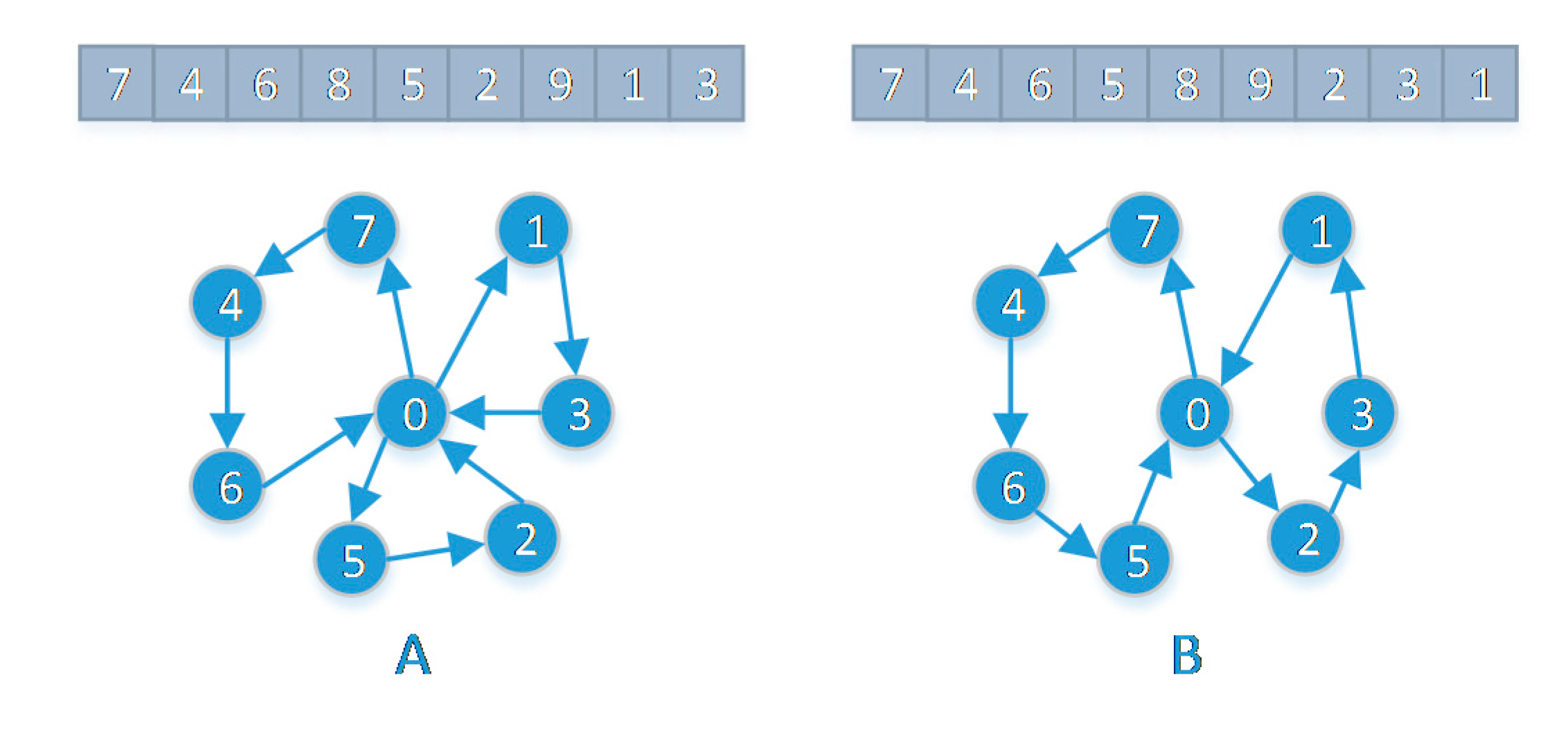
The representation used in our work is dedicated to the DVRP. We propose a simple and intuitionistic natural number encode which expresses the route of k vehicles to the n customers they serve. As previously described, 0 represents the depot, and 1, 2, …, n refers to each customer. As the total number of vehicles is k, the maximum route distribution is also k. Each route begins with the depot, and ends with the depot. In order to reflect the distribution route in coding, we increase k − 1 to represent the virtual depots, respectively expressed as n + 1, …, n + k − 1. A non-duplication of a random arrangement of the natural numbers—1, 2, …, n, n + 1, …, n + k − 1—constitutes an individual.
An example of butterfly representation and its decoding are presented in Figure 2. There are seven customers and three vehicles to complete the task of distribution; we use a non-duplication of a random arrangement of the natural numbers—1, 2, …, 9 (among them, 8 and 9 are virtual depots)—to represent the distribution routes. In Figure 1A, an individual (7 4 6 8 5 2 9 1 3) contains three distribution routes (route 1: 0-4-6-0, route 2: 0-5-2-0, and route 3: 0-1-3-0), while in Figure 2B, an individual (7 4 6 5 8 9 2 3 1) corresponds to the program of the distribution path, route 1: 0-7-4-6-5-0, route 2: 0-2-3-1-0—a total of two distribution routes.
3.2. Initial Population
In accordance with Kilby et al. [14] and many similar works, a working day is split into nts equal-length time slices, and in each time slice a static VRP is solved, with the aim of servicing the known customers so far. We postpone the arrival of a new request to the end of the current time slice and optimize the next time slice. So, a cut-off time (Tco), is considered, as introduced in Montemanni et al. [15], which postpones orders after Tco to the next working day. In addition, an advanced commitment time, (Tac), is also employed to allow a driver to respond to new orders prior to the time of processing the order itself. The first partial static VRP created at the beginning of the working day (T1) consists of all static customers which are left over from the previous working day, as defined by the Tco parameter. We apply a random approach to generate an initial feasible solution (S). Initially, S consists of k − 1 virtual depots, and then we try to update those routes by inserting customers randomly. This process is repeated until all customers have been assigned to a route. Each individual is defined as a random permutation of these known customers and existing routes. Hence, at each slice, all butterflies have the same length and contain the same numbers (customers’ and vehicles’ identifiers). All butterflies will be verified against the capacity and feasibility rules described above.
The next static problem considers all orders received during the previous time slice as well as those which have not been visited by drivers yet. In our simulation, each vehicle (k) starts from the location of the last visited customer (i), with a departure time (dti) corresponding to the end of the service time for this customer (dti = bi + si), and with a remaining capacity equal to the capacity left after serving all previously visited customers.
A decision to wait or go occurs when a vehicle finishes servicing a customer. The algorithm must choose between keeping the vehicle waiting at its current location or beginning to move towards the next customer. Assume that in l-th time slice (TSl), the vehicle (k) has finished serving the customer (i) and is ready to serve the next customer (I + 1) in the route (Rk). If it satisfies the inequalities (9), the vehicle will wait at the customer until Tl (Tl = l*T/nts), and the wait time (wi) at the customer is defined in Equation (10)
3.3. Monarch Butterfly Optimization (MBO)
MBO is a new naturally-inspired metaheuristic algorithm, which is proposed by Wang et al. [10] in 2015. It is inspired by the behavior of the monarch butterfly during migration. In MBO, all the monarch butterfly individuals are idealized and located in two lands only: northern USA and southern Canada (Land 1) and Mexico (Land 2). Accordingly, the positions of the monarch butterflies are updated in two ways: the migration operator and the butterfly adjusting operator. In the following subsections, we discuss our modified operations for solving the DVRPs.
3.3.1. Migration Operator
The migration operator is designed to update the monarch butterfly migration between Land 1 and Land 2, on which monarch butterflies make up subpopulations 1 and 2 respectively. At first, the number of monarch butterflies in Lands 1 and 2 can be considered as NP1 = ceil(p*NP) and NP2 = NP − NP1, respectively, where NP is the total number of monarch butterflies, p is the ratio of monarch butterflies in Land 1, and ceil(x) rounds x to the nearest integer greater than or equal to x. Accordingly, migration operator can be formulated as
where . represents the kth element of xi at generation t + 1. Similarly, . indicates the kth element of xr1 at generation t, and . represents the kth element of xr2 at generation t. The current generation number is represented by t. Monarch butterflies (r1 and r2) are selected randomly from subpopulation 1 and subpopulation 2. The condition variable (r) is calculated as
where peri indicates the migration period and is set to 1.2 in the basic MBO method [10] and rand is a random number derived from a uniform distribution.
r = rand * peri
3.3.2. Butterfly Adjusting Operator
This operator is used to update the positions of the monarch butterflies in subpopulation 2. It can be updated as follows:
where represents the kth element of xj at generation t + 1; indicates the kth element of xbest at generation t, which represents the best location of the monarch butterflies in Lands 1 and 2; and represents the kth element of xr3 at generation t; the monarch butterfly r3 is selected randomly from subpopulation 2. If rand > p, there has another step. The position of the butterfly is further updated using Levy flight, if rand > BAR:
where the variable BAR is the butterfly adjusting rate. If BAR is smaller than a random value, the kth element of xj at generation t + 1 is updated, where α is the weighting factor, as shown in Equation (15).
where Smax is the maximum walk step. In Equation (14), dx is the walk step of butterfly j that can be calculated by Levy flight.
3.4. Greedy Acceptance
In the basic MBO method, all the newly-generated butterflies are accepted, and are kept in the next generation, while a greedy strategy is used to only accept the butterfly individuals that have better fitness in our algorithm. This greedy strategy can be formulated as follows:
where is a newly-generated butterfly individual for the next generation. The terms and are the fitness levels of butterfly and , respectively.
3.5. Later Perturbation
In order to enhance the ability of escaping from a local optimum, we employ a perturbation method to increase the search diversity. We randomly select an individual from the population, and then apply the later perturbation to improve the selected solution. If the resultant solution is feasible, it replaces the worst individual in the population.
The later perturbation uses two improving procedures, as illustrated in Figure 3. First, we use a 2-opt heuristic, which inverts sequences of one single route; second, we use a 2-opt* heuristic, which exchanges the ending segments of two different routes. A first improvement strategy is used, which means that the local search restarts immediately when an improvement is found. Each local search runs until no more improvements are possible. The 2-opt local search runs first, its output solution being the input to the 2-opt* local search. The local search terminates when no 2-opt* move exists that can further improve the solution.
3.6. Algorithm Structure
The modified MBO is shown in Algorithm 1. At first, all parameters are initialized. The variable nts divides the working day (T) into equal time slices. For each time slice, the following procedure is repeated: dynamic customers arriving at time slice TSl are added to the request pool (U) (Line 4). Specially, for TS1, U only stores all static customers. For other time slices, the location of each vehicle is updated by Equations (9) and (10) with the current best solution (S). Then, the unvisited customers from S are removed and inserted into U (Lines 5–8). The population (P) of NP (=|U|) individuals is initialized. Next, the basic MBO is repeated. First, the population is divided into two subpopulations, according to their fitness values, in which subpopulation 1 includes NP1 better individuals and subpopulation 2 includes the rest. Afterwards, an offspring of subpopulation 1 is generated, using the migration operator (Lines 14–19). Then, individuals of subpopulation 2 are updated by the butterfly adjusting operator (Lines 20–25). Note that each two operators only accept the butterfly individuals that have better fitness (Lines 18 and 24). Next, offspring of the two subpopulations are regrouped into one population. Finally, later perturbations are applied to local search for any one individual. The current best individual is used as an input in the next time slice. The above procedure is repeated until the termination condition is satisfied.
| Algorithm 1 MBODVRP |
|
4. Experimental Results
In this section, some computational results are presented, in order to evaluate the performance of the improved MBO described in Section 3. We carried out extensive experiments on relevant benchmarks. We first introduce the benchmarks instances and the parameter settings for the experiments. We then show the results, along with a comparative analysis, on several public data sets derived from Montemanni et al. [15] and Kilby et al. [14].
In order to evaluate the performance of the proposed algorithm, we implemented the algorithm in Visual C# under Windows Server 2012 R2 Standard on a PC with Intel® Xeon® E5-2620 @ 2.40 GHz CPU and 16 GB RAM.
4.1. Benchmarks Description
Our experimental results are based on the benchmarks proposed by Kilby et al. [14] and extended by Monemanni et al. [15]. They were derived from publicly available VRP benchmark data from three separate VRP sources (datasets). The first dataset consists of 12 instances, varying from 75 to 150 customers, taken from Taillard et al. [26]. The second dataset consists of seven instances, with sizes varying from 50 to 199 customers, derived from Christofides et al. [27]. The third set consists of two instances, with sizes varying from 71 to 134 customers, derived from Fisher et al. [28]. The number of customers can be inferred from the name of each instance. The service area may consist of uniformly distributed customers, clustered customers, or a combination of both. In order to obtain dynamic problems, Kilby et al. [14] added the concept of length of the working day into to these problem, and gave each instance an appearance time which signifies when the order becomes available (during the working day) and a duration, namely the time required to perform an order once it reaches the customer. They also fixed the number of available vehicles to 50 for each problem. More details can be found in Kilby et al. [14].
In order to compare our results with existing algorithms, a number of parameters needed to be adjusted. The first was nts, the number of time slices in the optimization. In Montemanni et al. [15], it was found that setting the parameter to nts = 25 yielded the best trade-off between the objective value and computational cost. Secondly, the advanced commitment time (Tac) was set at 0. Finally, the cutoff time (Tco), was set to 0.5T, where T is the total length of the working day. In particular, for each time slice, we limited computation time to 30 s. Then, T equals 30 × 25 = 750 s for the entire simulation.
4.2. Comparison with the Literature for DVRP
A comparison for the quality of the solution, in terms of minimizing travel distances, was done between our approach and other metaheuristics proposed previously in the literature. In order to obtain significant results, our approach was executed five times for each instance. Table 1 and Table 2 show the best computational results by our MBO algorithm and the average results over five runs, respectively. There are six columns in Table 1 and Table 2: the instance, our MBO algorithm, the best known solutions (BKS), the algorithm to find the BKS, the relative error (RE) (i.e., RE = (MBO − BKS)/BKS × 100%) and the computational time by MBO (note that we cannot compare with other algorithms as there is no such data available in the public domain or in the literature). There are other best and average results in Table 1 and Table 2 provided by some heuristic algorithms as follows: GA2007 and TS by Hanshar and Ombuki-Berman [29], DAPSO and VNS by [16], GA2014 by [21], HLNS by [17] and AAC-2OPT by [22].
As you can see, our approach is very competitive. Table 1 shows that MBO found 12 out of 21 new best solutions, compared to the BKS. The average distance of all instances by the MBO was 2096.55 which is lower than the BKS’s average cost of 2163.70. It made an improvement of 1.12% over the BKS. Regarding the computation time of MBO, the longest was no more than 470.15 s (much lower than the time limit of 750 s that we set), and the shortest was 42.44 s, while the average time for each instance was 168.18 s. In particular, the computation time for each time slice was only 6.73 s on average. This indicates that MBO has good computational capability.
From Table 2, our average results were superior to GRASP in almost all instances, and better than BKS in 14 instances. All these results allow us to say that our MBO is effective and shows the viability to generate very high quality solutions for the DVRP.
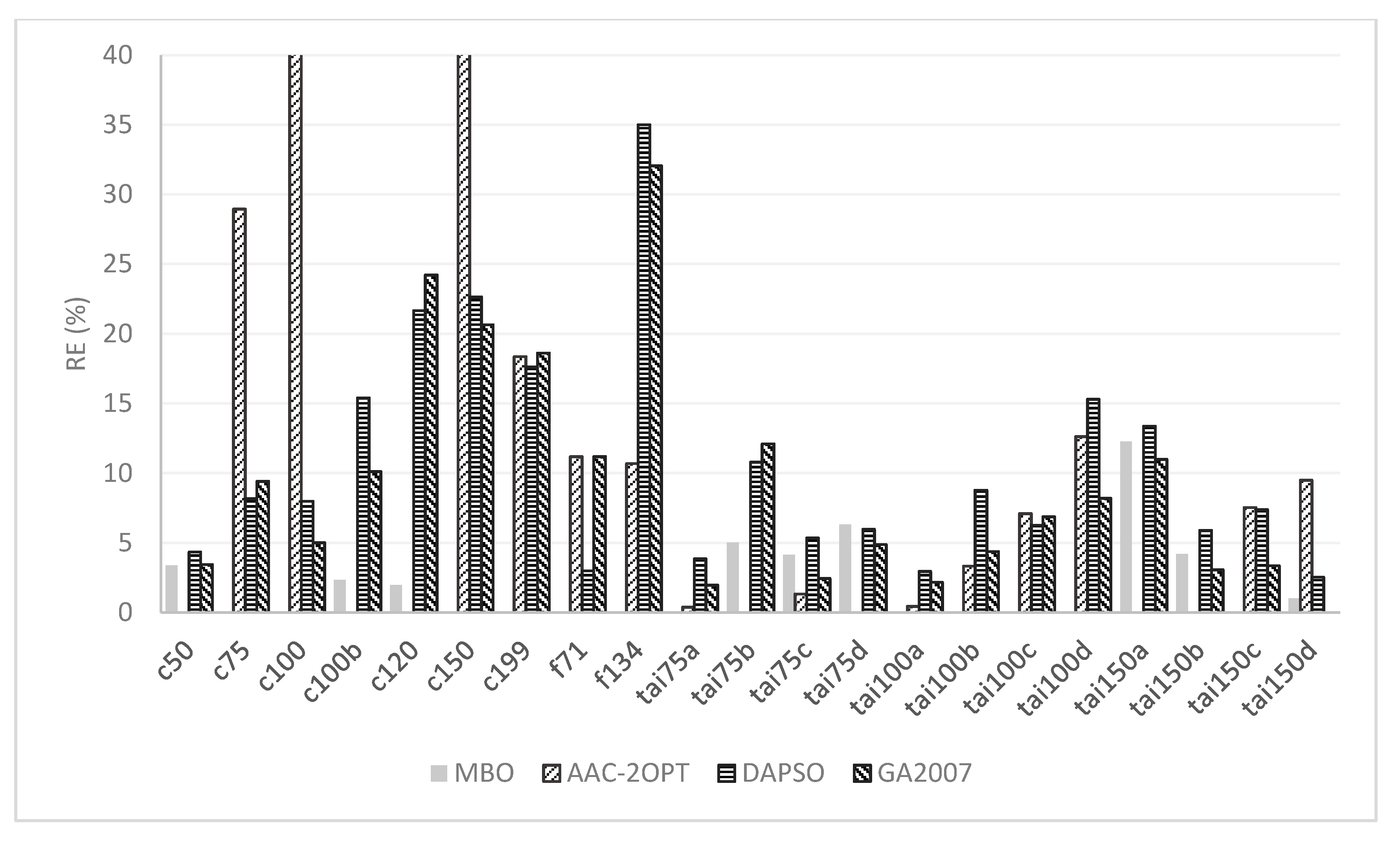
In the next experiment, we compared the AAC-2OPT, DAPSO, and GA2007 with our MBO. The percentage of deviation from the known optimal solution concerning problems can be seen as a chart in Figure 4. It shows that MBO is superior to other methods. The deviation of MBO is less than 5% for all instances except tail75d and tail150a.
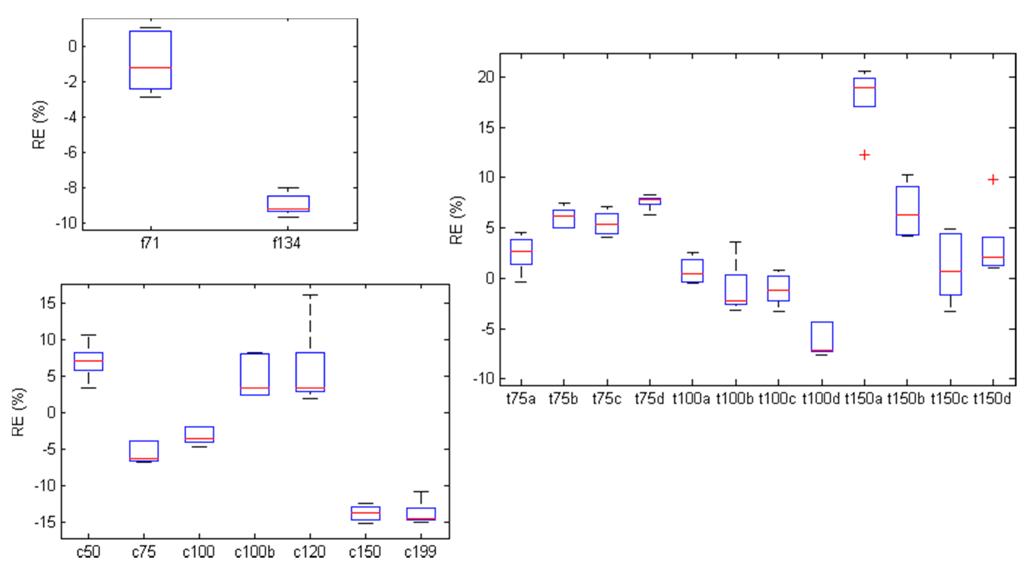
In this experiment, we analyzed the results in detail. Figure 5 shows, for each data set, the dispersion diagrams of the solutions found by our approach. Note that the solution values are presented as the relative error from the BKS.
In most cases, our MBO gets a relative error of no greater than 10% from the BKS, and central values tend to be between 0 and 5%. It is interesting to note that the quality and stability of the solutions are not size dependent. In particular, f134, c75, c100, c150, c199, and t100d have instances with less than 5% relative error. This means those instances are better than the BKS.
5. Conclusions
This paper studied the DVRP, a method where the customers appear dynamically, and which requires a combination of the vehicles’ current states and the customers’ current information to re-plan routes. In this paper, an MBO approach, called MBO–DVRP, is proposed for the problem. The approach is based on a Monarch Butterfly Optimization algorithm and perturbed a 2-opt(*) procedure. To the best of our knowledge, this is the first time that MBO has been proposed and evaluated by the DVRP. The experiments conducted on the benchmark for the DVRP clearly demonstrate the efficiency and the competitiveness of our approach compared to the existing methods in the literature.
Acknowledgments
This research was partly supported by the National Natural Science Foundation of China (No. 61402070, No. 61672122, No. 61602077), the Natural Science Foundation of Liaoning Province of China (No. 2015020023), the Educational Commission of Liaoning Province of China (No. L2015060) and the Fundamental Research Funds for the Central Universities (No. 3132016348). This support is gratefully acknowledged. Thanks for the reviewers who provided valuable comments on earlier versions of this paper.
Author Contributions
Shifeng Chen carried out the experiments and drafted the paper, Jian Gao designed the algorithm and experiments and contributed to the critical suggestions of the paper, Rong Chen organized the structure of the paper. All authors have read and approved the final manuscript.
Conflicts of Interest
The authors declare no conflict of interest.
Appendix A
Here, in the appendix, we present the following routes constructed with the available vehicles to achieve the new best results realized with the MBO with 2-opt.

Table A1.
The best results.
| Instance: C50 | Best: 570.61 | Time: 42.44 s |
| 1:0-38-9-49-10-39-30-34-21-50-16-11-0 2:0-47-18-13-25-14-0 3:0-12-5-46-0 4:0-37-33-45-15-44-42-19-40-41-4-17-0 5:0-32-2-29-35-36-20-3-28-31-22-1-0 6:0-27-48-8-26-7-43-24-23-6-0 | ||
| Instance: c75 | Best: 897.16 | Time: 83.29 s |
| 1:0-68-2-62-22-28-30-45-0 2:0-63-43-42-64-41-56-23-1-73-0 3:0-51-24-49-16-33-6-17-0 4:0-26-58-72-39-32-40-12-0 5:0-11-66-65-38-10-0 6:0-52-27-13-57-15-20-37-5-29-0 7:0-3-44-50-18-55-25-31-9-0 8:0-8-54-19-59-14-53-35-0 9:0-74-61-69-71-60-70-36-47-21-48-0 10:0-67-7-46-34-4-0 11:0-75-0 | ||
| Instance: c100 | Best: 915.27 | time: 80.80 s |
| 1:0-12-80-68-29-24-54-55-25-67-39-4-21-40-0 2:0-69-31-88-62-7-48-47-36-46-45-8-82-18-52-0 3:0-1-70-10-90-63-11-19-49-64-32-66-20-30-0 4:0-13-87-57-2-41-22-23-56-75-74-72-73-0 5:0-94-95-97-92-37-98-100-91-85-93-61-83-89-0 6:0-76-77-3-79-78-34-35-65-71-9-51-81-33-50-0 7:0-60-5-84-17-16-86-38-44-14-43-15-42-0 8:0-59-99-96-6-0 9:0-53-58-26-28-27-0 | ||
| Instance: c100b | Best: 819.60 | Time: 102.30 s |
| 1:0-75-1-2-4-6-9-11-8-7-3-5-0 2:0-13-17-18-19-15-16-14-12-10-0 3:0-20-22-24-25-27-29-30-28-26-23-21-0 4:0-32-33-31-35-37-38-39-36-34-0 5:0-81-78-76-71-70-73-77-79-80-72-61-64-68-69-0 6:0-43-42-41-40-44-45-46-48-51-50-52-49-47-0 7:0-57-59-60-58-56-53-54-55-0 8:0-66-62-74-63-65-67-0 9:0-98-96-95-94-92-93-97-100-99-0 10:0-91-89-88-85-84-82-83-86-87-90-0 | ||
| Instance: c120 | Best: 1070.18 | Time: 129.27 s |
| 1:0-17-16-19-25-22-24-27-33-30-31-34-36-29-35-32-28-26-23-20-21-81-0 2:0-37-38-39-42-41-44-46-47-49-50-51-48-45-43-40-0 3:0-52-54-57-59-65-61-62-64-66-63-60-56-58-55-53-107-0 4:0-8-12-13-14-15-11-10-9-7-6-5-4-3-1-2-88-0 5:0-67-69-70-71-74-72-75-78-80-79-77-68-76-73-103-0 6:0-82-119-0 7:0-92-91-90-109-108-118-114-18-83-113-117-84-112-85-89-87-86-111-0 8:0-95-96-93-94-97-115-110-98-116-100-99-104-101-102-106-105-120-0 | ||
| Instance: c150 | Best: 1118.03 | Time: 274.47 s |
| 1:0-122-51-120-9-103-66-71-65-136-35-135-34-78-129-0 2:0-137-2-115-145-41-22-133-74-75-23-56-72-73-21-40-0 3:0-26-149-110-4-139-39-67-25-55-130-54-109-0 4:0-53-105-58-13-94-6-147-112-0 5:0-16-141-86-113-17-84-5-118-60-0 6:0-95-117-97-92-59-98-85-61-93-99-104-96-0 7:0-111-1-30-70-101-69-27-0 8:0-127-31-88-148-10-108-126-63-90-32-131-128-20-132-0 9:0-106-7-47-36-143-49-64-11-107-19-123-62-0 10:0-28-138-12-80-150-134-24-29-121-68-116-0 11:0-37-100-91-119-44-140-38-14-142-42-43-15-57-144-87-0 12:0-146-52-82-48-124-46-45-125-8-114-83-18-89-0 13:0-50-102-33-81-79-3-77-76-0 | ||
| Instance: c199 | Best: 1394.74 | Time: 486.88 s |
| 1:0-146-167-127-190-31-162-1-69-132-27-0 2:0-77-3-158-129-79-185-81-33-157-102-176-0 3:0-195-179-4-155-25-55-165-130-54-134-24-163-177-109-0 4:0-18-83-84-17-113-86-16-61-173-5-118-60-0 5:0-88-148-189-10-159-62-182-194-106-153-0 6:0-114-8-82-48-124-46-174-45-125-199-166-0 7:0-51-120-164-34-78-169-29-121-68-150-80-0 8:0-52-123-19-107-175-11-64-49-143-36-47-168-7-0 9:0-105-26-149-198-72-73-21-180-40-58-152-0 10:0-13-117-97-92-151-37-98-91-85-93-59-104-99-96-6-0 11:0-100-193-191-141-44-140-38-119-192-14-142-43-15-0 12:0-101-70-108-126-63-181-90-32-131-160-128-20-30-122-0 13:0-110-139-187-39-170-67-23-186-56-75-197-0 14:0-28-111-76-196-116-184-12-154-138-0 15:0-188-66-71-65-136-35-135-161-103-9-50-0 16:0-144-172-42-57-145-41-22-133-74-171-115-178-2-53-0 17:0-89-147-183-94-95-87-137-112-156-0 | ||
| Instance: f71 | Best: 271.43 | Time: 51.75 s |
| 1:0-14-11-18-35-0 2:0-1-15-19-2-13-17-16-12-71-6-10-5-3-8-4-7-9-0 3:0-60-61-58-59-63-62-64-65-66-67-69-37-38-40-68-39-57-56-34-0 4:0-49-51-70-50-47-48-52-45-53-46-43-44-42-27-28-22-21-30-0 5:0-20-29-23-26-24-25-41-55-54-32-31-33-36-0 | ||
| Instance: f134 | Best: 11759.06 | Time: 210.58 s |
| 1:0-73-74-134-76-77-64-78-63-79-67-70-69-68-80-33-133-0 2:0-72-47-75-1-48-32-34-49-62-61-60-59-31-30-28-26-22-24-23-0 3:0-120-109-108-107-106-114-115-0 4:0-19-65-130-119-117-131-116-132-81-17-66-0 5:0-71-112-125-111-110-122-123-124-126-127-121-128-129-113-18-118-46-0 6:0-58-57-105-97-96-38-95-37-35-36-99-98-100-101-104-102-53-103-56-55-54-52-51-50-0 7:0-82-20-83-85-84-86-87-89-90-16-13-15-88-14-11-12-10-9-8-7-6-5-4-2-42-41-3-40-44-43-39-45-94-93-29-92-27-25-21-91-0 | ||
| Instance: tai75a | Best: 1748.71 | Time: 81.75 s |
| 1:0-54-60-50-46-36-55-31-68-59-45-30-61-65-0 2:0-69-47-43-49-32-34-41-40-42-29-37-33-0 3:0-17-8-5-4-16-0 4:0-25-19-21-27-18-24-12-13-0 5:0-39-48-35-38-44-0 6:0-20-23-15-26-0 7:0-53-62-56-63-64-57-58-0 8:0-6-11-2-3-10-9-7-1-0 9:0-28-22-14-51-67-66-0 10:0-71-73-72-70-52-0 11:0-75-74-0 | ||
| Instance: tai75b | Best: 1371.90 | Time: 97.39 s |
| 1:0-43-50-48-0 2:0-2-0 3:0-51-44-37-49-54-42-39-0 4:0-71-40-23-16-19-3-0 5:0-24-28-35-31-17-34-26-18-47-46-41-0 6:0-45-32-27-29-20-25-21-22-30-33-38-52-14-0 7:0-10-12-5-75-72-15-9-4-0 8:0-69-55-56-61-58-57-60-62-68-70-36-0 9:0-53-65-64-67-66-59-63-73-0 10:0-7-13-6-11-1-8-74-0 | ||
| Instance: tai75c | Best: 1464.37 | Time: 86.22 s |
| 1:0-58-61-3-64-53-54-1-2-51-57-0 2:0-5-4-65-7-0 3:0-75-48-50-40-33-37-42-39-41-52-0 4:0-47-45-18-17-25-28-12-20-0 5:0-6-8-9-62-24-10-0 6:0-68-66-67-71-69-70-13-26-15-16-19-21-23-14-27-22-55-0 7:0-29-31-32-36-60-0 8:0-30-0 9:0-44-43-35-34-46-49-38-63-56-0 10:0-73-74-72-59-11-0 | ||
| Instance: tai75d | Best: 1419.00 | Time: 83.36s |
| 1:0-72-74-73-11-6-3-5-2-0 2:0-37-34-30-32-38-36-33-26-39-29-25-0 3:0-71-75-70-17-12-24-14-15-18-13-16-0 4:0-58-48-41-45-59-51-43-42-54-0-57-0 5:0-55-56-50-28-31-27-35-0 6:0-47-46-53-44-49-52-40-0 7:0-60-64-69-65-68-66-0 8:0-67-62-63-61-4-10-9-1-8-7-0 9:0-20-19-22-23-21-0 | ||
| Instance: tai100a | Best: 2185.49 | Time: 113.82 s |
| 1:0-19-22-23-21-36-34-20-0 2:0-77-86-78-84-79-83-92-82-88-91-0 3:0-1-13-12-9-5-11-4-10-18-6-17-3-7-0 4:0-98-0 5:0-58-59-40-45-44-39-41-48-50-42-47-52-0 6:0-62-29-27-32-33-31-37-28-55-0 7:0-99-16-8-43-49-51-46-100-0 8:0-35-26-38-30-73-68-74-24-25-65-0 9:0-76-89-87-94-96-97-95-0 10:0-81-80-93-85-90-15-14-2-0 11:0-56-61-63-57-64-0 12:0-67-75-66-69-71-72-70-0 13:0-53-60-54-0 | ||
| Instance: tai100b | Best: 2057.80 | Time: 111.99 s |
| 1:0-8-1-7-9-10-3-2-11-6-4-5-0 2:0-84-86-82-83-87-85-88-51-67-66-26-0 3:0-69-60-33-31-29-40-41-34-42-68-45-30-61-0 4:0-65-50-36-46-55-43-44-57-64-54-0 5:0-53-56-58-63-77-52-62-0 6:0-81-80-79-78-70-72-73-71-0 7:0-23-15-74-75-76-25-0 8:0-94-90-96-99-95-89-92-97-0 9:0-24-100-19-21-27-0 10:0-18-93-91-98-12-0 11:0-35-39-49-48-32-37-38-47-59-0 12:0-20-13-16-17-14-22-28-0 | ||
| Instance: tai100c | Best: 1463.42 | Time: 136.82 s |
| 1:0-10-12-5-32-27-25-29-20-21-22-30-33-37-42-0 2:0-90-85-50-43-44-96-0 3:0-87-97-88-98-48-0 4:0-13-91-92-89-93-86-94-95-51-39-52-40-14-0 5:0-2-4-9-0 6:0-15-72-75-99-76-77-0 7:0-49-54-78-82-81-84-79-80-83-65-66-67-64-53-0 8:0-18-38-46-41-100-71-0 9:0-69-55-56-61-58-57-60-62-63-59-73-0 10:0-3-47-16-19-23-31-35-28-17-24-34-26-45-0 11:0-74-8-11-1-36-68-70-6-7-0 | ||
| Instance: tai100d | Best: 1704.35 | Time: 123.25 s |
| 1:0-98-95-7-0 2:0-55-10-22-27-14-23-21-25-17-28-12-20-18-52-47-61-0 3:0-57-2-1-54-53-64-3-62-9-8-6-51-0 4:0-59-97-94-75-0-60-36-50-48-0 5:0-68-66-67-71-69-88-92-90-87-26-89-19-16-15-93-91-13-70-0 6:0-24-0 7:0-96-30-29-100-80-77-0 8:0-65-56-63-39-34-46-35-43-42-37-33-40-32-31-99-0 9:0-78-76-73-74-81-72-11-0 10:0-5-4-0 11:0-79-0 12:0-58-45-41-82-86-84-49-85-83-44-38-0 | ||
| Instance: tai150a | Best: 3560.28 | Time: 367.48 s |
| 1:0-108-112-101-107-0 2:0-19-22-29-27-32-33-31-24-37-28-0 3:0-145-141-148-143-85-90-93-80-79-84-78-86-77-81-138-0 4:0-2-13-18-10-4-11-12-5-9-16-8-43-49-51-0 5:0-91-88-83-82-92-87-89-76-0 6:0-97-96-94-95-0 7:0-113-106-104-100-102-109-105-98-99-110-0 8:0-47-42-46-48-50-41-39-44-45-40-52-59-0 9:0-136-135-119-129-117-123-118-115-114-125-120-30-38-25-0 10:0-126-121-128-124-116-0 11:0-53-137-130-131-134-132-133-26-35-0 12:0-70-73-68-74-127-122-65-0 13:0-7-15-3-6-17-14-1-111-103-0 14:0-146-150-140-139-149-142-144-147-0 15:0-23-20-34-36-21-0 16:0-62-56-61-63-55-57-64-0-60-54-0 17:0-72-71-69-66-75-67-58-0 | ||
| Instance: tai150b | Best: 2966.19 | Time: 401.60 s |
| 1:0-5-4-6-11-2-3-10-9-7-1-8-0 2:0-13-123-12-128-129-137-121-133-139-135-134-24-132-138-0 3:0-39-44-36-46-33-61-69-148-0 4:0-127-120-136-16-125-126-14-144-0 5:0-142-26-145-0 6:0-74-76-75-110-114-0 7:0-53-54-50-60-55-64-57-63-58-56-52-62-0 8:0-98-94-90-89-95-99-96-102-106-20-0 9:0-81-77-80-79-78-70-0 10:0-116-113-109-112-115-118-111-119-117-71-73-72-0 11:0-30-45-31-29-42-40-41-34-32-37-48-49-35-43-38-47-68-59-0 12:0-101-91-93-0 13:0-28-22-131-17-86-82-87-85-88-83-84-51-67-66-65-150-0 14:0-25-19-21-27-130-100-122-18-0 15:0-105-92-97-103-107-104-108-124-0 16:0-140-143-147-149-146-141-15-23-0 | ||
| Instance: tai150c | Best: 2528.04 | Time: 353.91s |
| 1:0-11-1-70-68-8-0 2:0-9-15-106-104-109-100-107-0 3:0-71-12-5-77-76-72-75-69-73-74-10-0 4:0-138-140-26-24-34-17-28-35-31-23-16-19-141-142-0 5:0-27-20-29-25-18-0 6:0-32-33-30-21-22-81-84-79-80-83-82-78-54-49-37-42-0 7:0-91-87-97-98-88-53-90-85-93-0 8:0-41-96-43-50-48-95-0-6-92-89-86-94-36-0 9:0-4-2-0 10:0-14-3-46-45-47-38-44-51-39-52-40-13-7-0 11:0-55-56-61-58-57-60-62-63-59-0 12:0-116-125-118-124-120-123-121-122-119-0 13:0-110-111-115-113-112-114-117-99-102-101-105-108-103-0 14:0-130-132-134-128-129-127-133-135-131-126-136-139-143-137-0 15:0-149-145-146-148-147-150-144-64-67-66-65-0 | ||
| Instance: tai150d | Best: 2980.44 | Time: 292.68 s |
| 1:0-11-5-1-55-54-53-64-58-65-56-63-61-52-62-3-9-8-6-2-0 2:0-126-129-127-122-0 3:0-41-83-85-131-130-132-133-128-124-84-123-125-86-82-0 4:0-24-13-93-109-110-89-87-90-92-88-91-70-69-71-67-66-68-0 5:0-97-99-31-32-30-0-95-96-94-98-80-77-0 6:0-107-103-106-105-108-104-29-100-101-102-0 7:0-18-20-12-17-25-21-19-111-116-115-118-26-16-23-0 8:0-15-114-119-117-112-120-121-113-0 9:0-135-134-137-136-79-0 10:0-141-138-139-0-140-142-144-147-150-0 11:0-59-60-4-51-57-7-0 12:0-149-146-145-148-143-0 13:0-75-72-81-74-73-76-78-0 14:0-47-45-38-44-39-49-46-34-35-43-42-37-33-40-50-0 15:0-10-22-27-14-28-36-48-0 | ||
References
- Ismail, Z. Solving the vehicle routing problem with stochastic demands via hybrid genetic algorithm-tabu search. J. Math. Stat. 2008, 4, 161. [Google Scholar] [CrossRef]
- Oliveira, S.; de Souza, S.R.; Silva, M.A.L. A solution of dynamic vehicle routing problem with time window via ant colony system metaheuristic. In Proceedings of the 10th Brazilian Symposium on Neural Networks, (SBRN ‘08), Salvador, Brazil, 26–30 October 2008; pp. 21–26. [Google Scholar]
- Belfiore, P.C.; Yoshizaki, H.T.Y. Scatter search for a real-life heterogeneous fleet vehicle routing problem with time windows and split deliveries in brazil. Eur. J. Oper. Res. 2009, 199, 750–758. [Google Scholar] [CrossRef]
- Chen, Z.L.; Xu, H. Dynamic column generation for dynamic vehicle routing with time windows. Transp. Sci. 2006, 40, 74–88. [Google Scholar] [CrossRef]
- De Armas, J.; Melián-Batista, B.; Moreno-Pérez, J.A. Restricted Dynamic Heterogeneous Fleet Vehicle Routing Problem with Time Windows. In Advances in Computational Intelligence, Part II, Proceedings of the 12th International Work-Conference on Artificial Neural Networks (IWANN 2013), Puerto de la Cruz, Tenerife, Spain, 12–14 June 2013; Rojas, I., Joya, G., Cabestany, J., Eds.; Springer: Berlin/Heidelberg, Germany, 2013; pp. 36–45. [Google Scholar]
- Wang, G.G.; Zhao, X.; Deb, S. A novel monarch butterfly optimization with greedy strategy and self-adaptive. In Proceedings of the 2015 Second International Conference on Soft Computing and Machine Intelligence (ISCMI), Hong Kong, China, 23–24 November 2015; pp. 45–50. [Google Scholar]
- Ghetas, M.; Yong, C.H.; Sumari, P. Harmony-based monarch butterfly optimization algorithm. In Proceedings of the 2015 IEEE International Conference on Control System, Computing and Engineering (ICCSCE), George Town, Malaysia, 27–29 November 2015; pp. 156–161. [Google Scholar]
- Feng, Y.; Yang, J.; Wu, C.; Lu, M.; Zhao, X.J. Solving 0–1 knapsack problems by chaotic monarch butterfly optimization algorithm with gaussian mutation. Memet. Comput. 2016, 1–16. [Google Scholar] [CrossRef]
- Wang, G.G.; Hao, G.S.; Cheng, S.; Qin, Q. A discrete monarch butterfly optimization for chinese TSP problem. In Advances in Swarm Intelligence, Part I; Proceedings of the 7th International Conference (ICSI 2016), Bali, Indonesia, 25–30 June 2016; Tan, Y., Shi, Y., Niu, B., Eds.; Springer: Cham, Switzerland, 2016; pp. 165–173. [Google Scholar]
- Wang, G.-G.; Deb, S.; Cui, Z. Monarch butterfly optimization. Neural Comput. Appl. 2015, 1–20. Available online: https://link.springer.com/article/10.1007/s00521-015-1923-y (accessed on 19 May 2015).
- Dorigo, M.; Maniezzo, V.; Colorni, A. Ant system: Optimization by a colony of cooperating agents. IEEE Trans. Syst. Man Cybern. Part B Cybern. 1996, 26, 29–41. [Google Scholar] [CrossRef] [PubMed]
- Simon, D. Biogeography-based optimization. IEEE Trans. Evol. Comput. 2008, 12, 702–713. [Google Scholar] [CrossRef]
- Storn, R.; Price, K. Differential evolution—A simple and efficient heuristic for global optimization over continuous spaces. J. Glob. Optim. 1997, 11, 341–359. [Google Scholar] [CrossRef]
- Kilby, P.; Prosser, P.; Shaw, P. Dynamic VRPS: A Study of Scenarios; Technical Report APES-06-1998; University of Strathclyde: Glasgow, UK, 1998. [Google Scholar]
- Montemanni, R.; Gambardella, L.M.; Rizzoli, A.E.; Donati, A.V. Ant colony system for a dynamic vehicle routing problem. J. Comb. Optim. 2005, 10, 327–343. [Google Scholar] [CrossRef]
- Khouadjia, M.R.; Sarasola, B.; Alba, E.; Jourdan, L.; Talbi, E.-G. A comparative study between dynamic adapted PSO and VNS for the vehicle routing problem with dynamic requests. Appl. Soft Comput. 2012, 12, 1426–1439. [Google Scholar] [CrossRef]
- Yang, D.; He, X.; Song, L.; Huang, H.; Du, H. A hybrid large neighborhood search for dynamic vehicle routing problem with time deadline. In Combinatorial Optimization and Applications, Proceedings of the 9th International Conference (COCOA 2015), Houston, TX, USA, 18–20 December 2015; Lu, Z., Kim, D., Wu, W., Li, W., Du, D.-Z., Eds.; Springer: Cham, Switzerland, 2015; pp. 307–318. [Google Scholar]
- Pillac, V.; Gendreau, M.; Guéret, C.; Medaglia, A.L. A review of dynamic vehicle routing problems. Eur. J. Oper. Res. 2013, 225, 1–11. [Google Scholar] [CrossRef] [Green Version]
- Bekta¸S, T.; Repoussis, P.P.; Tarantilis, C.D. Dynamic vehicle routing problems. In Vehicle Routing: Problems, Methods, and Applications, 2nd ed.; Toth, P., Vigo, D., Eds.; Society for Industrial and Applied Mathematics: Philadelphia, PA, USA, 2014; pp. 299–347. [Google Scholar]
- Psaraftis, H.N.; Wen, M.; Kontovas, C.A. Dynamic vehicle routing problems: Three decades and counting. Networks 2016, 67, 3–31. [Google Scholar] [CrossRef] [Green Version]
- Elhassania, M.; Jaouad, B.; Ahmed, E.A. Solving the dynamic vehicle routing problem using genetic algorithms. In Proceedings of the 2nd IEEE International Conference on Logistics Operations Management, Rabat, Morocco, 5–7 June 2014; pp. 62–69. [Google Scholar]
- Euchi, J.; Yassine, A.; Chabchoub, H. The dynamic vehicle routing problem: Solution with hybrid metaheuristic approach. Swarm Evol. Comput. 2015, 21, 41–53. [Google Scholar] [CrossRef]
- Mańdziuk, J.; Żychowski, A. A memetic approach to vehicle routing problem with dynamic requests. Appl. Soft Comput. 2016, 48, 522–534. [Google Scholar] [CrossRef]
- Gendreau, M.; Guertin, F.; Potvin, J.-Y.; Taillard, E. Parallel tabu search for real-time vehicle routing and dispatching. Transp. Sci. 1999, 33, 381–390. [Google Scholar] [CrossRef]
- Bent, R.W.; Van Hentenryck, P. Scenario-based planning for partially dynamic vehicle routing with stochastic customers. Oper. Res. 2004, 52, 977–987. [Google Scholar] [CrossRef]
- Taillard, É. Parallel iterative search methods for vehicle routing problems. Networks 1993, 23, 661–673. [Google Scholar] [CrossRef]
- Christofides, N.; Beasley, J.E. The period routing problem. Networks 1984, 14, 237–256. [Google Scholar] [CrossRef]
- Fisher, M. Vehicle routing. In Handbooks in Operations Research and Management Science; Ball, M., Magnanti, T., Monma, C., Nemhauser, G., Eds.; Elsevier: Amsterdam, The Netherlands, 1995; Volume 8, pp. 1–33. [Google Scholar]
- Hanshar, F.T.; Ombuki-Berman, B.M. Dynamic vehicle routing using genetic algorithms. Appl. Intell. 2007, 27, 89–99. [Google Scholar] [CrossRef]
Figure 1.
An illustration of a typical dynamic vehicle routing problem.
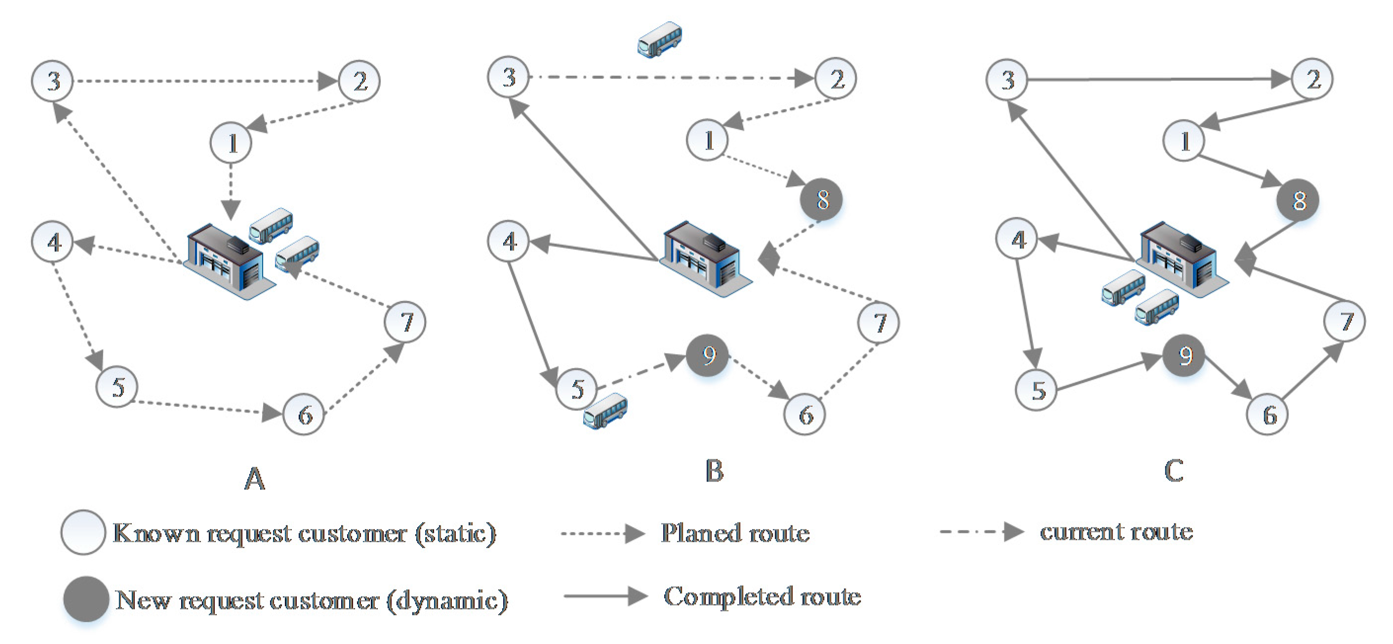
Figure 2.
Butterfly representation and solution decoding.

Figure 3.
Illustration of operators in the later perturbation.
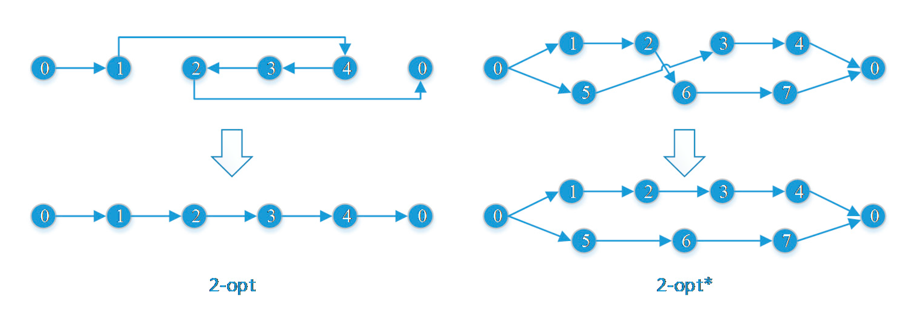
Figure 4.
Deviation from the known optimal solution.

Figure 5.
dispersion diagrams.

Table 1.
Comparison of the best Monarch Butterfly Optimization (MBO) results with the hitherto best-known solutions.
Table 1.
Comparison of the best Monarch Butterfly Optimization (MBO) results with the hitherto best-known solutions.
| MBO | BKS | Algorithm | RE (%) | TMBO (s) | |
|---|---|---|---|---|---|
| c50 | 570.61 | 551.95 | AAC-2OPT | 3.38 | 42.44 |
| c75 | 897.16 | 962.79 | GA | −6.82 | 83.01 |
| c100 | 915.27 | 961.10 | GA2007 | −4.77 | 80.80 |
| c100b | 819.60 | 800.93 | AAC-2OPT | 2.33 | 101.77 |
| c120 | 1070.18 | 1049.47 | AAC-2OPT | 1.97 | 122.56 |
| c150 | 1118.03 | 1318.22 | TS | −15.19 | 250.99 |
| c199 | 1394.74 | 1640.40 | DAPSO | −14.98 | 470.15 |
| f71 | 271.43 | 279.52 | DAPSO | −2.89 | 51.53 |
| f134 | 11759.06 | 13015.56 | AAC-2OPT | −9.77 | 205.78 |
| tai75a | 1748.71 | 1755.33 | AAC-2OPT | −0.38 | 81.75 |
| tai75b | 1371.90 | 1306.47 | AAC-2OPT | 5.01 | 90.42 |
| tai75c | 1464.37 | 1406.27 | TS | 4.13 | 77.41 |
| tai75d | 1419.00 | 1334.67 | AAC-2OPT | 6.32 | 83.13 |
| tai100a | 2185.49 | 2194.93 | AAC-2OPT | −0.43 | 113.82 |
| tai100b | 2057.80 | 2126.09 | AAC-2OPT | −3.21 | 108.28 |
| tai100c | 1463.42 | 1490.58 | VNS | −1.82 | 131.28 |
| tai100d | 1704.35 | 1834.60 | GA2007 | −7.10 | 119.77 |
| tai150a | 3560.28 | 2999.27 | AAC-2OPT | 18.70 | 336.75 |
| tai150b | 2966.19 | 2846.28 | AAC-2OPT | 4.21 | 333.55 |
| tai150c | 2528.04 | 2612.68 | GA2007 | −3.24 | 353.91 |
| tai150d | 2980.44 | 2950.61 | GA2007 | 1.01 | 292.68 |
| Average | 2107.91 | 2163.70 | −1.12 | 168.18 |
Table 2.
Comparison of the average MBO results with the hitherto best known solutions.
| MBO | BKS | Algorithm | RE (%) | TMBO (s) | |
|---|---|---|---|---|---|
| c50 | 590.73 | 570.89 | AAC-2OPT | 3.48 | 44.20 |
| c75 | 909.56 | 1013.45 | TS 2007 | −10.25 | 84.50 |
| c100 | 930.38 | 987.59 | GA 2007 | −5.79 | 82.43 |
| c100b | 839.93 | 841.44 | AAC-2OPT | −0.18 | 103.90 |
| c120 | 1112.58 | 1153.29 | AAC-2OPT | −3.53 | 126.08 |
| c150 | 1135.85 | 1386.93 | GA 2007 | −18.10 | 262.19 |
| c199 | 1414.40 | 1758.51 | AAC-2OPT | −19.57 | 492.80 |
| f71 | 277.00 | 306.33 | TS 2007 | −9.57 | 52.48 |
| f134 | 11853.29 | 15528.81 | AAC-2OPT | −23.87 | 215.09 |
| tai75a | 1799.15 | 1782.91 | AAC-2OPT | 0.91 | 83.63 |
| tai75b | 1385.45 | 1452.26 | AAC-2OPT | −4.60 | 93.61 |
| tai75c | 1483.41 | 1441.91 | AAC-2OPT | 2.88 | 81.09 |
| tai75d | 1435.62 | 1422.27 | AAC-2OPT | 0.94 | 86.42 |
| tai100a | 2212.08 | 2232.71 | AAC-2OPT | −0.92 | 116.53 |
| tai100b | 2105.15 | 2182.61 | AAC-2OPT | −3.55 | 111.98 |
| tai100c | 1474.32 | 1541.25 | GA 2014 | −4.04 | 137.05 |
| tai100d | 1722.88 | 1912.43 | AAC-2OPT | −10.78 | 123.70 |
| tai150a | 3539.61 | 3185.727 | AAC-2OPT | 8.78 | 375.45 |
| tai150b | 3038.38 | 2880.57 | AAC-2OPT | 5.48 | 365.32 |
| tai150c | 2641.62 | 2743.55 | AAC-2OPT | −3.72 | 377.15 |
| tai150d | 3047.30 | 3045.16 | GA 2007 | 0.07 | 322.49 |
| Average | 2140.41 | 2350.98 | −9.38 | 178.01 |
© 2017 by the authors. Licensee MDPI, Basel, Switzerland. This article is an open access article distributed under the terms and conditions of the Creative Commons Attribution (CC BY) license (http://creativecommons.org/licenses/by/4.0/).
Share and Cite
MDPI and ACS Style
Chen, S.; Chen, R.; Gao, J. A Monarch Butterfly Optimization for the Dynamic Vehicle Routing Problem. Algorithms 2017, 10, 107. https://doi.org/10.3390/a10030107
AMA Style
Chen S, Chen R, Gao J. A Monarch Butterfly Optimization for the Dynamic Vehicle Routing Problem. Algorithms. 2017; 10(3):107. https://doi.org/10.3390/a10030107
Chicago/Turabian StyleChen, Shifeng, Rong Chen, and Jian Gao. 2017. "A Monarch Butterfly Optimization for the Dynamic Vehicle Routing Problem" Algorithms 10, no. 3: 107. https://doi.org/10.3390/a10030107
Note that from the first issue of 2016, this journal uses article numbers instead of page numbers. See further details here.