Variable Selection Using Adaptive Band Clustering and Physarum Network


1
Chongqing Key Laboratory of Nonlinear Circuit and Intelligent Information Processing, Southwest University, Chongqing 400715, China
2
School of Electronic and Information Engineering, Southwest University, Chongqing 400715, China
*
Author to whom correspondence should be addressed.
Algorithms 2017, 10(3), 73; https://doi.org/10.3390/a10030073
Submission received: 19 April 2017
/
Revised: 21 June 2017
/
Accepted: 22 June 2017
/
Published: 27 June 2017
Abstract
:Variable selection is a key step for eliminating redundant information in spectroscopy. Among various variable selection methods, the physarum network (PN) is a newly-introduced and efficient one. However, the whole spectrum has to be equally divided into sub-spectral bands in PN. These division criteria limit the selecting ability and prediction performance. In this paper, we transform the spectrum division problem into a clustering problem and solve the problem by using an affinity propagation (AP) algorithm, an adaptive clustering method, to find the optimized number of sub-spectral bands and the number of wavelengths in each sub-spectral band. Experimental results show that combining AP and PN together can achieve similar prediction accuracy with much less wavelength than what PN alone can achieve.
1. Introduction
Spectroscopy has been widely used for quantitative analysis of complex samples in various fields, such as petrochemical, pharmaceutical, agricultural, food, and biological sectors. It is a non-invasive and efficient analytic technology that can be deployed in on-line analysis. To predict the concentration of one or more samples, a mathematical model has to be built to relate the spectrum (spectra) of the sample (samples) with the concentration. A common problem in spectroscopy is that the large number of spectral variables makes the prediction unreliable and complicates the prediction model. To reduce the dimensionality of the spectral date, projection methods [1], variable selection methods [2], or a combination of both [3,4,5] are used.
The projection methods, such as principle component analysis [6], partial least square (PLS) [7,8,9], discrete cosine transform [10], etc., change the high dimensional spectral data into low dimension space. The variable selection methods, such as the genetic algorithm (GA) [11,12,13], interval partial least square [2], etc. select a subset of variables to replace the original whole variable.
Considering the high correlation between adjacent spectral variables (wavelengths) due to the characteristics of the spectrograph, Chen et al. [14] transformed the variable selection problem into a path finding problem, i.e., the whole spectrum was divided into many sub-spectral bands. Each sub-spectral band was regarded as a node in a maze, every wavelength inside the sub-spectral band provided a route to its neighbor node; the shortest route (least correlation) was found by using a physarum network (PN) [15,16,17,18,19], and, thus, one wavelength from each sub-spectral band was selected, and the selected wavelengths had the least correlation. The PN is a mathematical model simulating the foraging process of plasmodium in a maze. This model has been proven to be able to compute the shortest path in the maze [15], and, thus, finds applications in many other fields, such as network design [16], sensor network [17], and supply chain network [19]. The PN can be used together with other variable selection methods to further reduce the dimensionality, i.e., it has been found that the PN-GA-PLS can achieve similar prediction performance with that of GA-PLS but uses much less wavelength.
The PN-GA-PLS algorithm is a sequential combination of PN, GA, and PLS. It uses PN to select one wavelength from each sub-spectral band, and then inputs these wavelengths into GA for further selection, during which the PLS acts as the evaluation function for guiding the selection. A comprehensive description of PN-GA-PLS can be found in [14]. In PN-GA-PLS, the whole spectrum is equally divided into M sub-spectral bands, each of which has P wavelengths. Many sets of M and P are tried, the final M and P are determined if they gave a minimum prediction error.
This dividing criteria in the PN-GA-PLS has one limitation in that the whole spectrum has to be equally divided, which only considers the characteristics of spectrometer. If the spectral features of the samples are also taken into account, the spectrum can be divided according to the correlation of spectral response at each wavelength, i.e., a sub-spectral band can include more wavelengths if the wavelengths within the band have high correlation with each other.
To solve the limitation of the PN-GA-PLS and make the spectrum division scheme automatic and adaptive to the spectral features, in this paper, we transformed the spectrum division problem into a clustering problem, and solved the problem by using an adaptive band clustering method or affinity propagation algorithm (AP). The main contribution of our work is three fold.
The first contribution is that we considered the spectral features of the probed samples for building a new spectrum division scheme.
The second contribution is that we regarded each sub-spectral band as a cluster of wavelengths and used AP to divide the whole spectrum into many sub-spectral bands according to the affinities of wavelengths.
The third contribution is that we applied AP before PN-GA-PLS to develop a new variable selection method.
The AP can automatically divide the whole spectrum into sub-spectral bands and each of the sub-spectral bands can be a different width. This dividing method considers both the characteristics of spectrometer and spectral features of the samples. By applying the AP before PN, the number of selected wavelengths can be further decreased without degrading the prediction performance. Compared with PN-GA-PLS and AP-GA-PLS, AP-PN-GA-PLS can achieve similar prediction precision with the least wavelengths. This reduction of wavelengths is vital in on-line, real-time analytical applications because less wavelength input may mean less computation load, less processing time, and simpler hardware design.
The rest of the paper is organized as follows: the theory of the AP algorithm and the step of applying AP-PN for variable selection are given of in Section 2; the three databases used for testing the algorithms and the settings of the algorithms are introduced in Section 3; the results and analysis are given in Section 4; the conclusion is provided in Section 5.
2. Theory
2.1. AP Algorithm
AP [20,21,22,23,24,25,26,27] is an unsupervised clustering algorithm. It clusters data points by identifying a set of centers (exemplars). Unlike other clustering algorithms that need an initial set of input exemplars, AP considers all data points as potential exemplars. Each data point is regarded as a node in a network, real-valued messages are transmitted along the edge of the network until a set of exemplars and clusters are found. Because of the unsupervised characteristics and good performance of AP, it has been used in many areas since its initial publishing [20], such as band selection [21] and data compression [24] in hyperspectral imaging, spatial clustering in geospatial data [22], statistical information extraction from high-dimensional data spaces [23], and identification of protein complexes from protein interaction graphs [26].
The input required by the AP is the real valued similarities between data point and point , which indicates how suitable the data point is for being the exemplar of data point . The input for each data point is called preference and is denoted as . The data point with a large preference has a higher chance of being selected as an exemplar. The values of the input preferences can influence the number of exemplars or clusters, i.e., the larger the is, the more exemplars the AP will give [20].
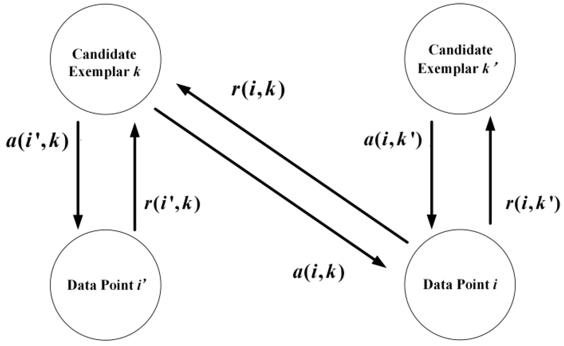
The messages passing through the edges are responsibility and availability. The responsibility reflects how well the point acts as an exemplar to the point . The availability reflects how well the point belongs to a class centered on point [20]. An illustration of message exchange in an AP network is given in Figure 1.
The and are calculated by using the formulas below
The and are calculated using different rules below
The responsibility and availability are updated constantly by using the rules below
where is the damping factor between 0 and 1 to avoid numerical oscillations, and are current and previous responsibility, respectively, and and are current and previous availability, respectively. The damping factor was set to a value between 0.5 and 0.9 following the suggestion in [21]. Different values of in the suggested range were tested. It was found that in this range has no effect on the final number of groups (see Section 3.1.2. Section 3.2.2. and Section 3.3.2. for details), so the is set as 0.9, which is the default value suggested in AP Algorithm software [20].
To begin with the update of and , all the availabilities are set to zero before the starting of Formula (1).
The exemplar of data point is the data point that makes the maximum.
The iteration of calculations can be stopped if a fixed step of iteration is reached or the exemplars stay constant for a fixed step of iteration.
2.2. Variable Selection Based on AP-PN
AP-PN is a sequential combination of AP and PN. It uses AP to automatically divide the whole spectrum into many sub-spectral bands that are not necessarily equal to each other and then selects one wavelength from each sub-spectral band by using PN. In AP-PN variable selection, a spectral response at a wavelength is regarded as a data point, a sub-spectral band is regarded as a cluster of data points. The input required by AP in this paper is the sample correlation coefficient [24] between wavelength and wavelength , which indicates to what extent the spectral information of the two wavelengths are correlated. It is calculated by using Formula (7)
where and represent the spectral response of the j-th sample at wavelength and , respectively, and are the average spectral response of all samples at wavelength and , respectively, and is the number of samples.
The preference is the input for controlling the number of clusters [20]. It is determined by maximizing the correlation function (shown in Formula (8)) or finding the point where the increasing trend of vanishes.
where is the total number of clusters, and represent the bands in the n-th cluster, is the number of wavelengths in the n-th cluster, and is the total number of wavelengths.
The steps of using AP-PN for variable selection are as follows:
- Calculate the similarity matrix according to the Formula (7);
- Set as a value between 0 to 1, staring from 0.00001 and updating by using ;
- Set , ;
- Calculate the responsibility information and availability information, and update them according to the Formulas(1)–(6);
- Determine the clusters, and go to step 2 until all are tried;
- Determine the according to Formula (8) and the corresponding clusters and exemplars;
- Bring the calculated clustering results into the PN for variable selection.
2.3. Complexity Analysis of AP-PN
The AP algorithm consists of two parts. The first part is to determine the value of . The time complexity of this part is , where is the number of bands selected in AP, is the number of wavelengths in each cluster, and it is not greater than 4, and is the number of total bands. In this paper, and are less than , so the time complexity of the first part of AP is . The second part of AP is to determine the clustering results. The time complexity of this part is . The space complexity of AP is . It is worth noting that the similarity matrix is calculated only once.
The time complexity of PN is , and the space complexity is .
3. Experiment
3.1. Corn Data Set
3.1.1. Data Set
This database is available at [28]. Three different Near Infrared (NIR) spectrometers were used to measure the corn samples. The whole spectrum was from 1100 to 2498 nm and the scanning resolution was 2 nm, namely, there were 700 wavelengths in total. There were 80 samples in the database. Each sample had four measured properties, i.e., water, oil, protein, and starch. The protein content was the property predicted in this paper. Numerical range of the protein content was from 7.6540 to 9.7110%. We used the hold-out method to select the training set and test set, i.e., we randomly selected the training and test sets. There were ten rounds of selection to generate the training set and test set. In each round, a training set and a test set were randomly produced. A training set consisted of 20 samples and a test set consisted of the remaining 60 samples. In addition, the performance of the model was assessed by the predicted root mean square error (RMSEP) and the correlation coefficient (R) between the predicted values and the real values in the test set. The RMSEP is defined in Formula (9)
where are the predicted values, are the measured values, and represents the number of the test sets.
3.1.2. Data Analysis
The AP-PN-GA-PLS, PLS, GA-PLS, PN-GA-PLS, and AP-GA-PLS were used for comparison. For PLS, the number of input wavelengths was the number of full-band variables.
For GA-PLS, the parameters of the GA-PLS model were set according to the literature [3], i.e., the population size was 30, the crossover probability was 50%, the mutation rate was 1%, and the iteration step was 100. The crossover is an operator used to generate child generation chromosome by exchanging the subsequences of the parent chromosomes. The crossover probability is the ratio indicating how many child generations are produced by crossover. The mutation is another operator to generate child generation chromosome by alerting one or more gene values in the parent chromosomes. The mutation rate is a ratio of the number of alerted genes to the whole number of genes. Before the GA-PLS was conducted, the ratio of the number of variables to the number of samples was checked by using the GAPLSOPT function in the PLS-Genetic Algorithm Toolbox provided by Leardi [3]. Averaging adjacent variables was done if the ratio did not pass the check.
For PN-GA-PLS, the parameters of the PN were set according to the literature [14], i.e., the total network traffic was 6, the number of iterations was 2000, the threshold of stop was 0.001, and the initial network continuity was 0.00001. The whole spectrum with W wavelengths was equally divided into M sub-spectral bands, each of which has P wavelengths (). If the sub-spectral band could not be equally divided (W/P is not an integer), each of the first to the (M-1)-th sub-spectral bands had P wavelengths, and the last sub-spectral band had wavelengths. Many sets of M and P were tried; M = 100 and P = 7 were determined because they gave the minimum RMSEP.
AP itself can give a representative (exemplar) for each sub-spectral band; it is not necessary to use PN after AP if every exemplar can be used directly to replace a corresponding sub-spectral band. Therefore, it is interesting to examine whether AP-GA-PLS can be used to replace AP-PN-GA-PLS. For the AP-GA-PLS, the settings were the same as those in AP-PN-GA-PLS. After the AP, the exemplars were used directly as the representative of the sub-spectral band, which were input to the GA-PLS.
For the AP-PN-GA-PLS, since we used the hold-out method to select the training set and the test set, the training set in each round was different and so too was the . In the first round, was set to 0.9, which is a default value suggested in the AP algorithm source code provided in [20], and the was then determined as 0.9996. We then fixed the value of and set to a value in the range of 0.5 to 0.9 to see whether the number of groups would change. It is shown in Table 1 that different values of produce the same number of groups (184). So we set to 0.9 in all the ten rounds. The other parameters of the PN network are the same as those in PN-GA-PLS.
3.2. Diesel Data Set
3.2.1. Data Set
The database is available at [29]. The dataset includes the near-infrared spectral data of the diesel samples and its corresponding property values. The whole spectrum was from 750 nm to 1550 nm, and the scanning resolution was 2 nm.
The property used in this research is the viscosity, whose numerical range is from 1.12 to 4.05. There were 395 data samples. We used the hold-out method to select the training set and test set. There were ten rounds for selecting the training set and test set. In each round, a training set and a test set were randomly produced. A training set consisted of 95 samples and a test set consisted of the remaining 300 samples.
3.2.2. Data Analysis
The AP-PN-GA-PLS, PLS, GA-PLS, PN-GA-PLS, and AP-GA-PLS were used for comparison. For the PLS, the number of input wavelengths was the number of the full-band variables.
For the GA-PLS, the parameters were set according to the literature [3]. The population size was 30, the crossover probability was 50%, the mutation rate was 1%, and the iteration step was 100. Before the GA-PLS was conducted, the ratio of the number of variables to the number of samples was checked by using the GAPLSOPT function in the PLS-Genetic Algorithm Toolbox provided by Leardi [3]. Averaging adjacent variables was done if the ratio did not pass the check.
For the PN-GA-PLS, the total network traffic was 6, the number of iterations was 2000, the threshold of filtering stop was 0.001, the initial network continuity was 0.00001, M = 120, and P = 3.
For the AP-PN-GA-PLS, was set to 0.9 in the first round, which is a default value suggested in the AP algorithm source code provided in [20], and the was then determined as 0.9953. We then fixed the value of and set to a value in the range of 0.5 to 0.9 to see whether the number of groups would change. It is shown in Table 2 that different value of produced the same number of groups (120), so we set to 0.9 in all the ten rounds. The other parameters of the PN network were the same as those in the PN-GA-PLS.
For the AP-GA-PLS, the settings were the same as those in the AP-PN-GA-PLS. After the AP, the exemplars were used directly as the representatives of the sub-spectral band, which were input into the GA-PLS.
3.3. Sweet Orange Leaves Data Set
3.3.1. Data Set
The data set contained chlorophyll with different concentrations of sweet orange leaves and was collected by the hyperspectral imaging system (HSI) used by Chongqing Metrology and Quality Inspection [14]. The HSI system consisted of a spectrometer and Charge-coupled Device (CCD) sensors, the spectral range was 400–1000 nm, scanning resolution was 0.74 nm–0.81 nm, and the channel was 761.
The is the reflection rate of sweet orange leaves, which can be represented as . Where is the image density, represents the density of white light, and denotes the density of dark light. After hyperspectral imaging, the mesophyll in the leaves was extracted from the veins. In order to extract chlorophyll from 0.02 g of mesophyll, we used 25 mL of 80% acetone, the concentration of the method described in [30].
One hundred thirty-three samples were included in this data set. We used the hold-out method to select the training set and the test set. There were ten rounds of selection to generate the training set and the test set. In each round, a training set and a test set were randomly produced. A training set consisted of 33 samples and a test set consisted of the remaining 100 samples.
3.3.2. Data Analysis
The AP-PN-GA-PLS, PLS, GA-PLS, PN-GA-PLS and AP-GA-PLS were used for comparison. For the PLS, the number of input wavelengths was the number of the full-band variables.
For the GA-PLS, the parameters were set according to the literature [3]. The population size was 30, the crossover probability was 50%, the mutation rate was 1%, and the iteration step was 100. Before the GA-PLS was conducted, the ratio of the number of variables to the number of samples was checked by using the GAPLSOPT function in the PLS-Genetic Algorithm Toolbox provided by Leardi [3]. Averaging adjacent variables was done if the ratio could not pass the check.
For the PN-GA-PLS, the total network traffic was 6, the number of iterations was 2000, the threshold of filtering stop was 0.001, the initial network continuity was 0.00001, M = 120, and P = 7.
For the AP-PN-GA-PLS, was set to 0.9 in the first selection, which is a default value suggested in the AP Algorithm source code provided in [20], and the was then determined as 0.99981. We then fixed the value of and set to a value in the range of 0.5 to 0.9 to see whether the number of groups would change. It is shown in Table 3 that different value of produce the same number of groups (234), so we set to 0.9 in all the ten rounds. The other parameters of the PN network were the same as those in the PN-GA-PLS.
For the AP-GA-PLS, the settings were the same as those in the AP-PN-GA-PLS. After the AP, the exemplars were used directly as the representatives of the sub-spectral band, which were input into the GA-PLS.
4. Results and Discussion
4.1. Corn Data Set
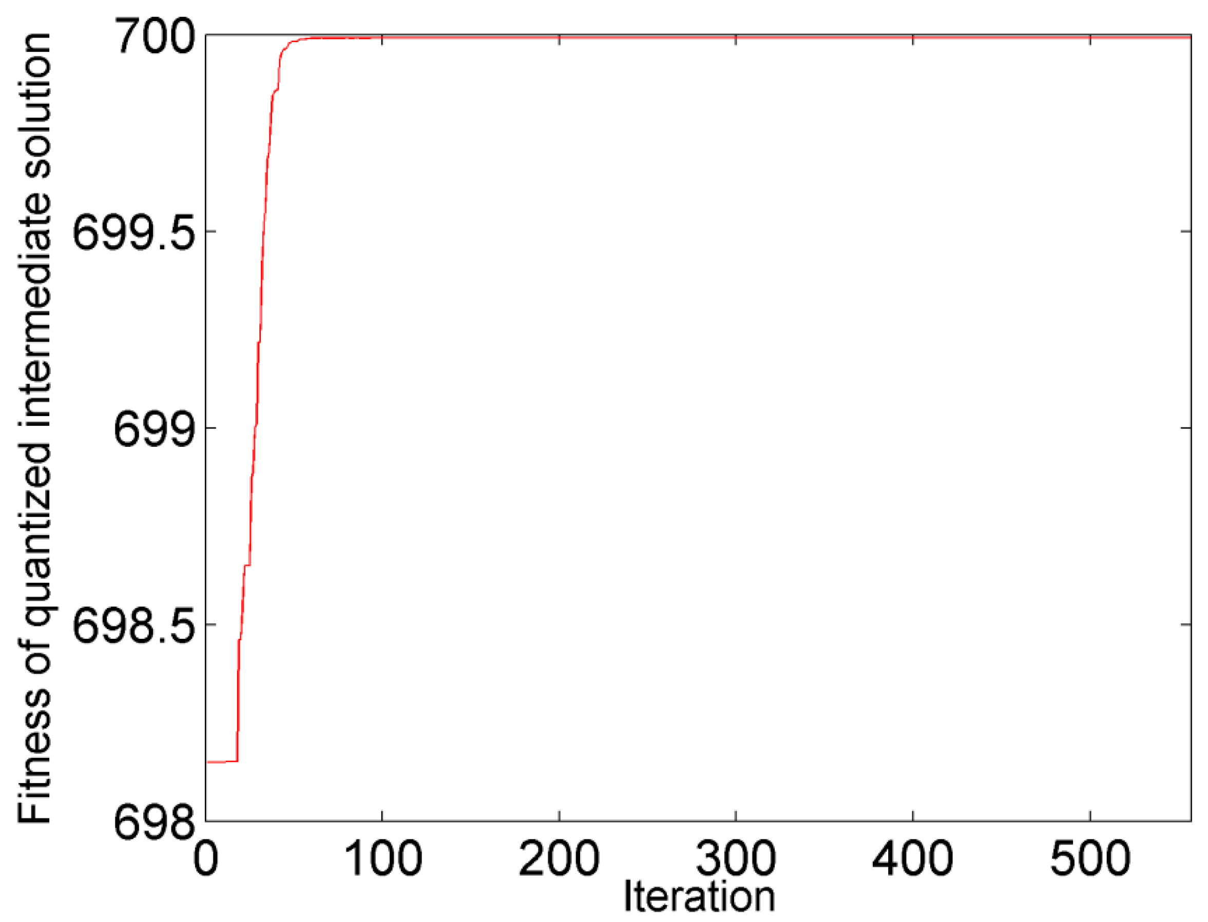
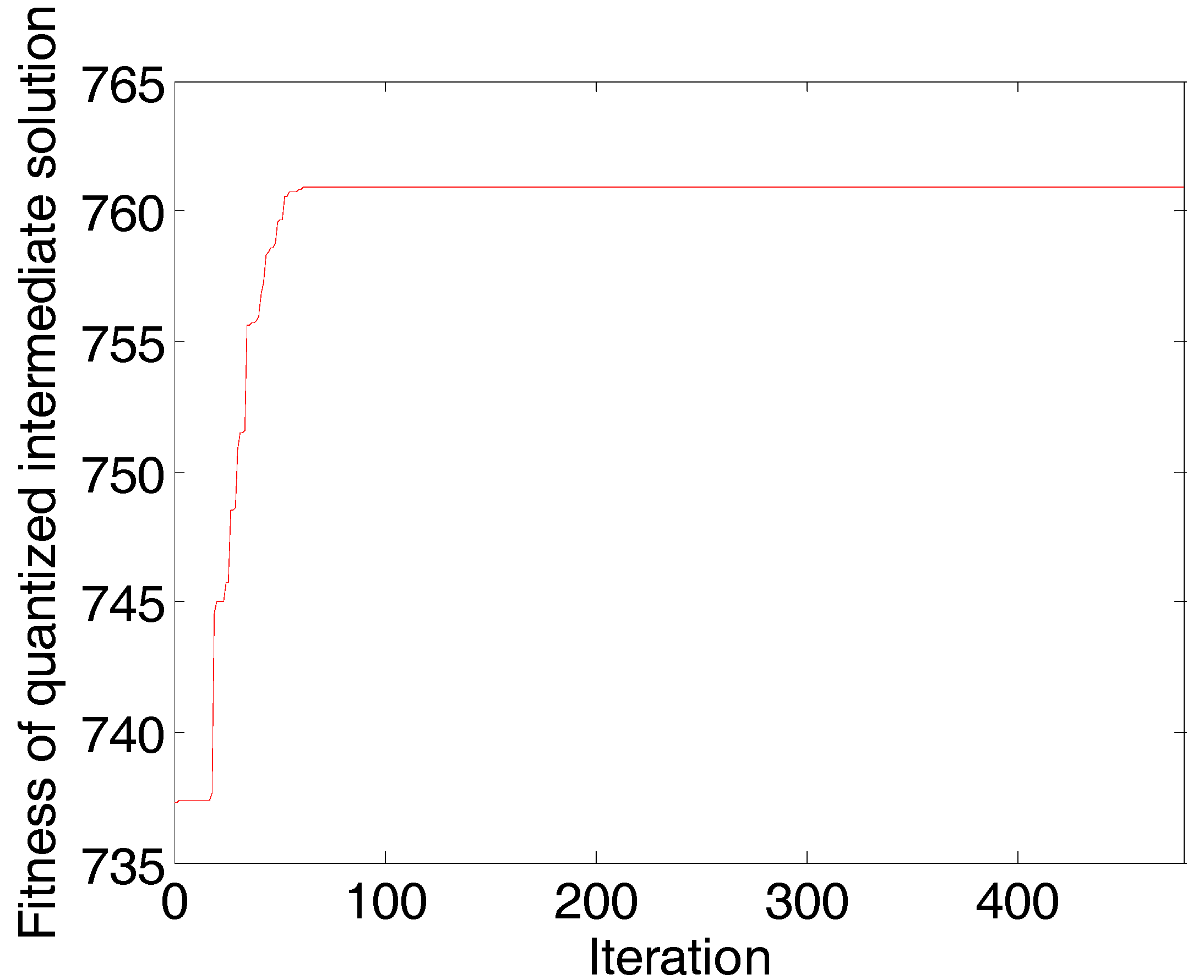
The convergence diagram of the AP algorithm run in the first round is shown in Figure 2. With the increase in the number of iterations, the fitness (net similarity) of quantized intermediate solutions gradually increases. When the number of iterations increases to 562, fitness no longer changes. The AP algorithm converges in the first round as well as in the rest of the rounds.
The convergence diagram of the PN algorithm run in the first round is shown in Figure 3. The represents the rate of change of the network continuity. The convergence condition of the PN algorithm is that all the rates of change of the network continuity are smaller than a threshold (0.001). Figure 3 shows the relationship of one of the rates of change of the network continuity and iterations. With an increase in the number of iterations, the gradually decreases. When the number of iterations increases to 10, all the are smaller than the threshold of stop. The PN algorithm converges in the first selection as well as in the rest of the rounds.
There were 184 wavelengths selected by the AP-PN in the first round, which are illustrated in Figure 4a. These 184 wavelengths were input into the GA-PLS. The times of each wavelength selected by GA-PLS are illustrated in Figure 4b. By using the 16 most selected wavelengths, the root mean square errors of cross-validation (, where represents the predicted value of the concentration of the i-th sample in the cross validation set, represents the measured value of the concentration of the i-th sample in the cross validation set, and is the number of cross validation sets) can reach the smallest value. These final 16 selected wavelengths found by using AP-PN-GA-PLS are illustrated in Figure 4c. The scatter plot of the predicted value vs. the measured value is given in Figure 4d. The curve that fits the data points best is also given in Figure 4d. The AP-PN-GA-PLS selected 16 wavelengths in the first round, which are shown in Figure 4c.
All five algorithms, i.e., PLS, GA-PLS, PN-GA-PLS, AP-GA-PLS, and AP-PN-GA-PLS, were tested on the ten rounds, and the average number of selected wavelengths, RMSEP, and Rare summarized in Table 4.
It is seen from Table 4 that the PN-GA-PLS can achieve similar prediction performance (RMSEP = 0.0597%) as that of GA-PLS (RMSEP = 0.0431%) but with fewer wavelengths (35 vs. 67). This result confirms the conclusion in the literature [14]. However, the number of wavelengths selected or the prediction performance of PN-GA-PLS in this research is larger or better than those of PN-GA-PLS in the literature [14], as are those of the GA-PLS. These differences in the number of selected wavelengths or prediction performance are due to the way in which training sets, test sets, and the sub-spectral bands were selected.
AP-PN-GA-PLS can achieve a similar prediction performance (RMSEP = 0.0397%) as that of PN-GA-PLS (RMSEP = 0.0597%) but with fewer wavelengths. The number of selected wavelengths of AP-PN-GA-PLS and PN-GA-PLS was 25 and 35, respectively. This may suggest that by using AP before PN, AP-PN-GA-PLS can further eliminate the redundant information in variables. Different from PN, AP optimized both the number of the sub-spectral bands and the number of the wavelengths within each sub-spectral band, therefore, AP-PN-GA-PLS can achieve similar prediction performance with less wavelength.
It is also shown in Table 4 that AP-GA-PLS can achieve RMSEP of 0.0643% with 39 wavelengths. This wavelength selection performance is comparable to that of PN-GA-PLS but is better than GA-PLS in terms of achieving similar RMSEP with less wavelength. This result suggests that the exemplars selected by AP can be input into GA-PLS directly, which can improve the wavelength selection performance.
However, AP-GA-PLS’s wavelength selection performance (39 wavelengths) is worse than that of AP-PN-GA-PLS (25 wavelengths). Every exemplar selected by the AP is a representative of each sub-spectral band, but it only represents the local information of the corresponding sub-spectral band. These exemplars do not consider the global information of the whole spectrum. They do not guarantee that they have the least correlation in a whole. This limitation of AP can be overcome by using PN afterwards. The PN selects one wavelength from each sub-spectral band to ensure that all the wavelengths in a whole have the least correlation. By combining the advantages of both AP and PN, the AP-PN-GA-PLS can thus achieve the best performance.
AP-PN-GA-PLS achieved very good prediction performance (R = 0.9970, RMSEP = 0.0397%) with the least number of wavelengths among PLS, GA-PLS, PN-GA-PLS, AP-GA-PLS, and AP-PN-GA-PLS, whose number of selected wavelengths were 700, 67, 35, 39, and 25, respectively.
There were 25 wavelengths selected by AP-PN-GA-PLS. The selected wavelengths 1778 nm and 1780 nm are similar to 1778 nm, which is the absorption wavelength of wheat gluten [31]. The selected wavelengths 2154 nm, 2156 nm, 2176 nm, and 2178 nm are within the range of 2100 nm–2200 nm, which are the absorption wavelengths of wheat gluten [31]. The selected wavelength 2220 nm is similar to 2230 nm, which is the local minimum absorption wavelength of wheat gluten [31].
4.2. Diesel Data Set
The convergence diagram of the AP algorithm is shown in Figure 5. With the increase of the number of iterations, the fitness (net similarity) of quantized intermediate solutions gradually increases. When the number of iterations increases to 386, and fitness no longer changes. The AP algorithm converges in the first round as well as in the rest of the rounds.
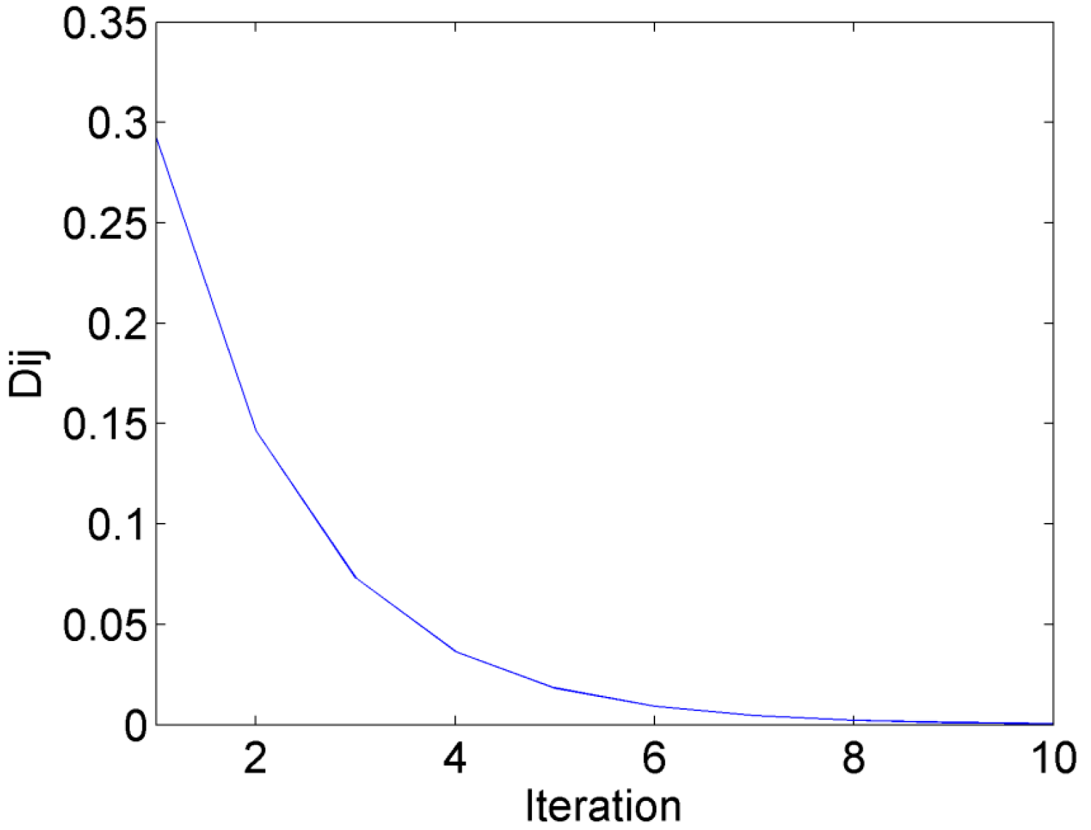
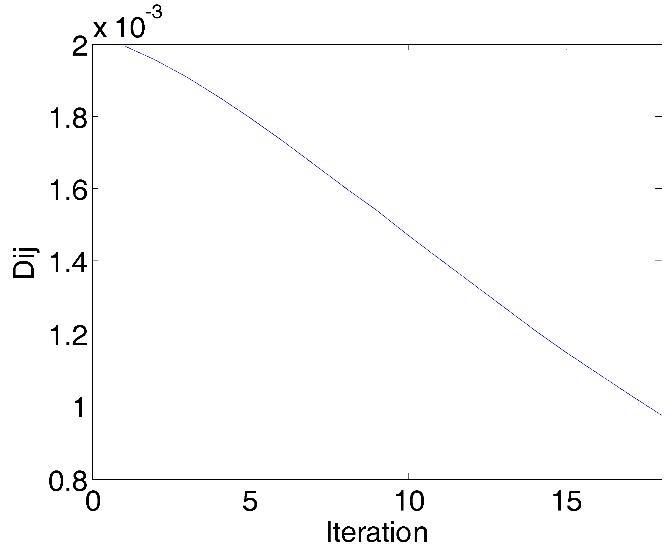
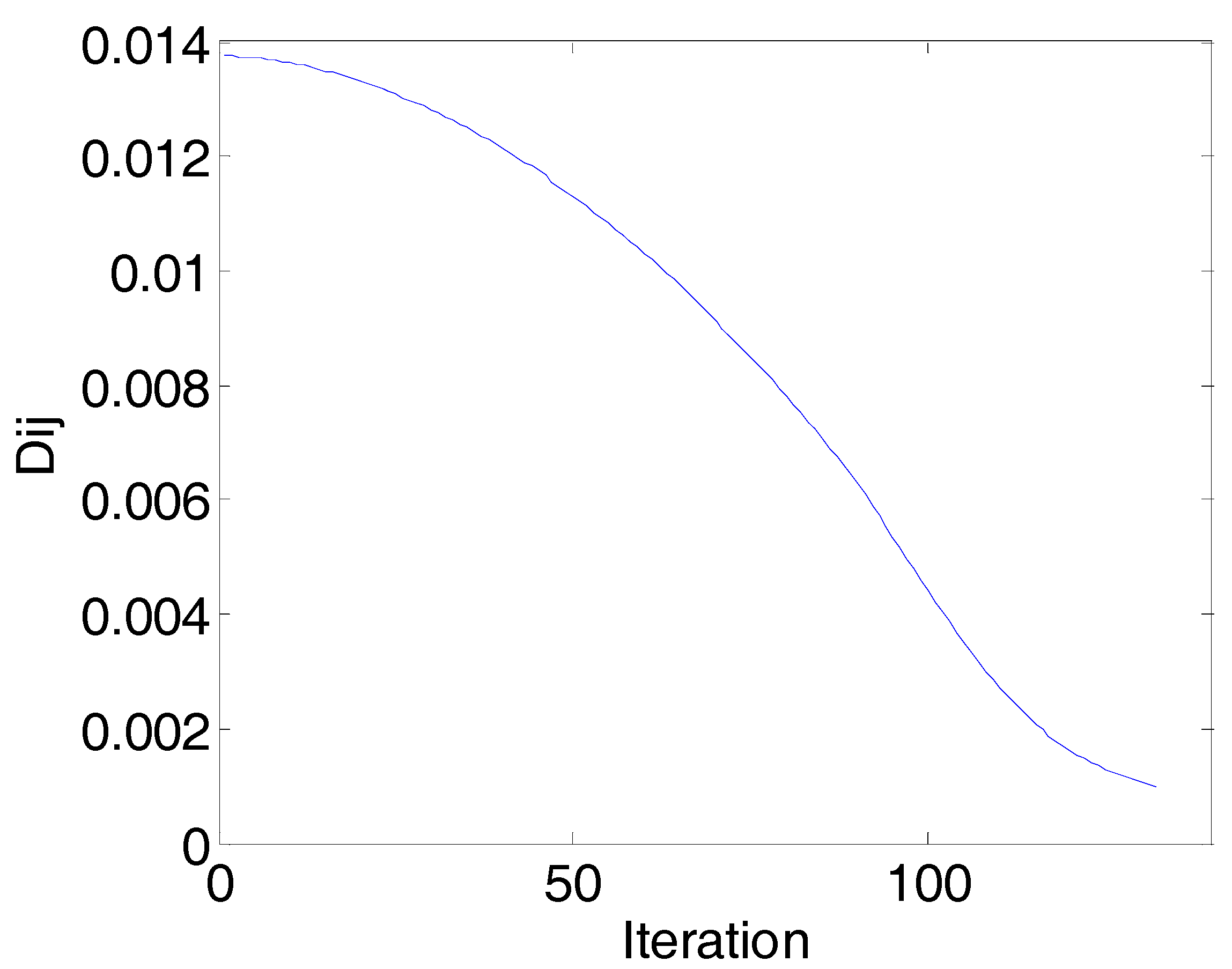
The convergence diagram of the PN algorithm is shown in Figure 6. The represents the rate of change of the network continuity. With the increase of the number of the iterations, the gradually decreases. When the number of iterations increases to 18, all the are smaller than the threshold of stop. The PN algorithm is converged.
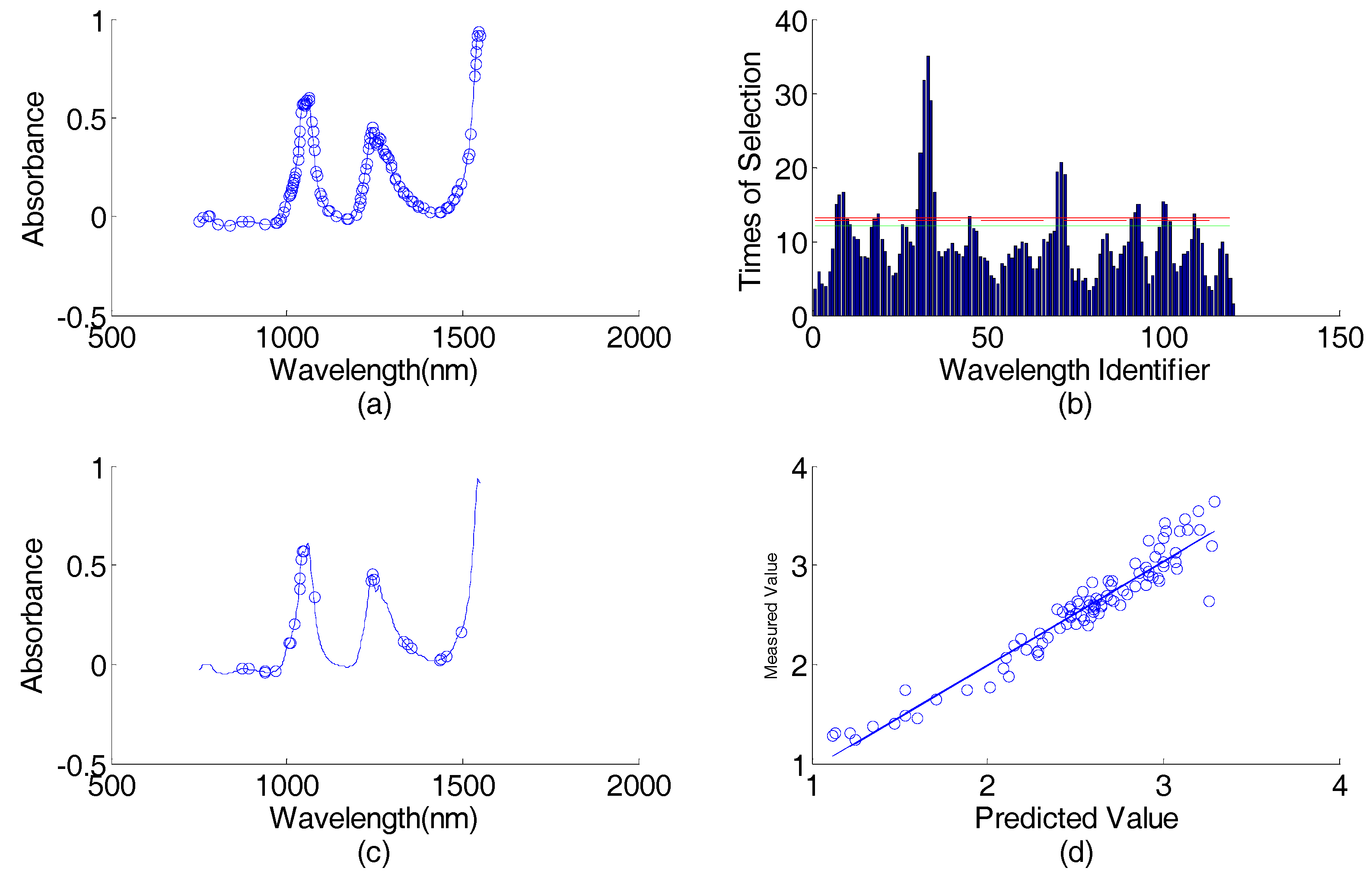
The number of wavelengths selected by using AP-PN in the first round was 120, which is illustrated in Figure 7a. These 120 wavelengths were input into GA-PLS. The times of each wavelength selected by GA-PLS are illustrated in Figure 7b. By using the 25 most selected wavelengths, the root mean square errors of cross-validation (RMSECV) can reach the smallest value. These final 25 selected wavelengths determined by using AP-PN-GA-PLS are illustrated in Figure 7c. The scatter plot of the predicted value vs. the measured value is given in Figure 7d. The curve that fits the data points best is also given in Figure 7d.
All five algorithms, i.e., PLS, GA-PLS, PN-GA-PLS, AP-GA-PLS, and AP-PN-GA-PLS, were tested in the ten rounds, and the average number of selected wavelength, RMSEP, and R are summarized in Table 5.
It is seen from Table 5 that AP-PN-GA-PLS can give the largest R (0.9744) and the smallest RMSEP (0.1167%) among PN-GA-PLS (R = 0.9727, RMSEP = 0.1404%), AP-GA-PLS (R = 0.9722, RMSEP = 0.1356%), and PLS (R = 0.9716, RMSEP = 0.1370%). It is also observed that the AP-PN-GA-PLS achieved good prediction performance with the least number of wavelengths among all methods. The number of selected wavelengths by AP-PN-GA-PLS was 26. The number of selected wavelengths by AP-GA-PLS, PN-GA-PLS, GA-PLS, and PLS were 66, 40, 142, and 401, respectively. The AP-PN-GA-PLS model may, thus, achieve the least complexity without degrading the prediction accuracy. The AP-GA-PLS can further reduce the redundant information in variables, compared with GA-PLS, but its wavelength selection performance (66 wavelengths selected, RMSEP = 0.1356%) is not as good as that of PN-GA-PLS (40 wavelengths selected, RMSEP = 0.1404%).
The AP-PN-GA-PLS selected 26 wavelengths. In general, the polycyclic aromatic hydrocarbon (PAHs) relates to the viscosity of diesel [32]. The final selected wavelengths of 942 nm and 1046 nm are similar to 934 nm and 1053 nm, respectively, which are the absorption wavelengths of methylene that relate to octane number. The selected wavelengths of 1422 nm and 1426 nm are the absorption wavelengths of the aromatic ring that relates to viscosity [32].
4.3. Sweet Orange Leaves Data Set
The convergence diagram of the AP algorithm in the first round is shown in Figure 8. With the increase of the number of iterations, the fitness (net similarity) of quantized intermediate solutions gradually increases. When the number of iterations increases to 486, fitness no longer changes. The AP algorithm converges in the first round as well as in the other rounds.
The convergence diagram of the PN algorithm in the first round is shown in Figure 9. The represents the rate of change of the network continuity. With the increase of the number of the iterations, the gradually decreases. When the number of iterations increases to 132, all the are smaller than the threshold of stop. The PN algorithm converges in the first round as well as in the other rounds.
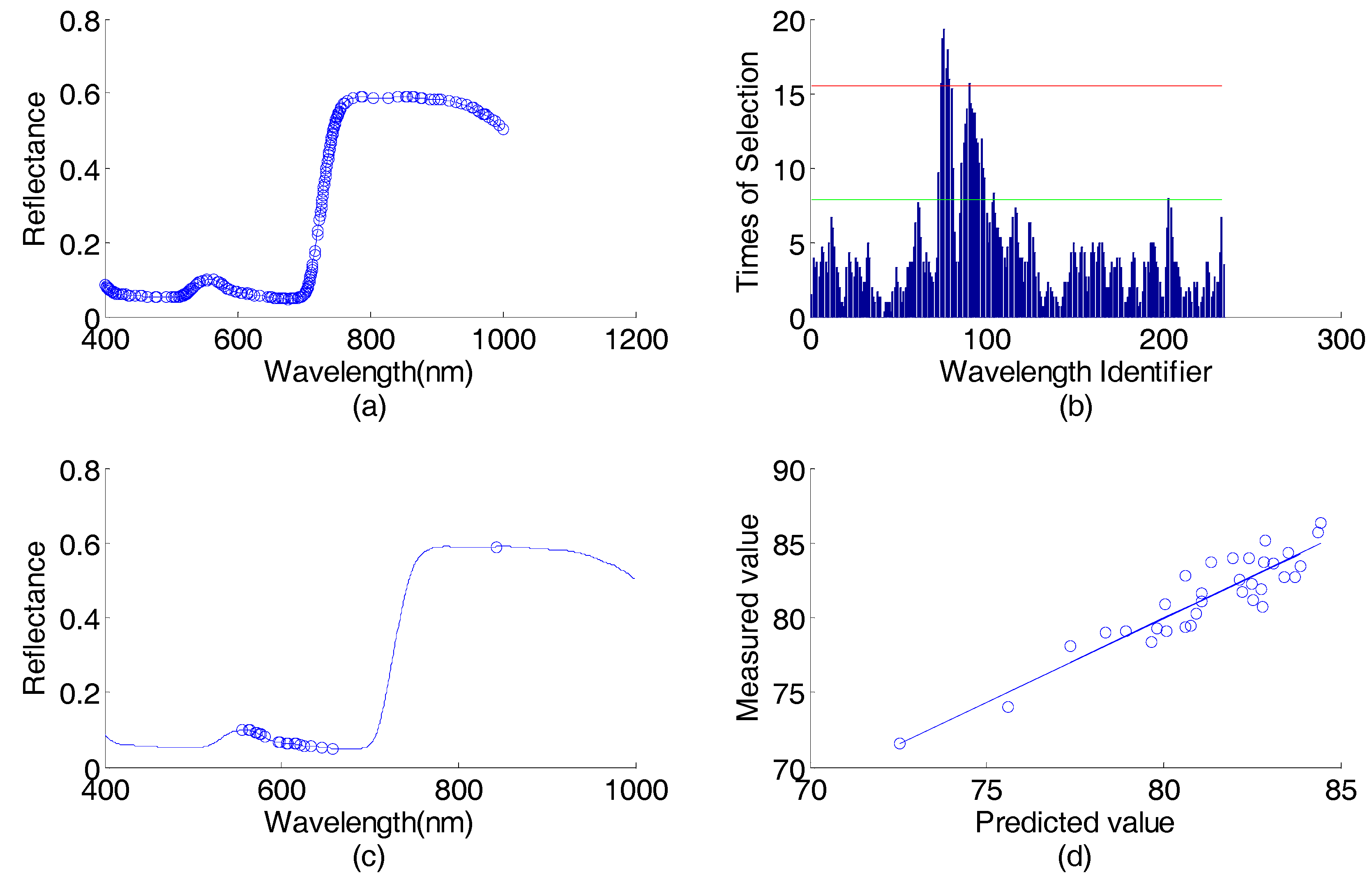
The number of wavelengths selected by using AP-PN was 234 in the first round, which is illustrated in Figure 10a. These 234 wavelengths were input into GA-PLS. The times of each wavelength selected by GA-PLS is illustrated in Figure 10b. By using the 25 most selected wavelengths, the RMSECV can reach smallest value. These final 25 wavelengths selected by using AP-PN-GA-PLS are illustrated in Figure 10c. The scatter plot of the predicted value vs. the measured value is given in Figure 10d. The curve that fits the data points best is also given in Figure 10d.
All five algorithms, i.e., PLS, GA-PLS, PN-GA-PLS, AP-GA-PLS, and AP-PN-GA-PLS, were tested in the ten rounds, and the average number of selected wavelength, RMSEP, and R are summarized in Table 6.
It is seen from Table 6 that the PN-GA-PLS can achieve similar prediction performance (RMSEP = 1.3206%) as that of GA-PLS (RMSEP = 1.4998%) but with fewer wavelengths (49 vs. 125). This result confirms the conclusion in the literature [14]. However, the number of wavelengths selected or the prediction performance of PN-GA-PLS in this research is larger or better than those of PN-GA-PLS in the literature [14], as are those of the GA-PLS. These differences in the number of selected wavelengths or prediction performance are due to the way in which training sets, test sets, and the sub-spectral bands were selected.
It is seen that AP-PN-GA-PLS can give the largest R (0.9220) and the smallest RMSEP (1.2436%) among PN-GA-PLS (R = 0.9110, RMSEP = 1.3206%), AP-GA-PLS (R = 0.9034, RMSEP = 1.4226%), GA-PLS (R = 0.9069, RMSEP = 1.4998%), and PLS (R = 0.9025, RMSEP = 1.4124%).
It is also observed that the AP-PN-GA-PLS achieved good prediction performance with the least number of wavelengths among all methods. The number of selected wavelengths by AP-PN-GA-PLS was 27. The numbers of selected wavelengths by AP-GA-PLS, PN-GA-PLS, GA-PLS, and PLS were 56, 49, 125, and 761, respectively. The AP-PN-GA-PLS model may, thus, achieve the least complexity without degrading the prediction accuracy.
The AP-PN-GA-PLS selected 27 wavelengths. The final selected wavelengths of 564 nm and 571 nm are similar to 568 nm. The selected wavelengths 581 nm is similar to 582 nm. The isotropic absorption point of chlorophyll is 568 nm and that of chlorophyll b is 582 nm [33]. The selected wavelength of 576 nm is the local maximum absorption wavelength of chlorophyll a [33]. The selected wavelength of 615 nm is similar to 614 nm, which is the local maximum absorption wavelength of chlorophyll a [33].
5. Conclusions
In spectroscopy, variable selection is important for the establishment of a prediction model. We proposed a method based on AP and PN for variable selection. The AP overcomes the PN’s limitation in dividing spectrum for building a network. Instead of dividing the spectrum equally, the AP can find optimized numbers of sub-spectral bands and numbers of wavelengths in each sub-spectral band.
The AP-PN can achieve higher prediction accuracy with fewer wavelengths than PN. It can also be combined with other variable selection methods, such as GA-PLS, to further eliminate the redundant information in variables and, thus, simplify the final prediction model and reduce the computation load.
The proposed algorithm has been tested on three databases. However, the amount of the samples in the databases is limited. To gain a large database is always a challenge. In future, the algorithm could be tested on simulated databases, in which artificial data with changeable parameters exist. By performing this simulation, more behaviors of the algorithm can be observed, which will help to improve the algorithm further.
Acknowledgments
We would like to acknowledge the support from the National Natural Science Foundation of China (Grant No. 61301297 and No. 61472330) and the Southwest University Doctoral Foundation (No. SWU115093).
Author Contributions
Tong Chen and Huanyu Chen conceived and designed the work. Huanyu Chen performed the data analysis. All authors wrote the paper.
Conflicts of Interest
The authors declare no conflicts of interest.
References
- Burges, C.J. Dimension reduction: Aguided tour. Found. Trends Mach. Learn. 2010, 2, 275–365. [Google Scholar] [CrossRef]
- Zou, X.; Zhao, J.; Povey, M.J.; Holmes, M.; Mao, H. Variables selection methods in near-infrared spectroscopy. Anal. Chim. Acta 2010, 667, 14–32. [Google Scholar]
- Leardi, R.; Gonzalez, A.L. Genetic algorithms applied to feature selection in PLS regression: How and when to use them. Chemom. Intell. Lab. Syst. 1998, 41, 195–207. [Google Scholar] [CrossRef]
- Ghasemi, J.; Niazi, A.; Leardi, R. Genetic-algorithm-based wavelength selection in multicomponent spectrophotometric determination by PLS: Application on copper and zinc mixture. Talanta 2003, 59, 311–317. [Google Scholar] [CrossRef]
- Durand, A.; Devos, O.; Ruckebusch, C.; Huvenne, J.P. Genetic algorithm optimization combined with partial least squares regression and mutual information variable selection procedures in near- infrared quantitative analysis of cotton–viscose textiles. Anal. Chim. Acta 2007, 595, 72–79. [Google Scholar] [CrossRef] [PubMed]
- Haaland, D.M.; Thomas, E.V. Partial least-squares methods for spectral analyses. 1. Relation to other quantitative calibration methods and the extraction of qualitative information. Anal. Chem. 1988, 60, 1193–1202. [Google Scholar]
- Geladi, P.; Kowalski, B.R. Partial least-squares regression: A tutorial. Anal. Chim. Acta 1986, 185, 1–17. [Google Scholar] [CrossRef]
- Mehmood, T.; Liland, K.H.; Snipen, L.; Sæbø, S. A review of variable selection methods in partial least squares regression. Chemom. Intell. Lab. Syst. 2012, 118, 62–69. [Google Scholar] [CrossRef]
- Wold, S.; Sjöström, M.; Eriksson, L. PLS-regression: A basic tool of chemometrics. Chemom. Intell. Lab. Syst. 2001, 58, 109–130. [Google Scholar] [CrossRef]
- Soh, C.S.; Raveendran, P.; Mukundan, R. Mathematical models for prediction of active substance content in pharmaceutical tablets and moisture in wheat. Chemom. Intell. Lab. Syst. 2008, 93, 63–69. [Google Scholar] [CrossRef]
- Roger, J.M.; Bellon-Maurel, V. Using genetic algorithms to select wavelengths in near-infrared spectra: Application to sugar content prediction in cherries. Appl. Spectrosc. 2000, 54, 1313–1320. [Google Scholar] [CrossRef]
- Leardi, R.; Seasholtz, M.B.; Pell, R.J. Variable selection for multivariate calibration using a genetic algorithm: Prediction of additive concentrations in polymer films from Fourier transform-infrared spectral data. Anal. Chim. Acta 2002, 461, 189–200. [Google Scholar] [CrossRef]
- Van, D.B.; Wienke, D.; Melssen, W.J.; Buydens, L.M.C. Optimal wavelength range selection by a genetic algorithm for discrimination purposes in spectroscopic infrared imaging. Appl. Spectrosc. 1997, 51, 1210–1217. [Google Scholar]
- Chen, T.; Zhao, X.C.; Zhou, H.; Liu, G.-Y. Selecting variables with the least correlation based on physarum network. Chemom. Intell. Lab. Syst. 2016, 153, 33–39. [Google Scholar] [CrossRef]
- Bonifaci, V.; Mehlhorn, K.; Varma, G. Physarum can compute shortest paths. J. Theor. Biol. 2012, 309, 121–133. [Google Scholar] [CrossRef] [PubMed]
- Liu, L.; Song, Y.; Zhang, H.; Ma, H.; Vasilakos, A.V. Physarum optimization: A biology-inspired algorithm for the steiner tree problem in networks. IEEE Trans. Comput. 2015, 64, 818–831. [Google Scholar]
- Song, Y.; Liu, L.; Ma, H.; Vasilakos, A.V. A biology-based algorithm to minimal exposure problem of wireless sensor networks. IEEE Trans. Netw. Serv. Manag. 2014, 11, 417–430. [Google Scholar] [CrossRef]
- Cheng, J.H.; Sun, D.W.; Wei, Q. Enhancing Visible and Near-Infrared Hyperspectral Imaging Prediction of TVB-N Level for Fish Fillet Freshness Evaluation by Filtering Optimal Variables. Food Anal. Methods 2016, 1–11. [Google Scholar] [CrossRef]
- Zhang, X.; Chan, F.T.S.; Adamatzky, A.; Mahadevan, S.; Yang, H.; Zhang, Z.; Deng, Y. An intelligent physarum solver for supply chain network design under profit maximization and oligopolistic competition. Int. J. Prod. Res. 2017, 55, 244–263. [Google Scholar] [CrossRef]
- Frey, B.J.; Dueck, D. Clustering by passing messages between data points. Science 2007, 315, 972–976. [Google Scholar] [CrossRef] [PubMed]
- Qian, Y.; Yao, F.; Jia, S. Band selection for hyperspectral imagery using affinity propagation. IET Comput. Vis. 2009, 3, 213–222. [Google Scholar] [CrossRef]
- Shi, X. Parallelizing Affinity Propagation Using Graphics Processing Units for Spatial Cluster Analysis over Big Geospatial Data. Adv. Geocomput. 2017, 355–369. [Google Scholar] [CrossRef]
- Clarke, R.; Ressom, H.W.; Wang, A.; Xuan, J.; Liu, M.C.; Gehan, E.A.; Wang, Y. The properties of high-dimensional data spaces: Implications for exploring gene and protein expression data. Nat. Rev. Cancer 2008, 8, 37–49. [Google Scholar] [CrossRef] [PubMed]
- Chen, S.X.; Can, H.; Qu, L.Y. Hyperspectral Image Compression Based on Adaptive Band Clustering PCA. Sci. Technol. Eng. 2015, 15, 86–91. [Google Scholar]
- Dueck, D.; Frey, B.J. Non-metric affinity propagation for unsupervised image categorization. In Proceedings of the IEEE 11th International Conferenceon Computer Vision (ICCV), Rio de Janeiro, Brazil, 14–21 October 2007. [Google Scholar]
- Vlasblom, J.; Wodak, S.J. Markov clustering versus affinity propagation for the partitioning of protein interaction graphs. BMC Bioinform. 2009, 10, 99. [Google Scholar] [CrossRef] [PubMed]
- Givoni, I.E.; Frey, B.J. A binary variable model for affinity propagation. Neural Comput. 2009, 21, 1589–1600. [Google Scholar] [CrossRef] [PubMed]
- NIR of Corn Samples for Standardization Benchmarking. Available online: http://www.eigenvector.com/data/Corn/ (accessed on 26 June 2017).
- Near Infrared Spectra of Diesel Fuels. Available online: http://www.eigenvector.com/data/SWRI/index.html (accessed on 26 June 2017).
- Lichtenthaler, H.K. Chlorophylls and carotenoids: pigments of photosynthetic biomembranes. Methods Enzymol. 1987, 148, 350–382. [Google Scholar]
- Burns, D.A.; Ciurczak, E.W. Handbook of Near-Infrared Analysis, 3rd ed.; CRC Press: New York, NY, USA, 2016. [Google Scholar]
- Shen, Y.J. Effects of Polycyclic Aromatic Hydrocarbons on Diesel Particulate Matter Emission. Pet. Prod. Appl. Res. 2006, 3, 85–87. [Google Scholar]
- Zscheile, F.P.; Comar, C.L. Influence of preparative procedure on the purity of chlorophyll components as shown by absorption spectra. Bot. Gaz. 1941, 102, 463–481. [Google Scholar] [CrossRef]
Figure 1.
Two messages, responsibility (, , and ), and availability (, , and ), are passing in an affinity propagation network. The responsibility and reflect how well the point acts as an exemplar to the point and , respectively. The availability and reflect how well the point and belong to a class centered on point . The responsibility reflects how well the point acts as an exemplar to the point . The availability reflects how well the point belongs to a class centered on point .

Figure 2.
The convergence diagram of the affinity propagation (AP) algorithm (corn data) in the first round: Iterations vs. Fitness (net similarity) of quantized intermediate solutions. When the iteration is 562, the network is converged.
Figure 2.
The convergence diagram of the affinity propagation (AP) algorithm (corn data) in the first round: Iterations vs. Fitness (net similarity) of quantized intermediate solutions. When the iteration is 562, the network is converged.

Figure 3.
The convergence diagram of the physarum network (PN) algorithm (corn data) in the first round: Iterations vs. (Dij is the rate of change of the network continuity). When the iteration is 10, all the Dij are smaller than the threshold of stop, and the network converges.
Figure 3.
The convergence diagram of the physarum network (PN) algorithm (corn data) in the first round: Iterations vs. (Dij is the rate of change of the network continuity). When the iteration is 10, all the Dij are smaller than the threshold of stop, and the network converges.

Figure 4.
Corn data (predicting protein content) wavelength selection result by using AP-PN-GA-PLS in the first round: (a) spectral responses vs. wavelengths, the 184 wavelengths selected by AP-PN are marked with circles; (b) times of selection (by GA-PLS) vs. wavelength identifier (1–184), the wavelengths above the lower line were selected; (c) spectral response vs. wavelengths, the 16 wavelengths selected by AP-PN-GA-PLS are marked with circles; (d) scatter plot of predicted values vs. the measured values. PLS = partial least square; GA = genetic algorithm.
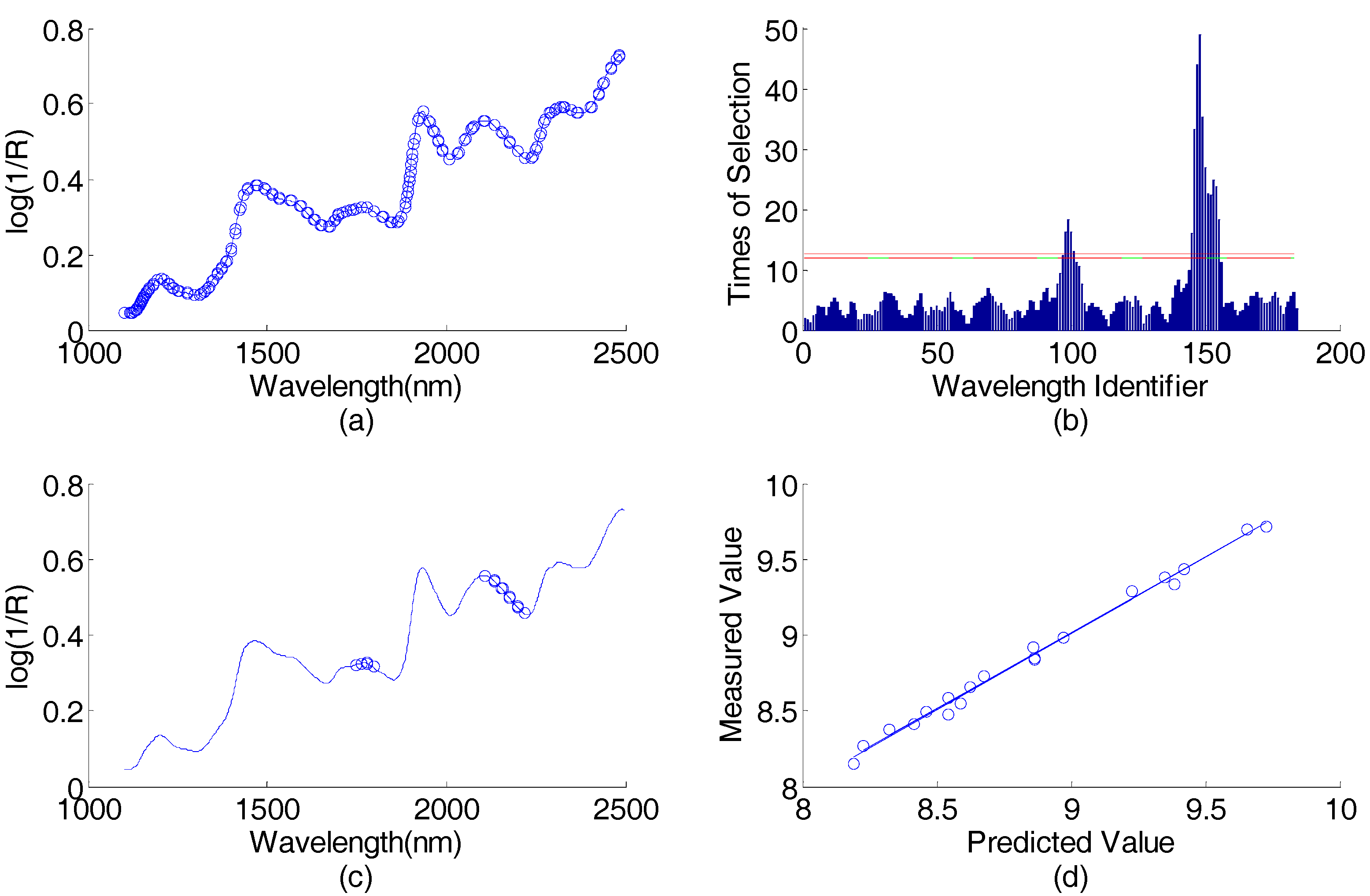
Figure 5.
The convergence diagram of the AP algorithm (diesel data): Iterations vs. Fitness (net similarity) of quantized intermediate solution in the first round. When the iteration is 386, the network is converged.
Figure 5.
The convergence diagram of the AP algorithm (diesel data): Iterations vs. Fitness (net similarity) of quantized intermediate solution in the first round. When the iteration is 386, the network is converged.
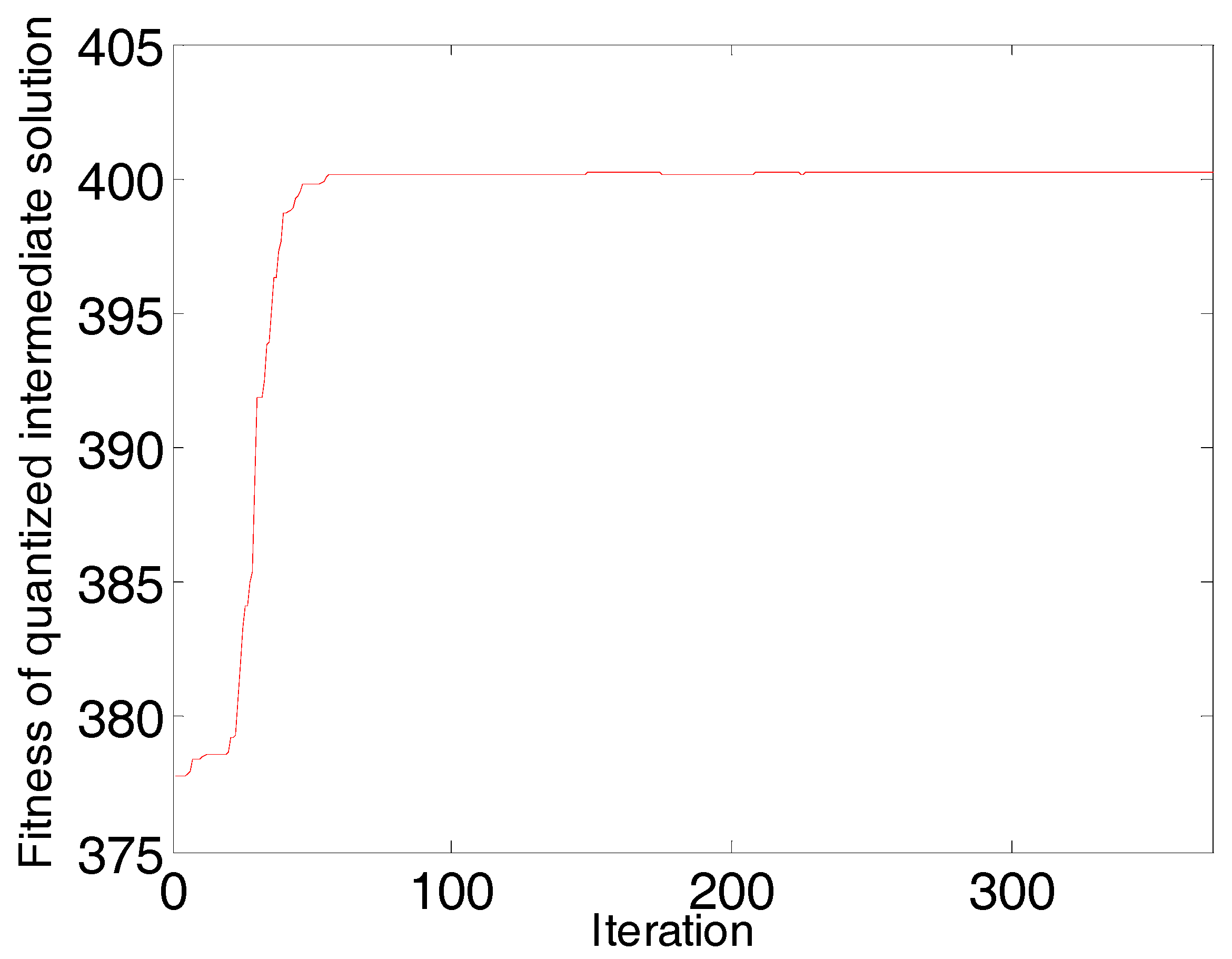
Figure 6.
The convergence diagram of the PN algorithm (corn data): Iterations vs. (Dij is the rate of change of the network continuity). When the iteration is 18, all the Dij are smaller than the threshold of stop, and the network is converged.
Figure 6.
The convergence diagram of the PN algorithm (corn data): Iterations vs. (Dij is the rate of change of the network continuity). When the iteration is 18, all the Dij are smaller than the threshold of stop, and the network is converged.

Figure 7.
Diesel data (predicting viscosity content) wavelength selection result in the first round: (a) spectral responses vs. wavelengths, the 120 wavelengths selected by AP-PN are marked with circles; (b) times of selection (by GA-PLS) vs. wavelength identifier (1–120); (c) spectral response vs. wavelengths, the 25 wavelengths selected by AP-PN-GA-PLS are marked with circles; (d) scatter plot of predicted values vs. the measured values.

Figure 8.
The convergence diagram of the AP algorithm (sweet orange leaves data) in the first round: Iterations vs. Fitness (net similarity) of quantized intermediate solutions. When the iteration is 486, the network is converged.
Figure 8.
The convergence diagram of the AP algorithm (sweet orange leaves data) in the first round: Iterations vs. Fitness (net similarity) of quantized intermediate solutions. When the iteration is 486, the network is converged.

Figure 9.
The convergence diagram of the PN algorithm (corn data) in the first round: Iterations vs. (Dij is the rate of change of the network continuity). When the iteration is 132, all the Dij are smaller than the threshold of stop, and the network is converged.
Figure 9.
The convergence diagram of the PN algorithm (corn data) in the first round: Iterations vs. (Dij is the rate of change of the network continuity). When the iteration is 132, all the Dij are smaller than the threshold of stop, and the network is converged.

Figure 10.
Sweet orange leaves data (predicting viscosity content) wavelength selection results in the first round: (a) spectral responses vs. wavelengths, the 234 wavelengths selected by AP-PN are marked with circles; (b) times of selection (by GA-PLS) vs. wavelength identifier (1–234); (c) spectral response vs. wavelengths, the 25 wavelengths selected by AP-PN-GA-PLS are marked with circles; (d) scatter plot of predicted values vs. the measured values.

Table 1.
The relationship between and the number of groups (corn data).
| 0.5 | 0.6 | 0.7 | 0.8 | 0.9 | |
| Number of groups | 184 | 184 | 184 | 184 | 184 |
Table 2.
The relationship between and the number of groups (diesel data).
| 0.5 | 0.6 | 0.7 | 0.8 | 0.9 | |
| Number of groups | 120 | 120 | 120 | 120 | 120 |
Table 3.
The relationship between and the number of groups (orange leaves data).
| 0.5 | 0.6 | 0.7 | 0.8 | 0.9 | |
| Number of groups | 234 | 234 | 234 | 234 | 234 |
Table 4.
The average values of the number of selected wavelengths, correlation coefficient (R), and predicted root mean square error (RMSEP) using PLS, GA-PLS, PN-GA-PLS, AP-GA-PLS, and AP-PN-GA-PLS (corn data).
Table 4.
The average values of the number of selected wavelengths, correlation coefficient (R), and predicted root mean square error (RMSEP) using PLS, GA-PLS, PN-GA-PLS, AP-GA-PLS, and AP-PN-GA-PLS (corn data).
| Method | Number of Input Wavelengths | Number of Selected Wavelengths | R | RMSEP(%) |
|---|---|---|---|---|
| PLS | 700 | 700 | 0.9832 | 0.0902 |
| GA-PLS | 700 | 67 | 0.9989 | 0.0431 |
| PN-GA-PLS | 700 | 35 | 0.9960 | 0.0597 |
| AP-GA-PLS | 700 | 39 | 0.9941 | 0.0643 |
| AP-PN-GA-PLS | 700 | 25 | 0.9970 | 0.0397 |
Table 5.
The average values of the number of selected wavelengths, R, and RMSEP using PLS, GA-PLS, PN-GA-PLS, AP-GA-PLS, and AP-PN-GA-PLS (diesel data).
Table 5.
The average values of the number of selected wavelengths, R, and RMSEP using PLS, GA-PLS, PN-GA-PLS, AP-GA-PLS, and AP-PN-GA-PLS (diesel data).
| Method | Number of Input Wavelengths | Number of Selected Wavelengths | R | RMSEP(%) |
|---|---|---|---|---|
| PLS | 401 | 401 | 0.9716 | 0.1370 |
| GA-PLS | 401 | 142 | 0.9739 | 0.1203 |
| PN-GA-PLS | 401 | 40 | 0.9727 | 0.1404 |
| AP-GA-PLS | 401 | 66 | 0.9722 | 0.1356 |
| AP-PN-GA-PLS | 401 | 26 | 0.9744 | 0.1167 |
Table 6.
The average values of the number of selected wavelengths, R, and RMSEP using PLS, GA-PLS, PN-GA-PLS, AP-GA-PLS, and AP-PN-GA-PLS (orange leaves data).
Table 6.
The average values of the number of selected wavelengths, R, and RMSEP using PLS, GA-PLS, PN-GA-PLS, AP-GA-PLS, and AP-PN-GA-PLS (orange leaves data).
| Method | Number of Input Wavelengths | Number of Selected Wavelengths | R | RMSEP (%) |
|---|---|---|---|---|
| PLS | 761 | 761 | 0.9025 | 1.4124 |
| GA-PLS | 761 | 125 | 0.9069 | 1.4998 |
| PN-GA-PLS | 761 | 49 | 0.9110 | 1.3206 |
| AP-GA-PLS | 761 | 56 | 0.9034 | 1.4226 |
| AP-PN-GA-PLS | 761 | 27 | 0.9220 | 1.2436 |
© 2017 by the authors. Licensee MDPI, Basel, Switzerland. This article is an open access article distributed under the terms and conditions of the Creative Commons Attribution (CC BY) license (http://creativecommons.org/licenses/by/4.0/).
Share and Cite
MDPI and ACS Style
Chen, H.; Chen, T.; Zhang, Z.; Liu, G. Variable Selection Using Adaptive Band Clustering and Physarum Network. Algorithms 2017, 10, 73. https://doi.org/10.3390/a10030073
AMA Style
Chen H, Chen T, Zhang Z, Liu G. Variable Selection Using Adaptive Band Clustering and Physarum Network. Algorithms. 2017; 10(3):73. https://doi.org/10.3390/a10030073
Chicago/Turabian StyleChen, Huanyu, Tong Chen, Zhihao Zhang, and Guangyuan Liu. 2017. "Variable Selection Using Adaptive Band Clustering and Physarum Network" Algorithms 10, no. 3: 73. https://doi.org/10.3390/a10030073
Note that from the first issue of 2016, this journal uses article numbers instead of page numbers. See further details here.