A Genetic Algorithm Using Triplet Nucleotide Encoding and DNA Reproduction Operations for Unconstrained Optimization Problems


1
School of Management Science and Engineering, Shandong Normal University, Jinan 250014, China
2
Department of Computer Science, University of Texas at San Antonio, San Antonio, TX 78249, USA
*
Author to whom correspondence should be addressed.
Algorithms 2017, 10(3), 76; https://doi.org/10.3390/a10030076
Submission received: 31 May 2017
/
Revised: 19 June 2017
/
Accepted: 19 June 2017
/
Published: 30 June 2017
Abstract
:As one of the evolutionary heuristics methods, genetic algorithms (GAs) have shown a promising ability to solve complex optimization problems. However, existing GAs still have difficulties in finding the global optimum and avoiding premature convergence. To further improve the search efficiency and convergence rate of evolution algorithms, inspired by the mechanism of biological DNA genetic information and evolution, we present a new genetic algorithm, called GA-TNE+DRO, which uses a novel triplet nucleotide coding scheme to encode potential solutions and a set of new genetic operators to search for globally optimal solutions. The coding scheme represents potential solutions as a sequence of triplet nucleotides and the DNA reproduction operations mimic the DNA reproduction process more vividly than existing DNA-GAs. We compared our algorithm with several existing GA and DNA-based GA algorithms using a benchmark of eight unconstrained optimization functions. Our experimental results show that the proposed algorithm can converge to solutions much closer to the global optimal solutions in a much lower number of iterations than the existing algorithms. A complexity analysis also shows that our algorithm is computationally more efficient than the existing algorithms.
1. Introduction
Optimization problems arise in many real-world applications and various types of intelligent evolutionary optimization methods, such as the Genetic Algorithm (GA) [1], the Particle Swarm Optimization (PSO) [2], the Differential Evolution (DE) [3], and the artificial bee colony (ABC) [4], have been proposed in the literature over the last few decades. The PSO algorithm is based on a simulation of social behavior and has been applied in various optimization problems [5]. The DE algorithm employs the difference of parameter vectors to explore the objective function [6]. The Genetic Algorithm, proposed by Holland in 1975, is an algorithmic model for solving optimization problems and is inspired by genetic evolution. The conventional GA encodes a possible solution in the solution space as a string of binary bits which is treated as (a chromosome of) an individual. It explores the search space for optimal solutions by generating new individuals from an individual in the current population, using a set of operations that mimic genetic mutation in natural evolution. This approach has shown some success in solving complex optimization problems. However, the traditional GA has several drawbacks. It often suffers from a premature convergence to a local optimum when searching in a local area if there is a rapid decrease in population diversity. In addition, the binary bit string encoding usually results in a very long code and therefore, significantly reduces the computational efficiency. Many researchers believe that a promising solution to these problems may lie in the adaptation of more sophisticated natural models that can be incorporated into the framework of the GA algorithms. Hybrid optimization algorithms have recently been proposed to overcome the existing drawbacks of GA [7]. Pelusi et al. proposed a revised Gravitational Search Algorithm (GSA) [8] powered by evolutionary methods and obtained good results. Garg proposed a hybrid technique known as PSO-GA [9] for solving the constrained optimization problems.
On the other hand, mimicking the genetic mechanisms of biological DNA in computation has gained increasing interest in the computer science research community [10]. This was inspired by the fact that, as the major genetic material in life, DNA encodes and processes an enormous amount of genetic information. DNA computing, proposed by Adleman [11] in 1994, may potentially provide a promising method for solving complex optimization problems because its parallel computing may efficiently search through a large space for potential solutions [12]. However, using DNA as computing hardware [13] still faces many challenges. For example, current solutions require biological experiments which are expensive and time-consuming.
Integrating genetic algorithms with DNA computing can provide a promising alternative for solving complex optimization problems. Extending GA to use DNA encoding and corresponding genetic operations is a natural extension to the GA and DNA-computing techniques, which both aim to solve complex computational problems by mimicking a process in nature. Recent developments in the understanding of biological DNA has provided a solid ground for research. For example, a PID controller [14] and many other applications [15] have been designed using DNA computing. The DNA sequence is arguably more suitable for encoding individuals in a genetic algorithm than simple binary bit strings for solving optimization problems. The current research in this area is focused on developing better DNA encoding [16,17].
A DNA genetic algorithm (DNA-GA) was initially proposed by Ding [18] and a modified DNA genetic algorithm (MDNA-GA) was subsequently introduced by Zhang and Wang [19]. In these algorithms, DNA encoding and two DNA-based operators, the choose crossover and frame-shift mutation, were used. These methods have been shown to be effective in improving the search for global solutions. A method was also used in these algorithms to break from a local optimum, so that a larger portion of the search space can be explored to accelerate the convergence towards the global optimum. Chen and Wang presented a DNA-based hybrid genetic algorithm (DNA-HGA) for nonlinear optimization problems [20], in which potential solutions are encoded as nucleotide bases and genetic operators use the complementary properties of nucleotide bases to efficiently locate feasible solutions. Zhang et al. proposed an adaptive RNA genetic algorithm (ARNA-GA) [21] which used RNA encoding to represent potential solutions and new RNA-based genetic operators to improve the global search. Noticeably, ARNA-GA deploys an adaptive genetic strategy that dynamically chooses between a crossover operation and mutation operation based on a dissimilarity coefficient. Zang et al. presented a DNA genetic algorithm that is modeled after a biological membrane structure [22].
DNA-based GA methods have been successfully applied to solve many difficult optimization problems. Sun et al. employed RNA-GA in a double inverted pendulum system and showed an improved performance [23]. Zang et al. have adapted DNA-GA to solve several pattern recognition problems, including clustering analysis, classification, and multi-object optimization [24,25,26].
Although much progress has been made to improve DNA-based genetic algorithms, further study is still needed to improve the speed at which the search converges to the global optimum and to prevent the algorithm from been locked to a local optimum. The focus is to find an efficient coding scheme, better genetic operations, and better convergence control.
In this paper, we present a new GA, called GA-TNE+DRO, which uses a novel triplet nucleotide coding scheme to encode individuals of GA and provides a set of novel genetic operators that mimic DNA molecule genetic operations. Specifically, we make the following contributions in this paper.
- We define a new DNA coding scheme which encodes the potential solution problem space using triplet nucleotides that represent amino acids.
- We define a set of evolutional operations that create new individuals in the problem space by mimicking the DNA reproduction process at an amino acid level.
- We present a genetic algorithm that uses triplet nucleotide encoding (TNE) and a DNA reproduction operator (DRO), hence the name GA-TNE+DRO.
- We perform experiments to evaluate the performance of the algorithm using a benchmark of eight unconstrained optimization problems and compare it with state-of-the-art algorithms including conventional GA [1], PSO [2], and DE [3]. Our experimental results show that our algorithm can converge to solutions much closer to the global optimal solutions in a much lower number of iterations than the existing algorithms.
The remainder of this paper is organized as follows. Section 2 presents the triplet nucleotide code scheme. Section 3 presents a set of genetic operations that are based on DNA triplet nucleotide encoding. Section 4 describes the algorithm. Section 5 presents the experiments, results, and complexity. Section 6 presents the conclusions.
2. A Triplet Nucleotide Coding Scheme
In this section, we present a new DNA coding scheme. We assume that a potential solution for an optimization problem consists of values for several variables, and is encoded in a single DNA strand. In the rest of this paper, we call an encoded potential solution an individual in a population (i.e., the portion of the solution space that is currently under exploration). A genetic algorithm will start with a random population, and search for global optimal solutions by generating new individuals from the individuals in the current population. These new individuals will be created by mimicking a cell reproduction process using a set of reproduction operators (to be presented in Section 3). When the algorithm terminates, the best fit individual will be decoded and presented as the optimal solution to the optimization problem.
In biology, a DNA strand is a sequence of nucleotide bases (or simply nucleotides): Adenine (A), Guanine (G), Cytosine (C), and Thymine (T). A subsequence of three consecutive nucleotides is called a triplet codon (or simply a triplet) and represents an amino acid. During cell reproduction, a DNA strand is first translated into a sequence of RNAs, then into a sequence of an amino acid, and eventually into proteins. It is possible for different triplet codons to be translated into the same amino acid. In fact, the 64 unique triplet codons only correspond to 19 different amino acids.
We define an amino acid-based coding scheme as follows. We map the 19 unique amino acids to integers 0 through 18, as shown in Table 1. For example, the triplet codon TTT is translated into amino acid Phe, which is mapped to 0, and TAG is translated into amino acid Stop, which is mapped to 9.
In our coding scheme, we also represent nucleotides A, G, C, and T numerically by 0, 1, 2, and 3, respectively. Thus, the triplet GTC, representing amino acid Val, is represented numerically as 132.
In general, an optimization problem with variables can be defined as follows.
where is a vector of n decision or control variables, f(x) is the objective function to be minimized, and [xmini, xmaxi] is the value range (or domain) of variable . In a genetic algorithm, the objective function is often used to derive the fitness values that measure the quality of individuals. The individual with the best fitness value is chosen to be the best solution.
To encode a possible solution, each variable is represented by a base-4 integer of l digits and each possible solution (i.e., an individual) is represented by a sequence of n encoded variables. Therefore, the length of an individual is . Here, and k represent the number of triplet codons per variable.
To decode an individual, we devise the model through which the individual is converted into an -dimensional decimal vector , where:
and for the l digits of xi:
which is a sequence of codes of amino acids, and finally, is used to map this sequence into a value within the range of xi in the original problem domain. Here, is the th digit of . Figure 1 shows an example using the coding scheme described earlier.
In this example, each of the two variables and is encoded as a sequence of nine nucleotides, or three amino acids. The encoding of is ACTTGCACG, which can be numerically represented as 023312021. The decoding will first map this DNA code into a vector of three amino acids: (11, 4, 11), which, according to Table 1, represents (Thr, Val, Thr). If the value of is in the range of [−10, 10] in a problem domain, this coding of will be decoded using Formulas (2) and (3) to obtain = 1.8344.
3. A Set of DNA Reproduction Operations
In this section, we define a set of new genetic operators that can be used to generate new individuals from existing individuals. The key difference between these operators and those used in existing DNA GAs is that our operators are based on amino acid level rather than nucleotide level activities.
3.1. Crossover Operations
Crossover operations such as the single-point, multi-point, and arithmetic crossover have been used in existing GAs to mimic the process of reproduction where the offspring individuals inherit information from their parents. Existing crossover operators were designed to manipulate a single nucleotide. In this subsection, we define three new crossover operators which are performed according to a pre-specified probability . For the sake of clarity, we view an individual as a sequence of fixed-length units, where each unit has a fixed number of nucleotides, such as a triplet. Each operator will create a new individual from an existing individual by relocating a unit. These operators can be easily extended to work on units of variable lengths.
- (1)
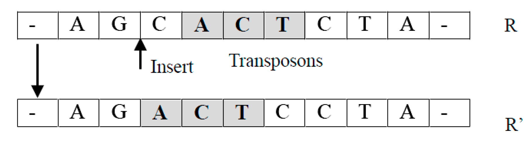
- Translocation operator TransLoc(R): It takes an individual as an input and returns a new individual by relocating a randomly selected unit of to a randomly chosen new location.For example, suppose , where is a unit. A new individual returned can be in which has been moved into the position before . Notice that it is easy to extend this operation so that an arbitrary new location can be selected (See Figure 2).
- (2)
- Transformation operator Transform(R): It takes an individual and two positions as parameters, and returns a new individual by swapping two randomly selected units.For example, the sequence becomes , after exchanging randomly selected units with .
- (3)
- Permutation operator Permute(R): It takes an individual as a parameter, and returns a new individual in which a randomly selected unit is randomly permuted.For example, if , the new individual can be , where is a random permutation of a randomly selected unit .
3.2. Mutation Operations
Mutation operators are used to mimic mutations in DNA replication caused by mutagens such as chemical agents and radiation. A mutation operator will make random changes to the structure of an individual. These operators will be used to increase the diversity of the population and to prevent the algorithm from converging to local optima. Here, we introduce three new mutation operators which are performed according to a pre-specified probability .
- (1)
- Inverse anticodon mutation IA(R). It takes an individual as a parameter and returns a new individual by replacing a randomly selected unit (as a codon) with its inverse anticodon. In biology, the anticodon of a codon is obtained by replacing each nucleotide with its complementary nucleotide based on the Watson–Crick complementary principle. Thus, A is replaced by T, C by G, and vice versa. An inversed anticodon is obtained by inverting the nucleotide sequence of the anticodon.For example, if the randomly selected codon is GCA (or 112 in numerical code), its anticodon will be CCT (or 003 in coding) and its inverse anticodon is TCC (or 300 in coding).
- (2)
- Frequency mutation FM(R). It takes an individual as a parameter and returns a new individual by replacing every occurrence of the most frequently appearing nucleotide by the least frequently appearing nucleotide.For example, in Figure 3 nucleotide G (represented by 1) is the most frequently appearing and nucleotide C (represented by 0) is the least frequently appearing. Thus, the FM operator replaces every G using a C.
- (3)
- Pseudo-bacteria mutation Pseudobac(R). It takes an individual as a parameter and returns a new individual as follows.First, a random subsequence of nucleotides is identified as a gene. Then, a given number of candidate individuals are created by randomly changing one nucleotide in the selected gene. Finally, the candidate individual with the highest fitness value is returned.For example, in Figure 4, gene1 is randomly selected, and five variations are created by changing one nucleotide at a time (indicated by the shaded bold letter). One candidate individual is created by using each of the variants to replace gene1.
This operator mimics a type of bacterial infection which, in a biological sense, may result in a new individual with an improved quality. The design is inspired by the pseudo-bacteria algorithm proposed by Yoshikawa et al. [27].
3.3. Recombination Operation
The recombination operator Recomb(R1, R2) performs two sub-tasks: cutting the molecules by restriction enzymes and pasting together the molecules obtained, provided that they have matching sticky ends. It is designed based on the splicing model described by Amos and Paun [28]. This operation is performed according to another pre-specified probability .
For each individual, a double-strand DNA is created from its single-strand DNA according to the complementary property of the nucleotides (i.e., A and T, and C and G are complementary to each other).
For example, suppose R1 = CCCCCTCGACCCCC and R2 = AAAAGCGCAAAA, the following double-stranded DNA molecules will be created:

Restriction enzymes can act upon DNA sequences as chemical compounds able to recognize specific subsequences of DNA and to cut the DNA sequence at that place. For instance, the enzymes named TaqI and SciNI are characterized by the recognition sequences:
![Algorithms 10 00076 i001]() respectively. The restriction enzymes TaqI and SciNI will cleave the above two molecules R1 and R2 into four segments:
respectively. The restriction enzymes TaqI and SciNI will cleave the above two molecules R1 and R2 into four segments:
 respectively. The restriction enzymes TaqI and SciNI will cleave the above two molecules R1 and R2 into four segments:
Notice the uneven cuts of the segments. Specifically, from left to right, the first and the fourth segments have complementary leads (the top and the bottom strands contain complementary nucleotides), and so do the second and the third segments. Next, the segments with complementary leads are combined into new double-strands. For the given example, the new double-strands are as follows:

Finally, the two top strands, CCCCCTCGAAAAA and AAAAGCGCCCCC, are returned as two new individuals.
4. The GA-TNE+DRO Algorithm
In this section, we present a genetic algorithm that used the triplet nucleotide coding in Section 2 and the genetic operations in Section 3.
In GA-TNE+DRO, we introduce the simulated annealing method. At the end of each generation, it compares the current best individual with previous ones. If the current optimum is improved, nothing will be done. Otherwise, GA-TNE+DRO (Algorithm 1) will randomly generate some (e.g., 10) individuals in the nearby area. We compare the fitness values among them and pick the best one as the current generation optimum.
| Algorithm 1 GA-TNE+DRO |
| Input: : the objective function : the number of variables in : domains of the n variables : the size of initial population Pc: the probability of crossover operation Pm: the probability of mutation operation Pr: the probability of recombination operation : max number of iterations : accuracy threshold Output: The value of X that optimizes Method: 1. POP = a population of randomly generated individuals 2. For each p in POP 3. Calculate the fitness value of p using f(decode(p)) 4. = the best individual in POP 5. OldX = any individual in POP that is not 6. While termination condition is not satisfied do 7. OldX = 8. NewPOP = {} 9. NEU = {N/2 neutral individuals in POP} 10. DEL = {N/2 deleterious individuals in POP} 11. For each individual p in NEU 12. Apply crossover operations to p according to Pc and add results to NewPOP 13. For each individual p in DEL 14. Apply mutation operations to p according to Pm and add results to NewPOP 15. For each pair of individual p and p’ in POP 16. Apply the recombination operation according to Pr and add results to NewPOP 17. For each p in NewPOP 18. Calculate the fitness value of p using f(decode(p)) 19. = the best individual in NewPOP 20. If is not better than OldX then 21. Generate randomly new individuals and pick up the best one into NewPOP 22. POP = NewPOP 23. End while 24. Return decode (X) |
This algorithm explores the solution space iteratively to find the optimal global solutions to a given optimization problem. The input parameters define the optimization problem with the objective function, number of variables and the domains of each variable, and the probabilities for applying various types of operators.
In Step 1, an initial population of N individuals is randomly created. Each individual is a sequence of variables encoded by the encoding method presented in Section 2. In Steps 2 and 3, a fitness value is calculated for each individual using the objective function on the decoded values of the variables. The current optimal individual is identified in Step 4. Within each iteration (in Step 7 through Step 22), the current best individual is directly passed into the next generation in Step 8. This is based on the elitism strategy [29], so that the individuals with the highest fitness values are always kept in the population.
In Steps 9 and 10, the neutral and deleterious individuals in the current population are identified. According to the DNA model [30], neutral individuals should have high fitness values and are likely to generate better solutions in the genetic process; deleterious individuals will not affect the final solutions, but they can help maintain or increase the diversity of the population. We use a tournament selection strategy to identify neutral and deleterious individuals. Assume that the current population has N individuals. First, we randomly select two individuals and keep the one with the higher fitness value as a neutral individual. We repeat this process until ceiling (N/2) neutral individuals have been selected. We then randomly create ceiling (N/2) new individuals for the current population. The same procedure is applied to select ceiling (N/2) deleterious individuals, only this time, the individual with a lower fitness value is selected.
The translocation, transformation, and permutation operators are then randomly applied to each neutral individual in Step 12 according to Pc, the probability of crossover operations. The mutation, inverse anticodon mutation, frequency mutation, and pseudo-bacteria mutation operators are then randomly applied to each deleterious individual in Step 14 according to Pm, the probability of mutation operations. Next, the recombination operation is randomly applied to each pair of individuals of the population in Step 16 according to Pr, the probability of recombination operations. New individuals created by the crossover, mutation, and recombination operations are added to the new population. At the end of each iteration, if the fitness value of the optimal individual is not improved, some (e.g., 10) additional individuals will be randomly generated to prevent the search from being trapped in a local optimum. In Step 22, the old population is replaced by the new population.
The process will terminate after Step 22 if the maximum number of iterations G has been reached or the improvement of the fitness values between the old and the new optimal individuals is not larger than , which is the user specified threshold. Finally, the optimal solution is returned in Step 24.
5. Numerical Experiments
In this section, we first describe our experiments and discuss the results. Then, we provide the algorithm complexity.
5.1. Experiment Setup
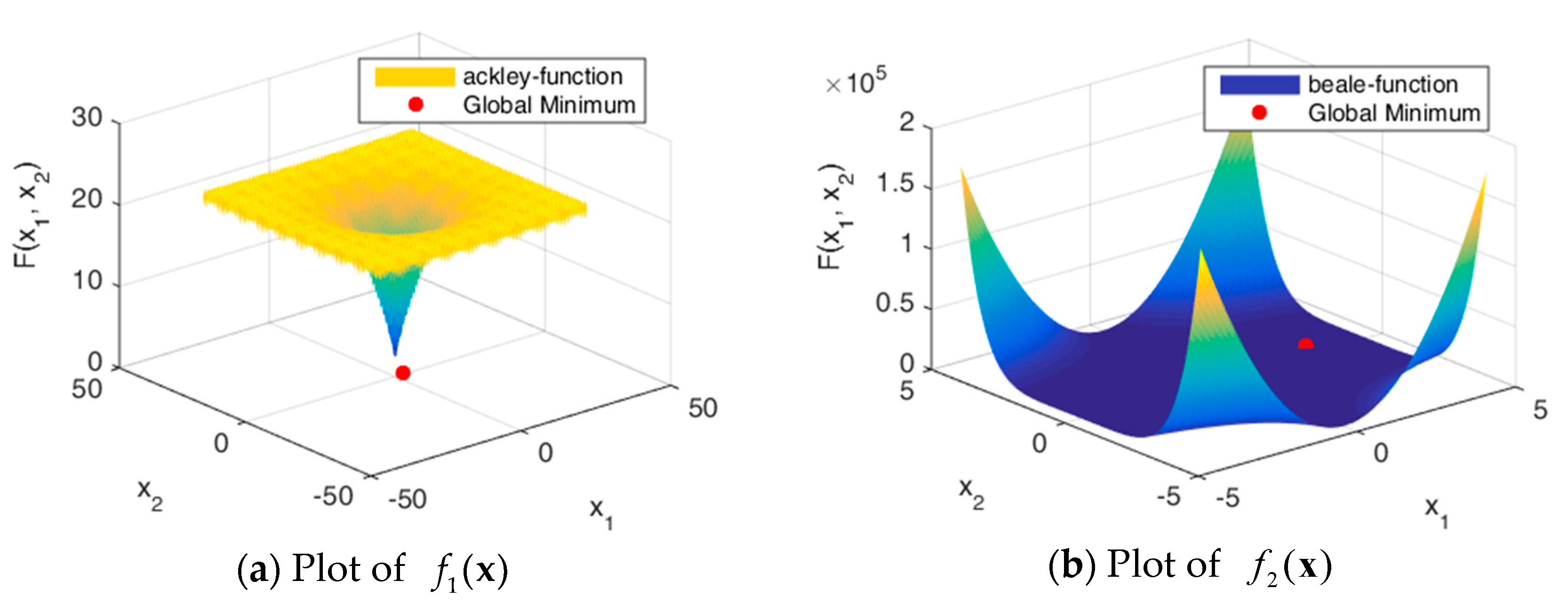
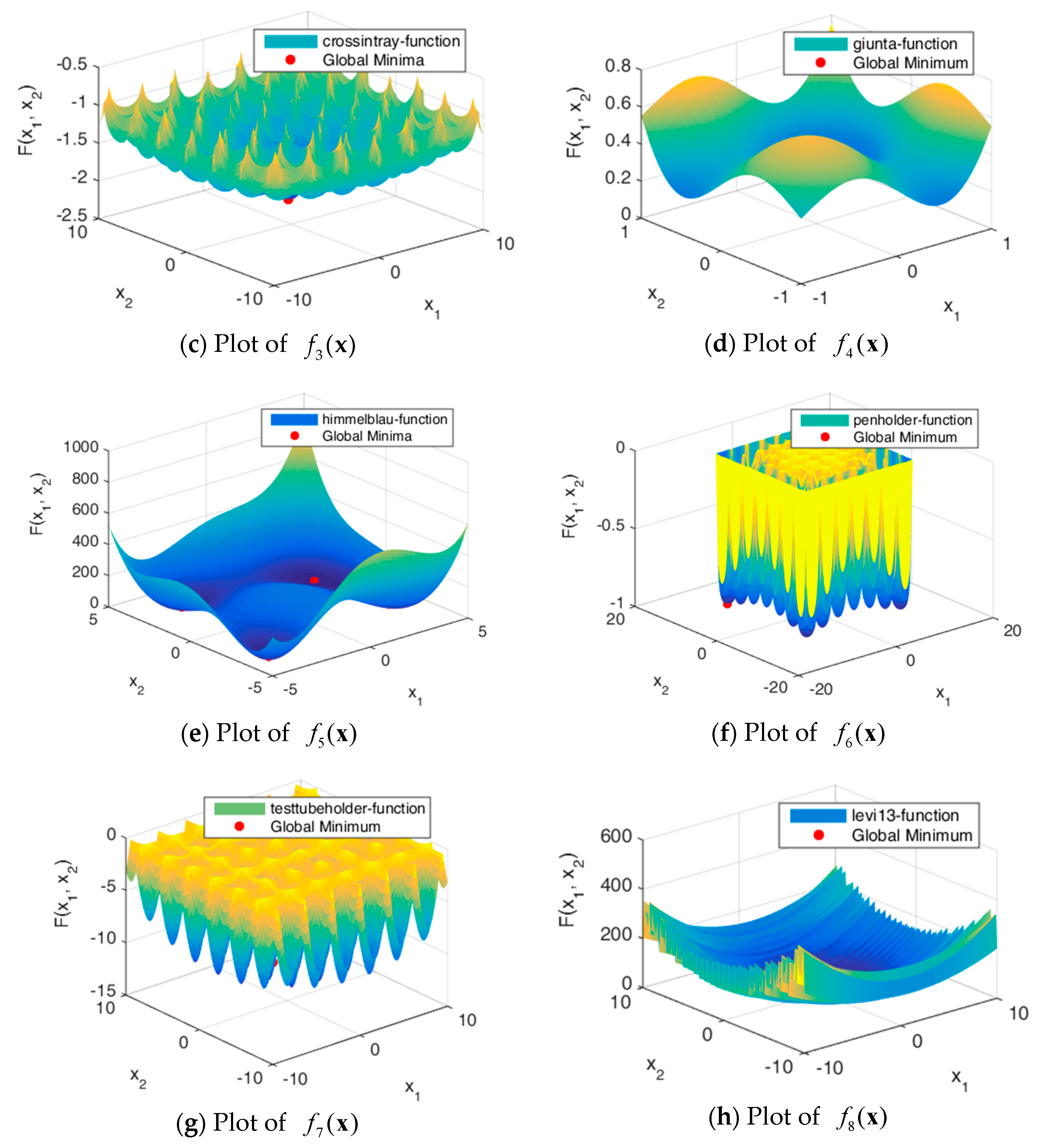
We implemented four algorithms: GA-TNE+NRO, conventional GA [1], PSO [2], and DE [3] in MATLAB and ran our experiment on a laptop with 4-core CPU in Windows 7. We applied these algorithms on a benchmark of eight nonlinear unconstrained optimization problems that are commonly used to evaluate the performance of global optimization algorithms [31]. These problems are difficult to solve using conventional optimization algorithms due to their large search space, numerous local minima, and fraudulence. Table 2 summarizes these optimization problems. For convenience, we refer to the optimization problems in Table 2 by their objective functions through .
Figure 5 shows the solution spaces of these problems. Problems through are uni-modal, which have precisely one global optimum, and are good for studying how well the algorithm can exploit the solution space [32]. Problems through are multimodal, which have one global optimum and many local optima. The number of local optima will increase exponentially as the number of dimensions increases.
Table 3 lists the set of parameters we used to run the algorithms on the benchmark problems. Here, denotes the number of iterations, N is the size of the initial population, Pc is the probability of crossover operations, Pm is the probability of mutation operations, and Pr is the probability of recombination operations.
For impartial comparison, each algorithm is executed 50 times for every benchmark problem. For each run, the optimization process terminates if , where denotes the best optimized objective function value, is the real optimal value, and is the precision threshold.
5.2. Results and Discussion
We compared the performance of the algorithms by comparing the values of the objective function and the number of iterations for the algorithms to converge.
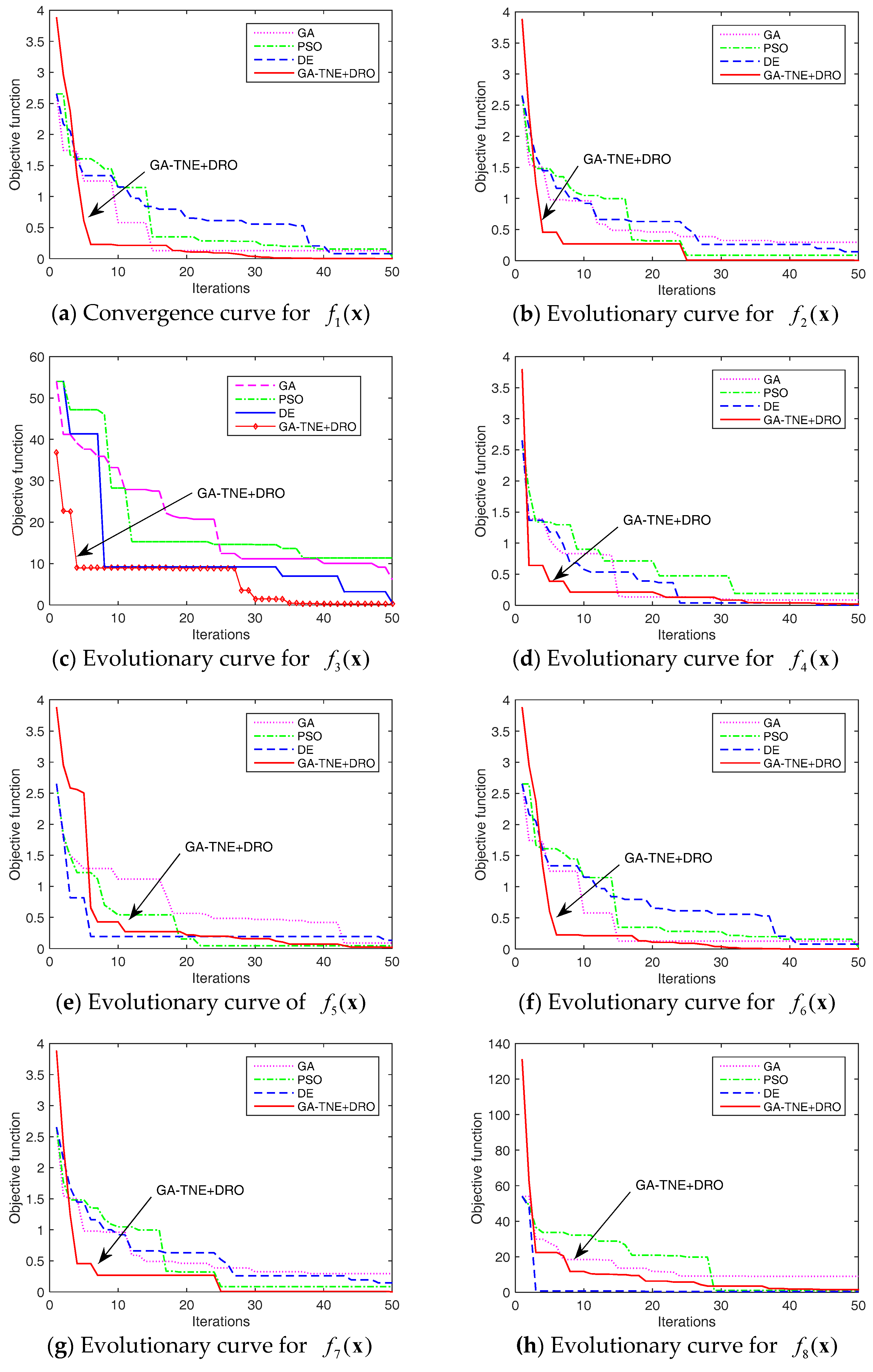
Figure 6 shows the evolution curves of the algorithms for each benchmark problem. For the sake of clarity, only 50 iterations are shown in Figure 6. Although a maximum of 1000 iterations were run in our experiments, the objective values stay unchanged beyond 50 iterations. As shown in Figure 6, our algorithm can find better solutions earlier than other algorithms for most of the benchmark problems.
Table 4 shows the ability of the algorithms to find the global optimal solutions. Notice that since all benchmark problems require the objective functions to be minimized, the smaller the value of the objective function for the solution obtained by the algorithm, the more accurate the solution is. In Table 4, the columns labeled with and are, respectively, the average and best values of the objective function at the termination of the algorithm over 50 runs. The best obtained results are highlighted in bold.
From these results, we can see that our algorithm outperforms the other algorithms in all benchmark problems, except for in both the average and the optimal cases. This clearly indicates that our algorithm can find solutions that are much closer to the global optimal solution than other algorithms, especially for optimization problems in high dimensional space. The slightly worse performance than DE for problem was due to the difficulty caused by thousands of local optima in the solution space. However, this result of our algorithm is still much better than those of GA and PSO.
Table 5 shows the speed at which the algorithms converge. We measured the maximum, minimum, and average number of iterations executed until the algorithms converged to a solution.
From Table 5, we can see that our algorithm converges much faster than other algorithms on all benchmark problems except .
5.3. Algorithm Complexity
In this Section, the algorithm complexity for the proposed GA-TNE+DRO is described. Table 6 shows the complexity of the four algorithms: GA, PSO, DE, and GA-TNE+DRO. Using the method in [33], the running times of algorithms are measured against , the running time of Algorithm 2. Under our experimental setup, is 3.4 × 10⁻⁵ s.
| Algorithm 2 Test Problem |
| for i = 1:200 x = 0.55 + i; x = x + x; x = x/ 2; x = x*x; x= sqrt(x); x = log(x); x= exp(x); x = x/(x+2); end |
In Table 6, is the running time for executing the benchmark function alone for 200 times. is the total running time for applying an algorithm to solve a benchmark function 200 times. is the mean over 50 runs. The complexity of the algorithm is measured by . The best results in Table 6 are highlighted in bold. According to Table 6, our algorithm is much more efficient than the other algorithms.
6. Conclusions
To accelerate the evolutionary process and increase the probability to find the optimal solution, we present a new genetic algorithm, called GA-TNE+DRO, which uses a novel triplet nucleotide coding scheme to encode potential solutions and a set of new genetic operators to search for globally optimal solutions. The coding scheme represents potential solutions as a sequence of triplet nucleotides and the DNA reproduction operations mimic the DNA reproduction process more vividly than existing DNA-GAs. We compared our algorithm with several existing GA and DNA-based GA algorithms using a benchmark of eight optimization functions. Our experimental results show that our algorithm can converge to solutions much closer to the global optimal solutions in a much lower number of iterations than the existing algorithms.
Several interesting issues may deserve further research. It may be interesting to explore a new encoding scheme and new genetic operators for a better performance and efficiency. The current algorithm is designed for solving unconstrained optimizations; however, it would be interesting to extend this algorithm to solve other types of optimizations, for example, constrained optimization and multi-objective optimization problems. It would also be interesting to apply the algorithm to solve problems in machine learning, such as clustering and classification.
Acknowledgments
The work was done while the first author was visiting the University of Texas at San Antonio, USA. The authors would like to express thanks to the editor and the reviewers for their insightful suggestions. This research is supported in part by Excellent Young Scholars Research Fund of Shandong Normal University, China; the National Science Foundation of China (Nos. 61472231, 61402266); the Jinan Youth Science and Technology Star Project under Grant 20120108; and the soft science research on national economy and social information of Shandong, China under Grant (2015EI013).
Author Contributions
All four authors made significant contributions to this research. Together, they conceived the ideas, designed the algorithm, performed the experiments, analyzed the results, drafted the initial manuscript, and revised the final manuscript.
Conflicts of Interest
The authors declare no conflict of interest.
References
- Holland, J.H. Adaptation in Natural and Artificial Systems; University of Michigan Press: Ann Arbor, MI, USA, 1975. [Google Scholar]
- Guedria, N.B. Improved accelerated PSO algorithm for mechanical engineering optimization problems. Appl. Soft Comput. 2016, 40, 455–467. [Google Scholar] [CrossRef]
- Storn, R.; Price, K. Differential Evolution—A simple and efficient heuristic for global optimization over continuous spaces. J. Glob. Optim. 1997, 11, 341–359. [Google Scholar] [CrossRef]
- Garg, H. Solving structural engineering design optimization problems using an artificial bee colony algorithm. J. Ind. Manag. Optim. 2014, 10, 777–794. [Google Scholar] [CrossRef]
- Garg, H.; Sharma, S.P. Multi-objective reliability redundancy allocation problem using particle swarm optimization. Comput. Ind. Eng. 2013, 64, 247–255. [Google Scholar] [CrossRef]
- Fan, Q.; Yan, X. Self-adaptive differential evolution algorithm with discrete mutation control parameters. Expert Syst. Appl. 2015, 42, 1551–1572. [Google Scholar] [CrossRef]
- Garg, H. A hybrid GA-GSA algorithm for optimizing the performance of an industrial system by utilizing uncertain data. In Handbook of Research on Artificial Intelligence Techniques and Algorithms; IGI Global: Hershey, PA, USA, 2015; pp. 620–654. [Google Scholar]
- Pelusi, D.; Mascella, R.; Tallini, L. Revised gravitational search algorithms based on evolutionary-fuzzy systems. Algorithms 2017, 10, 44. [Google Scholar] [CrossRef]
- Garg, H. A hybrid PSO-GA algorithm for constrained optimization problems. Appl. Math. Comput. 2016, 274, 292–305. [Google Scholar] [CrossRef]
- Garg, H. An efficient biogeography based optimization algorithm for solving reliability optimization problems. Swarm Evol. Comput. 2015, 24, 1–10. [Google Scholar] [CrossRef]
- Adleman, L.M. Molecular computation of solutions to combinatorial problems. Science 1994, 266, 1021–1024. [Google Scholar] [CrossRef] [PubMed]
- Nabil, B.; Guenda, K.; Gulliver, A. Construction of codes for DNA computing by the greedy algorithm. ACM Commun. Comput. Algebra. 2015, 49. [Google Scholar] [CrossRef]
- Mayukh, S.; Ghosal, P. Implementing Data Structure Using DNA: An Alternative in Post CMOS Computing. In Proceedings of the 2015 IEEE Computer Society Annual Symposium on VLSI, Montpellier, France, 8–10 July 2015. [Google Scholar]
- Huang, Y.; Tian, Y.; Yin, Z. Design of PID controller based on DNA COMPUTING. In Proceedings of the International Conference on Artificial Intelligence and Computational Intelligence (AICI), Sanya, China, 23–24 October 2010; pp. 195–198. [Google Scholar]
- Yongjie, L.; Jie, L. A feasible solution to the beam-angle-optimization problem in radiotherapy planning with a DNA-based genetic algorithm. IEEE Trans. Biomed. Eng. 2010, 57, 499–508. [Google Scholar] [CrossRef] [PubMed]
- Damm, R.B.; Resende, M.G.; Débora, P.R. A biased random key genetic algorithm for the field technician scheduling problem. Comput. Oper. Res. 2016, 75, 49–63. [Google Scholar] [CrossRef]
- Li, H.B.; Demeulemeester, E. A genetic algorithm for the robust resource leveling problem. J. Sched. 2016, 19, 43–60. [Google Scholar] [CrossRef]
- Ding, Y.S.; Ren, L.H. DNA genetic algorithm for design of the generalized membership-type Takagi-Sugeno fuzzy control system. In Proceedings of the 2000 IEEE International Conference on Systems, Man, and Cybernetics, Nashville, TN, USA, 8–11 October 2000; pp. 3862–3867. [Google Scholar]
- Zhang, L.; Wang, N. A modified DNA genetic algorithm for parameter estimation of the 2-chlorophenol oxidation in supercritical water. Appl. Math. Model. 2013, 37, 1137–1146. [Google Scholar] [CrossRef]
- Chen, X.; Wang, N. Optimization of short-time gasoline blending scheduling problem with a DNA based hybrid genetic algorithm. Comput. Chem. Eng. 2010, 49, 1076–1083. [Google Scholar] [CrossRef]
- Zhang, L.; Wang, N. An adaptive RNA genetic algorithm for modeling of proton exchange membrane fuel cells. Int. J. Hydrog. Energy 2013, 38, 219–228. [Google Scholar] [CrossRef]
- Zang, W.K.; Sun, M.H.; Jiang, Z.N. A DNA genetic algorithm inspired by biological membrane structure. J. Comput. Theor. Nanosci. 2016, 13, 3763–3772. [Google Scholar] [CrossRef]
- Sun, Z.; Wang, N.; Bi, Y. Type-1/type-2 fuzzy logic systems optimization with RNA genetic algorithm for double inverted pendulum. Appl. Math. Model. 2015, 39, 70–85. [Google Scholar] [CrossRef]
- Zang, W.K.; Ren, L.Y.; Zhang, W.Q.; Liu, X.Y. Automatic density peaks clustering using DNA genetic algorithm optimized data field and Gaussian process. Int. J. Pattern Recognit. Artif. Intell. 2017, 31, 1750023. [Google Scholar] [CrossRef]
- Zang, W.K.; Jiang, Z.N.; Ren, L.Y. Spectral clustering based on density combined with DNA genetic algorithm. Int. J. Pattern Recognit. Artif. Intell. 2017, 31, 7799. [Google Scholar] [CrossRef]
- Zang, W.K.; Sun, M.H. Searching parameter values in support vector machines using DNA genetic algorithms. Lect. Notes Comput. Sci. 2016, 9567, 588–598. [Google Scholar]
- Yoshikawa, T.; Furuhashi, T.; Uchikawa, Y. The effects of combination of DNA coding method with pseudo-bacterial GA. In Proceedings of the 1997 IEEE International Conference on Evolutionary Computation, Indianapolis, IN, USA, 13–16 April 1997; pp. 285–290. [Google Scholar]
- Amos, M.; Păun, G.; Rozenberg, G.; Salomaa, A. Topics in the theory of DNA computing. Theor. Comput. Sci. 2002, 287, 3–38. [Google Scholar] [CrossRef]
- Cheng, W.; Shi, H.; Xin, X.; Li, D. An elitism strategy based genetic algorithm for streaming pattern discovery in wireless sensor networks. Commun. Lett. IEEE 2011, 15, 419–421. [Google Scholar] [CrossRef]
- Neuhauser, C.; Krone, S.M. The genealogy of samples in models with selection. Genetics 1997, 145, 519–534. [Google Scholar] [PubMed]
- Haupt, R.L.; Haupt, S.E. Practical Genetic Algorithms, 2nd ed.; John Wiley & Sons, Inc.: Camp Hill, PA, USA, 2004. [Google Scholar]
- Mirjalili, S.; Mirjalili, S.M.; Hatamlou, A. Multi-verse optimizer: A nature inspired algorithm for global optimization. Neural Comput. Appl. 2015. [Google Scholar] [CrossRef]
- Liang, J.; Qu, B.; Suganthan, P. Problem Definitions and Evaluation Criteria for the CEC 2014 Special Session and Competition on Single Objective Real-Parameter Numerical Optimization; Technical Report; Computational Intelligence Laboratory, Zhengzhou University: Zhengzhou, China; Nanyang Technological University: Singapore, 2013. [Google Scholar]
Figure 1.
The coding for two variables.
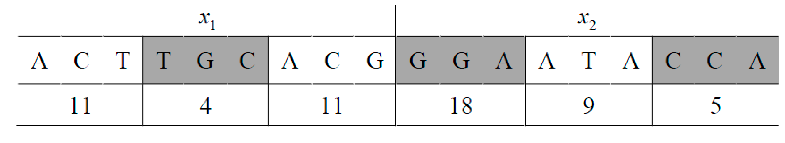
Figure 2.
Transposition operation process.

Figure 3.
An example of FM.
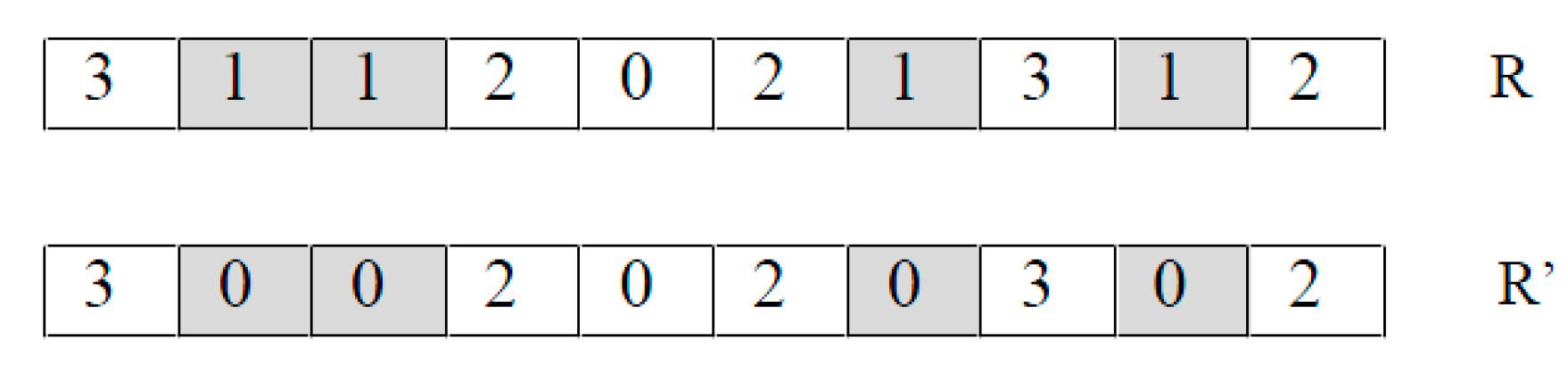
Figure 4.
Pseudo bacteria genetic operation diagram.
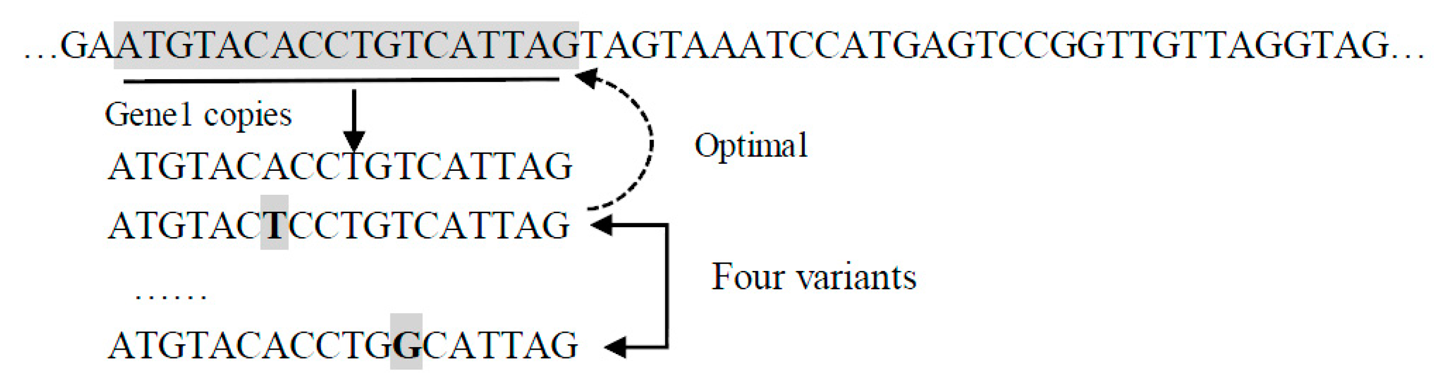
Figure 5.
Plots of benchmark functions.


Figure 6.
Evolution curves of benchmark functions.


Table 1.
Relationship between triplet codons and 19-ary integers.
| First Nucleotide | Second Nucleotide | Third Nucleotide | |||
|---|---|---|---|---|---|
| T | C | A | G | ||
| T | Phe(0) | Ser(2) | Tyr(3) | Cys(4) | T |
| T | Phe(0) | Ser(2) | Tyr(3) | Cys(4) | C |
| T | Leu(1) | Ser(2) | Stop(9) | Stop(9) | A |
| T | Leu(1) | Ser(2) | Stop(9) | Try(9) | G |
| C | Leu(1) | Pro(5) | His(6) | Arg(8) | T |
| C | Leu(1) | Pro(5) | His(6) | Arg(8) | C |
| C | Leu(1) | Pro(5) | Gln(7) | Arg(8) | A |
| C | Leu(1) | Pro(5) | Gln(7) | Arg(8) | G |
| A | Ile(10) | Thr(11) | Asn(12) | Ser(2) | T |
| A | Ile(10) | Thr(11) | Asn(12) | Ser(2) | C |
| A | Met(9) | Thr(11) | Lys(13) | Arg(8) | A |
| A | Met(9) | Thr(11) | Lys(13) | Arg(8) | G |
| G | Val(14) | Ala(15) | Asp(16) | Gly(18) | T |
| G | Val(14) | Ala(15) | Asp(16) | Gly(18) | C |
| G | Val(14) | Ala(15) | Glu(17) | Gly(18) | A |
| G | Val(14) | Ala(15) | Glu(17) | Gly(18) | G |
Table 2.
Benchmark functions.
| Function Name | Function Formula | Optimal Solution | Optimum |
|---|---|---|---|
| Ackley | [−3, 0.5] | 0 | |
| Beale | [−3, 0.5] | 0 | |
| Crossintray | [0.3459, 0.3459] | 0 | |
| Giunta | [−10, 10] | −20 | |
| Himmelblau | [3,2] | 0 | |
| Penholder | [−9.64617, 9.64617] | −0.96353 | |
| Testtubeholder | [, 0] | −10.8723 | |
| Levi13 | [1,1] | 0 |
Table 3.
Parameter setting for GA, PSO, DE, and GA-TNE+DRO.
| GA | PSO | DE | GA-TNE+DRO |
|---|---|---|---|
| G = 200 | G = 200 | G = 200 | G = 200 |
| N = 20 | N = 20 | N = 20 | N = 20 |
| Pc = 0.5 | C1 = 2, C2 = 2 | Pc = 0.5 | Pc = 0.5 |
| Pm = 0.01 | w1 = 0.9, w2 = 0.4 | Pm = 0.06 | Pm = 0.05, Pr = 0.05 |
Table 4.
The optimal values of objective functions obtained by the algorithms (the best obtained results are highlighted in bold).
Table 4.
The optimal values of objective functions obtained by the algorithms (the best obtained results are highlighted in bold).
| Function | GA | PSO | DE | GA-TNE+DRO | ||||
|---|---|---|---|---|---|---|---|---|
| 8.43 × 10⁻⁸ | 4.91 × 10⁻⁷ | 3.13 × 10⁻¹⁰ | 3.67 × 10⁻⁸ | 4.13 × 10⁻⁹ | 3.18 × 10⁻⁸ | 1.13 × 10⁻¹¹ | 1.16 × 10⁻¹⁰ | |
| 3.48 × 10⁻⁷ | 6.12 × 10⁻⁶ | 5.62 × 10⁻⁹ | 4.12 × 10⁻⁸ | 7.52 × 10⁻¹⁰ | 7.01 × 10⁻⁹ | 7.85 × 10⁻¹¹ | 8.61 × 10⁻¹⁰ | |
| 1.86 × 10⁻⁸ | 3.65 × 10⁻⁶ | 1.58 × 10⁻¹⁰ | 4.28 × 10⁻⁹ | 3.04 × 10⁻¹⁰ | 3.17 × 10⁻⁹ | 2.47 × 10⁻¹² | 3.45 × 10⁻¹¹ | |
| −20.0023 | −20.0238 | −19.9986 | −19.9865 | −19.9987 | −19.9928 | −20.0001 | −20.0010 | |
| 2.36 × 10⁻⁵ | 5.69 × 10⁻⁴ | 3.65 × 10⁻⁶ | 7.54 × 10⁻⁵ | 5.97 × 10⁻⁶ | 4.19 × 10⁻⁵ | 7.98 × 10⁻⁷ | 8.67 × 10⁻⁶ | |
| −0.96350 | −0.96251 | −0.96349 | −0.96332 | −0.96343 | −0.96341 | −0.96354 | −0.96350 | |
| −10.8716 | −10.8689 | −10.8718 | −10.8702 | −10.8718 | −10.8703 | −10.8721 | −10.8714 | |
| 4.35 × 10⁻⁸ | 2.36 × 10⁻⁶ | 3.68 × 10⁻⁹ | 6.39 × 10⁻⁷ | 8.26 × 10⁻¹⁰ | 8.69 × 10⁻⁹ | 6.31 × 10⁻⁹ | 9.23 × 10⁻⁸ | |
Table 5.
The Convergence Speed of the Algorithms (the best obtained results are highlighted in bold).
Table 5.
The Convergence Speed of the Algorithms (the best obtained results are highlighted in bold).
| Function | GA | PSO | DE | GA-TNE+DRO | ||||||||
|---|---|---|---|---|---|---|---|---|---|---|---|---|
| 200 | 54 | 86.8 | 200 | 51 | 65.8 | 191 | 50 | 70.4 | 180 | 9 | 15.6 | |
| 200 | 102 | 120.4 | 187 | 69 | 111.6 | 182 | 49 | 95.7 | 159 | 23 | 56.8 | |
| 198 | 118 | 142.6 | 168 | 87 | 115.6 | 174 | 37 | 61.7 | 149 | 19 | 24.6 | |
| 186 | 76 | 126.8 | 182 | 76 | 116.8 | 170 | 72 | 120.4 | 138 | 28 | 96.8 | |
| 178 | 78 | 125.6 | 186 | 42 | 87.6 | 158 | 62 | 111.3 | 127 | 26 | 75.6 | |
| 192 | 96 | 130.1 | 192 | 63 | 97.6 | 144 | 55 | 102.7 | 106 | 27 | 38.8 | |
| 187 | 112 | 168.3 | 193 | 61 | 91.3 | 162 | 28 | 75.8 | 116 | 19 | 50.2 | |
| 186 | 86 | 118.6 | 179 | 53 | 78.6 | 104 | 13 | 24.4 | 132 | 21 | 52.4 | |
Table 6.
Algorithm complexity (the best obtained results are highlighted in bold).
| Function | T1 | GA | PSO | DE | GA-TNE+DRO | ||||
|---|---|---|---|---|---|---|---|---|---|
| T | T | T | T | ||||||
| 4.3874 × 10⁻³ | 9.2735 × 10⁻³ | 143.71 | 5.6002 × 10⁻³ | 35.672 | 8.1046 × 10⁻³ | 109.33 | 5.2750 × 10⁻³ | 26.105 | |
| 3.8156 × 10⁻³ | 8.0649 × 10⁻³ | 124.98 | 7.0483 × 10⁻³ | 95.078 | 4.8704 × 10⁻³ | 31.023 | 4.5875 × 10⁻³ | 22.702 | |
| 7.6552 × 10⁻³ | 1.6180 × 10⁻² | 250.74 | 1.4141 × 10⁻² | 190.75 | 9.7714 × 10⁻³ | 62.241 | 9.2038 × 10⁻³ | 45.547 | |
| 7.9521 × 10⁻³ | 1.6808 × 10⁻² | 260.47 | 1.4689 × 10⁻² | 198.15 | 1.0150 × 10⁻² | 64.654 | 9.5607 × 10⁻³ | 47.313 | |
| 1.8687 × 10⁻³ | 3.9498 × 10⁻³ | 61.210 | 2.3853 × 10⁻³ | 15.194 | 3.4519 × 10⁻³ | 46.565 | 2.2467 × 10⁻³ | 11.119 | |
| 4.8976 × 10⁻³ | 1.0352 × 10⁻² | 160.42 | 6.2515 × 10⁻³ | 39.821 | 9.0470 × 10⁻³ | 122.04 | 5.8884 × 10⁻³ | 29.14 | |
| 4.4559 × 10⁻³ | 9.4182 × 10⁻³ | 145.95 | 8.2309 × 10⁻³ | 111.03 | 5.6877 × 10⁻³ | 36.229 | 5.3573 × 10⁻³ | 26.512 | |
| 6.4631 × 10⁻³ | 1.3661 × 10⁻² | 211.70 | 1.1939 × 10⁻² | 161.05 | 7.7706 × 10⁻³ | 38.455 | 8.2498 × 10⁻³ | 52.549 | |
© 2017 by the authors. Licensee MDPI, Basel, Switzerland. This article is an open access article distributed under the terms and conditions of the Creative Commons Attribution (CC BY) license (http://creativecommons.org/licenses/by/4.0/).
Share and Cite
MDPI and ACS Style
Zang, W.; Zhang, W.; Zhang, W.; Liu, X. A Genetic Algorithm Using Triplet Nucleotide Encoding and DNA Reproduction Operations for Unconstrained Optimization Problems. Algorithms 2017, 10, 76. https://doi.org/10.3390/a10030076
AMA Style
Zang W, Zhang W, Zhang W, Liu X. A Genetic Algorithm Using Triplet Nucleotide Encoding and DNA Reproduction Operations for Unconstrained Optimization Problems. Algorithms. 2017; 10(3):76. https://doi.org/10.3390/a10030076
Chicago/Turabian StyleZang, Wenke, Weining Zhang, Wenqian Zhang, and Xiyu Liu. 2017. "A Genetic Algorithm Using Triplet Nucleotide Encoding and DNA Reproduction Operations for Unconstrained Optimization Problems" Algorithms 10, no. 3: 76. https://doi.org/10.3390/a10030076
Note that from the first issue of 2016, this journal uses article numbers instead of page numbers. See further details here.