Auxiliary Model Based Multi-Innovation Stochastic Gradient Identification Algorithm for Periodically Non-Uniformly Sampled-Data Hammerstein Systems

1
Key Laboratory of Advanced Process Control for Light Industry (Ministry of Education), Jiangnan University, Wuxi 214122, China
2
School of Internet of Things Engineering, Jiangnan University, Wuxi 214122, China
*
Author to whom correspondence should be addressed.
Algorithms 2017, 10(3), 84; https://doi.org/10.3390/a10030084
Submission received: 12 May 2017
/
Revised: 7 July 2017
/
Accepted: 19 July 2017
/
Published: 31 July 2017
Abstract
:Due to the lack of powerful model description methods, the identification of Hammerstein systems based on the non-uniform input-output dataset remains a challenging problem. This paper introduces a time-varying backward shift operator to describe periodically non-uniformly sampled-data Hammerstein systems, which can simplify the structure of the lifted models using the traditional lifting technique. Furthermore, an auxiliary model-based multi-innovation stochastic gradient algorithm is presented to estimate the parameters involved in the linear and nonlinear blocks. The simulation results confirm that the proposed algorithm is effective and can achieve a high estimation performance.
1. Introduction
The dynamics of most practical systems are inherently nonlinear due to complex physical, chemical and biological mechanisms. The modeling of nonlinear systems is challenging and has become an active research area in both academia and industry [1,2]. To simplify the modeling problem, block-oriented models, which are composed of linear dynamic blocks in combination with nonlinear memoryless blocks, have been widely utilized to describe nonlinear systems. The state of the art in designing, analyzing and implementing identification algorithms for block-oriented nonlinear systems were well summarized in a recent book by Giri and Bai [3]. Depending on the location of the static nonlinear component, block-oriented models can be classified into the Hammerstein model, the Wiener model and the Hammerstein–Wiener model [4,5,6]. The Hammerstein model represents a class of input nonlinear systems, where the nonlinear block is prior to the linear one. It can flexibly approximate various input nonlinearities, such as saturation, dead zone, backlash and hysteresis, thus having been extensively employed in realistic applications [7,8,9,10,11].
For decades, the identification of Hammerstein nonlinear systems has attracted much attention, and numerous methods have been reported in the literature. For example, Pouliquen et al. studied the parameter estimation of Hammerstein systems where the linear part is described by an output error model and presented an iterative algorithm based on the optimal bounding ellipsoid criterion [12]. Ding et al. applied the auxiliary model identification principle to deal with unmeasurable noise-free outputs in Hammerstein output error systems, presented a recursive least squares (RLS) algorithm and investigated its convergence properties [13]. Filipovic derived a robust extended RLS algorithm to estimate the parameters of Hammerstein systems interfered by non-Gaussian disturbance [14]. Gao et al. proposed a blind identification algorithm for Hammerstein systems with hysteresis nonlinearity and further developed a composite control strategy to track the reference input [15].
Among various new methodologies in the identification area, the multi-innovation theory has been considered as a useful way to improve estimation precision and convergence rate. The basic idea of the multi-innovation theory is innovation expanding, which helps to update the parameter estimates at each recursion using the data over a moving and fixed-size window [16,17]. Typically, the multi-innovation theory is incorporated with the RLS algorithm, the stochastic gradient (SG) algorithm, the stochastic Newton recursive algorithm, etc., to address identification problems [18]. For instance, a multi-innovation RLS algorithm was developed for Hammerstein AutoRegressive eXogenous (ARX) systems with backlash nonlinearity [19]. Furthermore, a multi-innovation SG algorithm [20] and an auxiliary model-based multi-innovation generalized extended SG algorithm [21] were proposed to estimate the parameters of Hammerstein nonlinear ARX and Box–Jenkins systems, respectively. Compared with the multi-innovation RLS algorithm, the multi-innovation SG algorithm is more efficient in computation because it avoids performing large matrix inversion [22].
The above-mentioned Hammerstein systems all belong to single-rate systems, the inputs and outputs of which are uniformly sampled at the same rate. However, non-uniform sampling can be encountered in practice due to hardware limitations or economic considerations [23,24,25]. For example, influenced by transmission delays and packet losses, the input-output data in networked control systems might be available at non-uniformly spaced time instants [26,27]. The non-uniform sampling includes the uniform sampling as its special case, which can always preserve controllability and observability in discretization [28]. Furthermore, it can overcome the restriction of the Nyquist limit and enable a much lower average sampling frequency. Therefore, intentional non-uniform sampling has the potential to reduce the hardware cost in control applications [29]. Due to the complexity of arbitrary non-uniform sampling, most of the literature works have focused on periodically non-uniformly sampled-data systems [30,31]. For periodically non-uniformly sampled-data Hammerstein systems, Li et al. derived the lifted transfer function model by means of the lifting technique and presented a least squares-based iterative algorithm for parameter estimation [32]. The lifting technique is a benchmark tool to deal with multirate and non-uniformly sampled-data systems [33,34]. However, the corresponding lifted models are complex and involve a large number of parameters, which brings a great challenge for identification. To simplify the model structure and reduce the identification complexity, Xie et al. put forward a novel input-output representation of linear systems with non-uniform sampling by introducing a time-varying backward shift operator [35]. On the basis of that work, this paper aims to propose a -based model to describe periodically non-uniformly sampled-data Hammerstein systems and presents an auxiliary model-based multi-innovation SG algorithm to estimate the model parameters.
The rest of this paper is organized as follows. Section 2 formulates the identification problem of periodically non-uniformly sampled-data Hammerstein systems. Identification algorithms are proposed in Section 3, and an example is provided in Section 4 to examine their estimation performance. Finally, concluding remarks are given in Section 5.
2. Problem Description
Consider a periodically non-uniformly sampled-data Hammerstein system as depicted in Figure 1, in which is a periodic non-uniform zero-order hold, converting a discrete-time input sequence to a continuous-time input , i.e.,
where ; T is the frame period spaced by q non-uniform sampling instants ().
By passing through a nonlinear static block , is transformed into an unmeasurable inner input to a linear dynamic process P with order n, which can be expressed as:
where are known nonlinear basis functions and are unknown coefficients to be estimated.
The noise-free output of the process P is corrupted by a white noise , generating a measurable output . The non-uniform sampler has a synchronous sampling pattern with ; thus, the discrete-time output sequence is obtained at sampling instants ().
For the notational simplicity, in the following the data , at non-uniform sampling time , is denoted by . By using a time-varying backward shift operator proposed in [35], the mapping relationship between the inner input and the noise-free output of the periodically non-uniformly sampled-data Hammerstein system can be represented as:
where:
From the system schematic diagram in Figure 1, we have:
3. Identification Algorithms
3.1. The AM-SG Algorithm
According to the over-parameterized linear regression approach [36], define the information vector and the parameter vector as:
Substituting Equation (4) into Equation (3), we have:
Equation (5) is the identification model of the periodically non-uniformly sampled-data Hammerstein system, in which the parameter vector includes the products of parameters and . To guarantee a unique parametrization, the first coefficient of the nonlinear function is assumed to be one [14,37]. Furthermore, the information vector contains unmeasurable noise-free outputs . A solution to this difficulty is to replace with their estimates based on the auxiliary model identification idea [38,39,40]. Accordingly, define the estimate of as:
Using the estimates and to replace and in (4), respectively, yields
Applying the stochastic gradient search principle to minimize the following criterion function:
an auxiliary model-based stochastic gradient (AM-SG) algorithm can be derived for identifying the parameter vector in (5):
3.2. The AM-MISG Algorithm
The AM-SG algorithm only uses the current dataset to update the parameter estimates. Therefore, it has a slow convergence rate and low estimation accuracy. To improve the identification performance of the AM-SG algorithm, an innovation length p is introduced to derive an auxiliary model-based multi-innovation stochastic gradient (AM-MISG) algorithm.
Considering the most recent p sets of input-output data, define the stacked output vector , the stacked noise vector and the stacked information matrix as:
Equation (5) can be expanded into the following matrix form:
However, the information vectors in include unknown noise-free outputs. Let be their estimates; the estimate of can be defined as:
Define the following criterion function:
where represents the norm of the matrix X. The gradient of with respect to is given by:
Applying the stochastic gradient search principle to minimize the criterion function in (10), we have:
where is called the step size or the convergence factor. For the convenience of formula derivation, let ; Equation (11) can be rewritten into:
To guarantee the convergence of this recursive algorithm, all eigenvalues of the matrix should be located inside the unit circle. Therefore, a conservative choice of is:
In this paper, we take a common choice:
where is the forgetting factor.
Substituting Equation (13) into Equation (12), the auxiliary model-based multi-innovation stochastic gradient (AM-MISG) algorithm can be derived:
Since , the estimates of and can be directly read from ,
where represents the j-th element of . Note that () has been estimated times at each non-uniform sampling instant (). Therefore, we can simply take their average like in [36] as the estimate of over the k-th frame period, i.e.,
Furthermore, a more numerically-sound SVD-based approach proposed by Bai [41] can be applied to obtain the estimates of and .
The flowchart of the AM-MISG algorithm in (14)–(25) for computing the parameter estimates of periodically non-uniformly sampled-data Hammerstein systems can be illustrated in Figure 2, and the detailed implementation steps are summarized as follows:
- Initialization: Choose the data length L, the innovation length p and the forgetting factor ; give the nonlinear basis functions ; set , , for and ; take the initial values to be , where and is a column vector of ones; let and .
- Collect the non-uniformly sampled input-output data and .
- Calculate based on ; form , , by (19)–(21); and construct by (18).
- Form the stacked output vector and the stacked information matrix by (16) and (17), respectively.
- Compute the step size by (15) and update the parameter estimate by (14); calculate by (22); obtain and based on (23) and (24), respectively.
- If , then increase i by one, and go to Step 2; otherwise, compute by (25); let and go to the next step.
- If , then increase k by one, and go to Step 2; otherwise, terminate the computing process.
3.3. The Main Convergence Result
The main convergence result of the proposed AM-MISG algorithm for periodically non-uniformly sampled-data Hammerstein systems is given in the following theorem.
Theorem 1.
Assume that the noise sequences satisfy:
- (A1)
and there exist a positive constant α and an integer N such that the following persistent excitation condition holds:
- (A2)
Then, the parameter estimation vector given by the AM-MISG algorithm consistently converges to the true parameter vector in the mean-square sense.
Theorem 1 can be proven in a similar way to [42]. Therefore, its detailed proof is omitted here.
4. Simulation Example
Assume that the nonlinear block in Figure 1 is described by:
and the linear continuous process P is described by:
Over a frame period of s, the input-output data are non-uniformly-sampled twice (i.e., ) at s and s. According to Theorem 1 in [35], the following -based transfer function model is derived:
Therefore, the parameters of this periodically non-uniformly sampled-data Hammerstein system are:
In the simulation, take the non-uniform inputs and as two uncorrelated random sequences with zero mean and unit variance, and as two white noise sequences with zero mean and variance . Based on 5000 non-uniform input-output dataset, applying the AM-MISG algorithm in (14)–(25) with to estimate the system parameters, the results for , and are shown in Table 1, Table 2 and Table 3, respectively, where is the estimation error defined as:
Meanwhile, the estimation errors versus k are shown in Figure 3.
From Table 1, Table 2 and Table 3 and Figure 3, we can see that the parameter estimation error gradually decreases as the data length k increases, demonstrating the effectiveness of the proposed AM-MISG algorithm. Furthermore, the AM-MISG algorithm with a larger innovation length p can result in higher identification accuracy and faster convergence to the true parameters.
To study the identification performance of the proposed AM-MISG algorithm against the output noise, 50 Monte Carlo simulations for the noise variance being and have been conducted, respectively. In each simulation run, a new dataset with length is generated to estimate the model parameters. For the innovation length , and , the mean values and the standard deviations of the parameter estimates are listed in Table 4 and Table 5. From the simulation results, it can be observed that the estimation accuracy of the AM-MISG algorithm is higher when the noise variance is smaller. For a larger noise variance, increasing the innovation length p can help to obtain a satisfactory identification result.
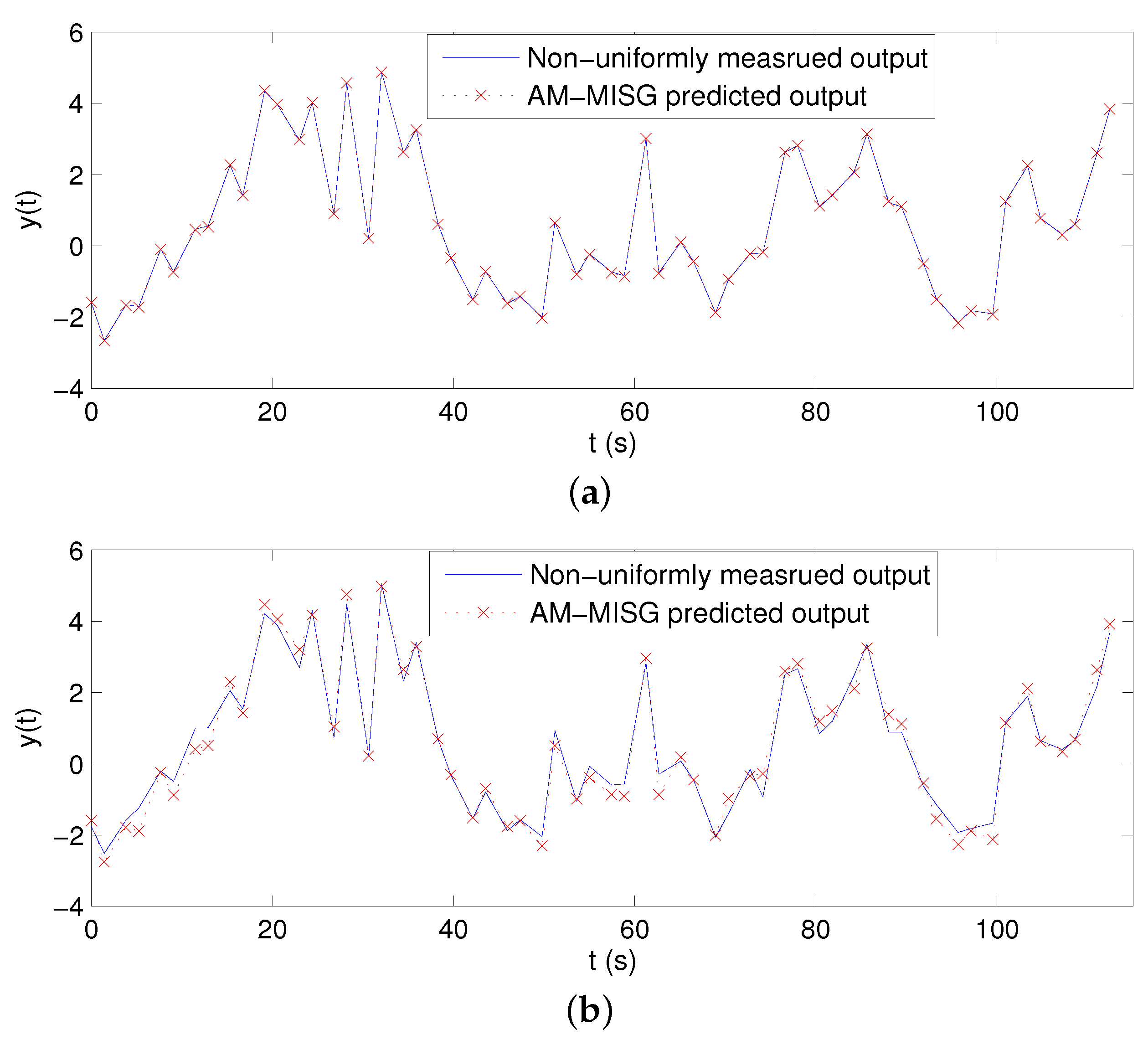
Considering the noise variance and , a separate dataset with length 30 has been generated for model validation, respectively. Using the mean values of the parameter estimates listed in Table 4 and Table 5 for to predict the outputs of the periodically non-uniformly sampled-data Hammerstein system, the results are shown in Figure 4, where the solid line and the x-marks represent the true measured outputs and the model predicted outputs, respectively. From Figure 4, it is clear that the model predictions can catch the trend of the true outputs well, and the prediction performance becomes better if a noise with smaller variance is introduced.
5. Conclusions
Based on the non-uniform input-output dataset, an auxiliary model-based stochastic gradient (AM-SG) algorithm is developed in this paper to estimate the parameters of Hammerstein systems. To improve the identification performance of the AM-SG algorithm, an auxiliary model-based multi-innovation stochastic gradient (AM-MISG) algorithm is proposed by introducing an innovation length p. The simulation results illustrate that the AM-MISG algorithm with a larger p can provide more accurate parameter estimates and a faster convergence rate. In addition, the proposed algorithm can be extended to identify more complex nonlinear systems with non-uniform sampling.
Acknowledgments
This paper is supported by the National Natural Science Foundation of China (No. 61403166), the Natural Science Foundation of Jiangsu Province (China; BK20140164) and Fundamental Research Funds for the Central Universities (JUSRP11561, JUSRP51510).
Author Contributions
Li Xie derived the identification algorithm and was in charge of the overall research. Huizhong Yang helped with preparing the manuscript.
Conflicts of Interest
The authors declare no conflict of interest.
References
- Liu, Y.; Wang, H.; Yu, J.; Li, P. Selective recursive kernel learning for online identification of nonlinear systems with NARX form. J. Process Control 2010, 20, 181–194. [Google Scholar] [CrossRef]
- Tang, Y.; Li, Z.; Guan, X. Identification of nonlinear system using extreme learning machine based Hammerstein model. Commun. Nonlinear Sci. Numer. Simul. 2014, 19, 3171–3183. [Google Scholar] [CrossRef]
- Giri, F.; Bai, E.W. Block-Oriented Nonlinear System Identification; Springer: London, UK, 2010. [Google Scholar]
- Wills, A.; Schön, T.B.; Ljung, L.; Ninness, B. Identification of Hammerstein-Wiener models. Automatica 2013, 49, 70–81. [Google Scholar] [CrossRef]
- Lawrynczuk, M. Nonlinear predictive control for Hammerstein-Wiener systems. ISA Trans. 2014, 55, 49–62. [Google Scholar] [CrossRef] [PubMed]
- Wang, Y.Y.; Wang, X.D.; Wang, D.Q. Identification of dual-rate sampled Hammerstein systems with a piecewise-linear nonlinearity using the key variable separation technique. Algorithms 2015, 8, 366–379. [Google Scholar] [CrossRef]
- Chen, J.; Wang, X.; Ding, R. Gradient based estimation algorithm for Hammerstein systems with saturation and dead-zone nonlinearities. Appl. Math. Model. 2012, 36, 238–243. [Google Scholar] [CrossRef]
- Lv, X.; Ren, X. Non-iterative identification and model following control of Hammerstein systems with asymmetric dead-zone non-linearities. IET Control Theory Appl. 2012, 6, 84–89. [Google Scholar] [CrossRef]
- Giri, F.; Rochdi, Y.; Brouri, A.; Chaoui, F.Z. Parameter identification of Hammerstein systems containing backlash operators with arbitrary-shape parametric borders. Automatica 2011, 47, 1827–1833. [Google Scholar] [CrossRef]
- Fang, L.; Wang, J.; Zhang, Q. Identification of extended Hammerstein systems with hysteresis-type input nonlinearities described by Preisach model. Nonlinear Dyn. 2015, 79, 1257–1273. [Google Scholar] [CrossRef]
- Zhang, Q.; Wang, Q.; Li, G. Nonlinear modeling and predictive functional control of Hammerstein system with application to the turntable servo system. Mech. Syst. Signal Process. 2016, 72, 383–394. [Google Scholar] [CrossRef]
- Pouliquen, M.; Pigeon, E.; Gehan, O. Identification scheme for Hammerstein output error models with bounded noise. IEEE Trans. Autom. Control 2016, 61, 550–555. [Google Scholar] [CrossRef]
- Ding, F.; Shi, Y.; Chen, T. Auxiliary model-based least-squares identification methods for Hammerstein output-error systems. Syst. Control Lett. 2007, 56, 373–380. [Google Scholar] [CrossRef]
- Filipovic, V.Z. Consistency of the robust recursive Hammerstein model identification algorithm. J. Frankl. Inst. 2015, 352, 1932–1945. [Google Scholar] [CrossRef]
- Gao, X.; Ren, X.; Zhu, C.; Zhang, C. Identification and control for Hammerstein systems with hysteresis non-linearity. IET Control Theory Appl. 2015, 9, 1935–1947. [Google Scholar] [CrossRef]
- Cao, P.; Luo, X. Performance analysis of multi-innovation stochastic Newton recursive algorithms. Digit. Signal Process. 2016, 56, 15–23. [Google Scholar] [CrossRef]
- Ding, F. Complexity, convergence and computational efficiency for system identification algorithms. Control Decis. 2016, 31, 1729–1741. [Google Scholar]
- Ding, F. Several multi-innovation identification methods. Digit. Signal Process. 2010, 20, 1027–1039. [Google Scholar] [CrossRef]
- Shi, Z.; Wang, Y.; Ji, Z. A multi-innovation recursive least squares algorithm with a forgetting factor for Hammerstein CAR systems with backlash. Circuits Syst. Signal Process. 2016, 35, 4271–4289. [Google Scholar] [CrossRef]
- Xiao, Y.; Song, G.; Liao, Y.; Ding, R. Multi-innovation stochastic gradient parameter estimation for input nonlinear controlled autoregressive models. Int. J. Control Autom. Syst. 2012, 10, 639–643. [Google Scholar] [CrossRef]
- Chen, J.; Zhang, Y.; Ding, R. Gradient-based parameter estimation for input nonlinear systems with ARMA noises based on the auxiliary model. Nonlinear Dyn. 2013, 72, 865–871. [Google Scholar] [CrossRef]
- Ma, J.; Xiong, W.; Ding, F.; Alsaedi, A.; Hayat, T. Data filtering based forgetting factor stochastic gradient algorithm for Hammerstein systems with saturation and preload nonlinearities. J. Frankl. Inst. 2016, 353, 4280–4299. [Google Scholar] [CrossRef]
- Li, W.; Shah, S.L.; Xiao, D. Kalman filters in non-uniformly sampled multirate systems: For FDI and beyond. Automatica 2008, 44, 199–208. [Google Scholar] [CrossRef]
- Albertos, P.; Salt, J. Non-uniform sampled-data control of MIMO systems. Ann. Rev. Control 2011, 35, 65–76. [Google Scholar] [CrossRef]
- Ding, F.; Wang, F.F. Recursive least squares identification algorithms for linear-in-parameter systems with missing data. Control Decis. 2016, 31, 2261–2266. [Google Scholar]
- Yang, H.; Xia, Y.; Shi, P. Stabilization of networked control systems with nonuniform random sampling periods. Int. J. Robust Nonlinear Control 2011, 21, 501–526. [Google Scholar] [CrossRef]
- Aibing, Q.; Bin, J.; Chenglin, W.; Zehui, M. Fault estimation and accommodation for networked control systems with nonuniform sampling periods. Int. J. Adapt. Control Signal Process. 2015, 29, 427–442. [Google Scholar] [CrossRef]
- Sheng, J.; Chen, T.; Shah, S.L. Generalized predictive control for non-uniformly sampled systems. J. Process Control 2002, 12, 875–885. [Google Scholar] [CrossRef]
- Khan, S.; Goodall, R.; Dixon, R. Non-uniform sampling strategies for digital control. Int. J. Syst. Sci. 2013, 44, 2234–2254. [Google Scholar] [CrossRef]
- Jing, S.; Pan, T.; Li, Z. Recursive bayesian algorithm with covariance resetting for identification of Box-Jenkins systems with non-uniformly sampled input data. Circuits Syst. Signal Process. 2016, 35, 919–932. [Google Scholar] [CrossRef]
- Xie, L.; Yang, H.; Ding, F. Identification of non-uniformly sampled-data systems with asynchronous input and output data. J. Frankl. Inst. 2017, 354, 1974–1991. [Google Scholar] [CrossRef]
- Li, X.; Ding, R.; Zhou, L. Least-squares-based iterative identification algorithm for Hammerstein nonlinear systems with non-uniform sampling. Int. J. Comput. Math. 2013, 90, 1524–1534. [Google Scholar] [CrossRef]
- Salt, J.; Albertos, P. Model-based multirate controllers design. IEEE Trans. Control Syst. Technol. 2005, 13, 988–997. [Google Scholar] [CrossRef]
- Huang, J.; Shi, Y.; Huang, H.; Li, Z. l2-l∞ filtering for multirate nonlinear sampled-data systems using T-S fuzzy models. Digit. Signal Process. 2013, 23, 418–426. [Google Scholar] [CrossRef]
- Xie, L.; Yang, H.; Ding, F.; Huang, B. Novel model of non-uniformly sampled-data systems based on a time-varying backward shift operator. J. Process Control 2016, 43, 38–52. [Google Scholar] [CrossRef]
- Chang, F.; Luus, R. A noniterative method for identification using Hammerstein model. IEEE Trans. Autom. Control 1971, 16, 464–468. [Google Scholar] [CrossRef]
- Shen, Q.; Ding, F. Least squares identification for Hammerstein multi-input multi-output systems based on the key-term separation technique. Circuits Syst. Signal Process. 2016, 35, 1–14. [Google Scholar] [CrossRef]
- Zhang, Y.; Zhao, Z.; Cui, G. Auxiliary model method for transfer function estimation from noisy input and output data. Appl. Math. Model. 2014, 39, 4257–4265. [Google Scholar] [CrossRef]
- Jin, Q.; Wang, Z.; Liu, X. Auxiliary model-based interval-varying multi-innovation least squares identification for multivariable OE-like systems with scarce measurements. J. Process Control 2015, 35, 154–168. [Google Scholar] [CrossRef]
- Ding, J. Data filtering based recursive and iterative least squares algorithms for parameter estimation of multi-input output systems. Algorithms 2016, 9, 49. [Google Scholar] [CrossRef]
- Bai, E.W. An optimal two-stage identification algorithm for Hammerstein-Wiener nonlinear systems. Automatica 1998, 34, 333–338. [Google Scholar] [CrossRef]
- Wang, X.; Ding, F. Convergence of the auxiliary model-based multi-innovation generalized extended stochastic gradient algorithm for Box-Jenkins systems. Nonlinear Dyn. 2015, 82, 269–280. [Google Scholar] [CrossRef]
Figure 1.
Periodically non-uniformly sampled-data Hammerstein system.
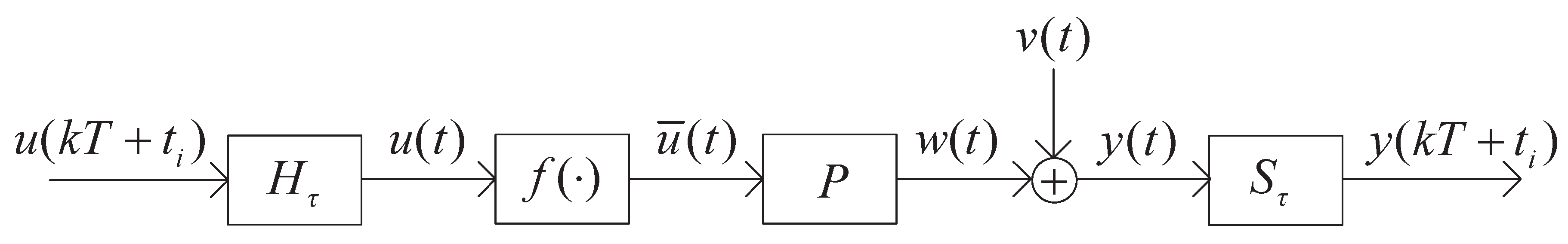
Figure 2.
The flowchart of computing the parameter estimate.
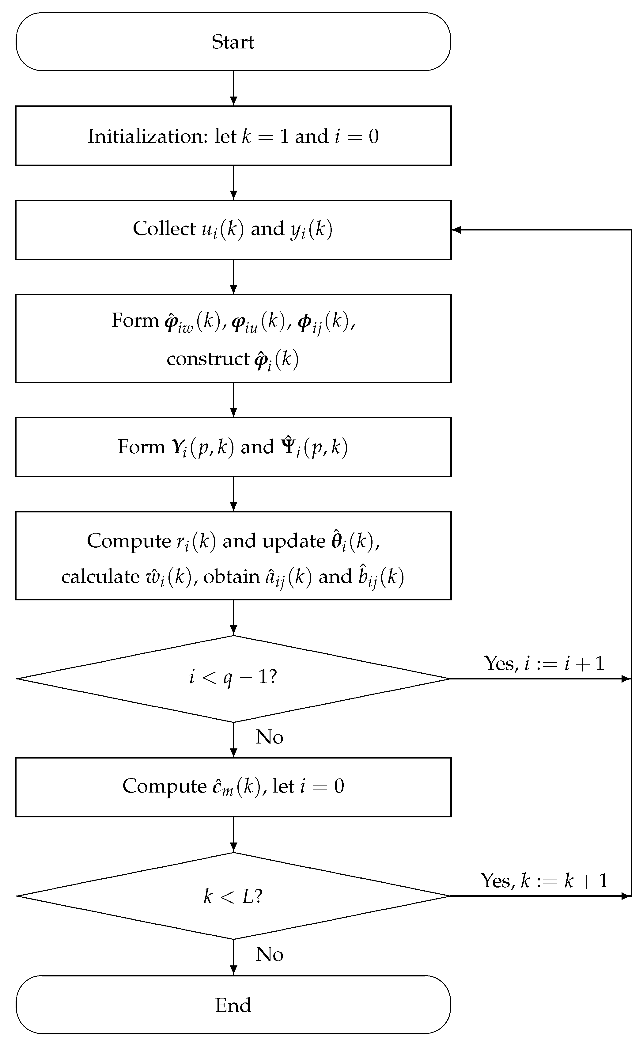
Figure 3.
The AM-MISG estimation errors versus k with , 5, 12.
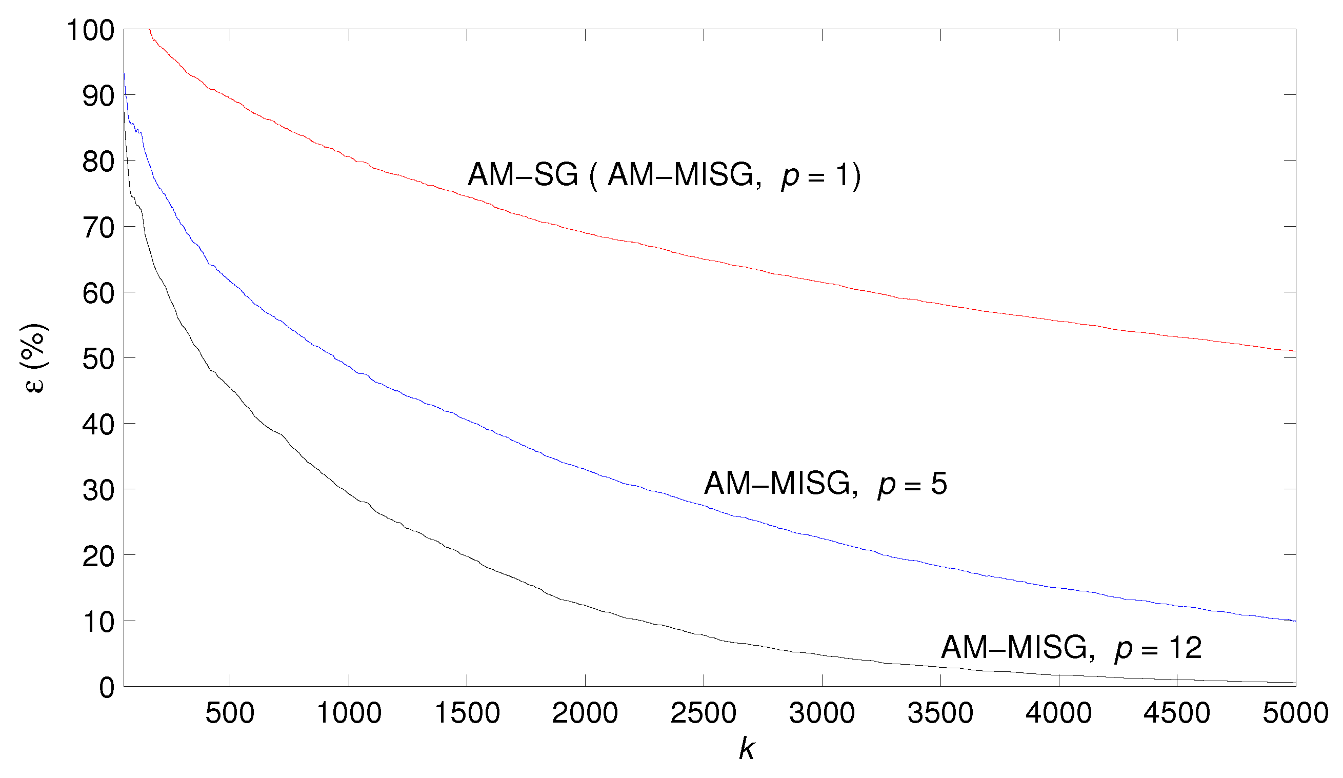
Figure 4.
The predicted outputs and the measured outputs. (a) For the noise variance . (b) For the noise variance .
Figure 4.
The predicted outputs and the measured outputs. (a) For the noise variance . (b) For the noise variance .

Table 1.
The auxiliary model-based multi-innovation stochastic gradient (AM-MISG) parameter estimates and errors ().
Table 1.
The auxiliary model-based multi-innovation stochastic gradient (AM-MISG) parameter estimates and errors ().
| k | 100 | 200 | 500 | 1000 | 2000 | 3000 | 4000 | 5000 | True Values |
|---|---|---|---|---|---|---|---|---|---|
| −0.23798 | −0.23467 | −0.24155 | −0.23676 | −0.32003 | −0.37711 | −0.42344 | −0.46120 | −0.80860 | |
| −0.17253 | −0.15925 | −0.14095 | −0.10136 | −0.07608 | −0.04580 | −0.00265 | 0.02211 | 0.25514 | |
| 0.21247 | 0.28325 | 0.36820 | 0.43435 | 0.54777 | 0.63347 | 0.70653 | 0.76997 | 1.00000 | |
| 0.03019 | 0.01933 | 0.01196 | 0.00916 | 0.00769 | −0.01410 | −0.04420 | −0.08780 | −0.61623 | |
| 0.08793 | 0.10742 | 0.14003 | 0.18442 | 0.23272 | 0.28553 | 0.31263 | 0.32151 | 0.50931 | |
| −0.14144 | −0.17751 | −0.20109 | −0.25406 | −0.32583 | −0.39976 | −0.44355 | −0.49299 | −0.94779 | |
| −0.26469 | −0.24184 | −0.17359 | −0.12188 | −0.07576 | −0.02374 | 0.04034 | 0.07391 | 0.57794 | |
| 0.24088 | 0.32232 | 0.39463 | 0.45898 | 0.57929 | 0.66877 | 0.73108 | 0.77370 | 1.00000 | |
| 0.02779 | 0.05257 | 0.07272 | 0.09047 | 0.11098 | 0.11615 | 0.10811 | 0.09453 | −0.49522 | |
| 0.04644 | 0.04343 | 0.04713 | 0.07480 | 0.12538 | 0.16100 | 0.18916 | 0.22188 | 0.75553 | |
| 1.05391 | 0.96668 | 0.98187 | 0.93895 | 0.80087 | 0.72297 | 0.66712 | 0.63075 | 0.50000 | |
| 1.79633 | 1.68065 | 1.44046 | 1.16009 | 0.82335 | 0.65456 | 0.52589 | 0.45922 | 0.25000 | |
| 103.04890 | 97.41924 | 89.40996 | 80.57154 | 68.94369 | 61.44114 | 55.52206 | 51.00555 |
Table 2.
The AM-MISG parameter estimates and errors ().
| k | 100 | 200 | 500 | 1000 | 2000 | 3000 | 4000 | 5000 | True Values |
|---|---|---|---|---|---|---|---|---|---|
| −0.17179 | −0.18574 | −0.31748 | −0.41405 | −0.61777 | −0.71905 | −0.76959 | −0.80135 | −0.80860 | |
| −0.17111 | −0.11012 | −0.05496 | 0.01077 | 0.12643 | 0.17775 | 0.21975 | 0.24397 | 0.25514 | |
| 0.37344 | 0.45616 | 0.62647 | 0.76016 | 0.91687 | 0.95693 | 0.98483 | 0.99692 | 1.00000 | |
| 0.06673 | 0.04317 | 0.02695 | −0.05431 | −0.24467 | −0.39466 | −0.50874 | −0.56748 | −0.61623 | |
| 0.18052 | 0.22395 | 0.27192 | 0.33856 | 0.35650 | 0.39392 | 0.41745 | 0.43668 | 0.50931 | |
| −0.34108 | −0.41100 | −0.47313 | −0.56512 | −0.68070 | −0.77319 | −0.82088 | −0.85964 | −0.94779 | |
| −0.01887 | −0.03044 | 0.07773 | 0.16053 | 0.30682 | 0.37436 | 0.44459 | 0.47782 | 0.57794 | |
| 0.38009 | 0.49836 | 0.59120 | 0.75693 | 0.92872 | 0.97376 | 0.98098 | 0.98525 | 1.00000 | |
| 0.02215 | 0.04295 | 0.06078 | 0.02968 | −0.07356 | −0.20574 | −0.29673 | −0.36568 | −0.49522 | |
| 0.10985 | 0.13310 | 0.18300 | 0.25133 | 0.33733 | 0.43426 | 0.52067 | 0.59753 | 0.75553 | |
| 0.97825 | 0.90595 | 0.80559 | 0.63455 | 0.51789 | 0.50729 | 0.50178 | 0.50388 | 0.50000 | |
| 1.35667 | 1.13733 | 0.73326 | 0.47388 | 0.31951 | 0.27787 | 0.26181 | 0.25438 | 0.25000 | |
| 84.52995 | 75.91772 | 61.64633 | 48.73054 | 32.94076 | 22.45332 | 15.03823 | 10.03271 |
Table 3.
The AM-MISG parameter estimates and errors ().
| k | 100 | 200 | 500 | 1000 | 2000 | 3000 | 4000 | 5000 | True Values |
|---|---|---|---|---|---|---|---|---|---|
| −0.21097 | −0.29207 | −0.48337 | −0.62718 | −0.78913 | −0.82242 | −0.82167 | −0.81394 | −0.80860 | |
| −0.09616 | −0.00999 | 0.04310 | 0.14720 | 0.23542 | 0.25631 | 0.25755 | 0.25552 | 0.25514 | |
| 0.46831 | 0.60206 | 0.82476 | 0.92527 | 0.99463 | 0.99562 | 0.99966 | 1.00088 | 1.00000 | |
| 0.05982 | 0.04225 | −0.06860 | −0.27395 | −0.53707 | −0.61472 | −0.62645 | −0.62093 | −0.61623 | |
| 0.27987 | 0.32848 | 0.34589 | 0.38704 | 0.42283 | 0.47864 | 0.49652 | 0.50327 | 0.50931 | |
| −0.42997 | −0.51235 | −0.60352 | −0.72537 | −0.84006 | −0.90571 | −0.93254 | −0.94364 | −0.94779 | |
| −0.00011 | 0.04270 | 0.21788 | 0.32975 | 0.47520 | 0.53405 | 0.56383 | 0.57217 | 0.57794 | |
| 0.44256 | 0.61696 | 0.76526 | 0.92836 | 1.00028 | 0.99858 | 0.99669 | 1.00004 | 1.00000 | |
| 0.01971 | 0.05871 | 0.01162 | −0.14602 | −0.33453 | −0.42806 | −0.46968 | −0.48801 | −0.49522 | |
| 0.11625 | 0.16567 | 0.24897 | 0.36557 | 0.55820 | 0.68047 | 0.73284 | 0.75125 | 0.75553 | |
| 0.88043 | 0.76552 | 0.64129 | 0.52932 | 0.49418 | 0.49855 | 0.50087 | 0.49915 | 0.50000 | |
| 1.04485 | 0.79819 | 0.45534 | 0.30318 | 0.25542 | 0.25328 | 0.25163 | 0.25057 | 0.25000 | |
| 73.56646 | 62.33004 | 45.43354 | 29.28325 | 12.29280 | 4.72652 | 1.75023 | 0.55900 |
Table 4.
The AM-MISG parameter estimates with standard deviations ().
| Parameters | True Values | |||
|---|---|---|---|---|
| −0.80860 | ||||
| 0.25514 | ||||
| 1.00000 | ||||
| −0.61623 | ||||
| 0.50931 | ||||
| −0.94779 | ||||
| 0.57794 | ||||
| 1.00000 | ||||
| −0.49522 | ||||
| 0.75553 | ||||
| 0.50000 | ||||
| 0.25000 |
Table 5.
The AM-MISG parameter estimates with standard deviations ().
| Parameters | True Values | |||
|---|---|---|---|---|
| −0.80860 | ||||
| 0.25514 | ||||
| 1.00000 | ||||
| −0.61623 | ||||
| 0.50931 | ||||
| −0.94779 | ||||
| 0.57794 | ||||
| 1.00000 | ||||
| −0.49522 | ||||
| 0.75553 | ||||
| 0.50000 | ||||
| 0.25000 |
© 2017 by the authors. Licensee MDPI, Basel, Switzerland. This article is an open access article distributed under the terms and conditions of the Creative Commons Attribution (CC BY) license (http://creativecommons.org/licenses/by/4.0/).
Share and Cite
MDPI and ACS Style
Xie, L.; Yang, H. Auxiliary Model Based Multi-Innovation Stochastic Gradient Identification Algorithm for Periodically Non-Uniformly Sampled-Data Hammerstein Systems. Algorithms 2017, 10, 84. https://doi.org/10.3390/a10030084
AMA Style
Xie L, Yang H. Auxiliary Model Based Multi-Innovation Stochastic Gradient Identification Algorithm for Periodically Non-Uniformly Sampled-Data Hammerstein Systems. Algorithms. 2017; 10(3):84. https://doi.org/10.3390/a10030084
Chicago/Turabian StyleXie, Li, and Huizhong Yang. 2017. "Auxiliary Model Based Multi-Innovation Stochastic Gradient Identification Algorithm for Periodically Non-Uniformly Sampled-Data Hammerstein Systems" Algorithms 10, no. 3: 84. https://doi.org/10.3390/a10030084
Note that from the first issue of 2016, this journal uses article numbers instead of page numbers. See further details here.