Properties of Vector Embeddings in Social Networks

Department of Computer Science and Mathematics, University of Passau, 94032 Passau, Germany
*
Author to whom correspondence should be addressed.
Algorithms 2017, 10(4), 109; https://doi.org/10.3390/a10040109
Submission received: 15 July 2017
/
Revised: 4 September 2017
/
Accepted: 11 September 2017
/
Published: 27 September 2017
(This article belongs to the Special Issue Algorithms in Online Social Networks)
Abstract
:Embedding social network data into a low-dimensional vector space has shown promising performance for many real-world applications, such as node classification, node clustering, link prediction and network visualization. However, the information contained in these vector embeddings remains abstract and hard to interpret. Methods for inspecting embeddings usually rely on visualization methods, which do not work on a larger scale and do not give concrete interpretations of vector embeddings in terms of preserved network properties (e.g., centrality or betweenness measures). In this paper, we study and investigate network properties preserved by recent random walk-based embedding procedures like node2vec, DeepWalk or LINE. We propose a method that applies learning to rank in order to relate embeddings to network centralities. We evaluate our approach with extensive experiments on real-world and artificial social networks. Experiments show that each embedding method learns different network properties. In addition, we show that our graph embeddings in combination with neural networks provide a computationally efficient way to approximate the Closeness Centrality measure in social networks.
1. Introduction
Social network analysis has been attracting great attention in the recent years. This is in part because social networks form an important class of networks that span a wide variety of media, ranging from social websites, such as Facebook, Twitter and citation networks of academic papers. Mining and analyzing data from these social network sites generated interesting insights, like, for example, insights on network formation processes (e.g., [1,2]), content distribution processes (e.g., [3,4]) and human (online) behavior (e.g., [5,6]). Furthermore, interesting applications have become possible, like, for example, different types of recommender systems [7,8] or media analysis applications [9].
Data Analysis and Machine Learning techniques play an essential role in mining social network data. However, whenever we use such statistical machine learning techniques on graph analysis tasks, we have to find a suitable vectorial representation for a network at hand. The most straightforward representation consists of an adjacency matrix, where edges between nodes are indicated as an entry in a squared matrix. Due to its quadratic size and its sparsity the adjacency matrix is not very well suited for traditional machine learning algorithms. As a remedy, low-dimensional vector embeddings have become a promising and powerful tool for analyzing large social networks.
Graph embeddings represent every node in a graph as a low-dimensional, real-valued vector preserving different network properties, like, for example, first- or second-order proximities [10] or topological-structures [11]. Typically, graph embeddings have been obtained by computationally intensive eigenvalue decomposition methods. Motivated by the success of deep learning techniques in the natural language processing (NLP) area, several novel graph embedding methods have been proposed. They learn dense vector representations utilizing random walks over the network. For example, DeepWalk [12] samples node sequences and feeds them to a Skip-Gram based of Word2Vec [13] model to train node representations. LINE [14] optimizes the objective function to preserve both the local and the global network structures. In extension to these methods, Node2vec [10] introduces mechanisms to balance the random walk between Breadth-First Search (BFS) sampling and Depth-First Search (DFS) sampling, thereby allowing to preserve more local or global structures. In [15], authors exploit an extension of the Word2Vec algorithm, the Paragraph Vector [16], to learn embeddings for local regions of the network. These local regions are defined as neighborhoods around a focal node, as it is usually seen in ego-networks [17].
Overall, graph embeddings have shown promising performance for various graph analytic tasks such as node classification [17], clustering [18], link prediction [19], knowledge extraction from semantic networks [20] and network visualization [21]. However, due to the stochastic nature of the random walk, it remains unclear what graph properties are retained exactly in a given set of embeddings. Understanding the rather abstract vectorial representation of a node embedding can be compared to the effort in understanding the structure of neural networks in image processing. One possible solution in the field of image processing, therefore, is to reconstruct exemplary images from particularly activated parts of the neural network [22]. Since neural networks are usually organized into different layers detecting features of different granularity, we can find the (usually abstract) input image that maximizes a neuron of a layer. Hence, the role of a particular element in the neural network can be described in terms of input that maximizes its activation.
A similar idea would be quite helpful for graph embeddings when one wants to know the parts of the social network, i.e., the input space for our network-embedding problem, which are preserved. Hence, the abstract vectorial representation of a node can be mapped back in input space to understand the properties observed by the representation. However, to the best of our knowledge, there is no method and corresponding study which investigates how to analyze graph properties preserved by random-walk based graph embeddings. Moreover, when certain graph properties are retained in the vector embeddings, we can try to reconstruct those properties given the embeddings alone. Since random-walk based graph embeddings can be computed in linear time [10], finding a way to reconstruct graph measures from those embeddings with a high computational complexity, like, for example, closeness or betweenness centrality [24], could allow us to find computationally efficient approximations.
Given this motivation, we make the following contributions in our work:
Contribution 1: We propose a new methodology to identify graph properties preserved by random-walk based graph embedding methods (Section 4). In particular, we are interested in graph properties explaining the similarity of the local neighborhood of a node. In addition, two nodes are accounted to be similar if they show similar graph characteristics in their local neighborhood, like, for example, similar topological structures (e.g., same degree) or comparable centrality and betweenness distributions. Therefore, we propose to relate the neighborhood-similarity between two nodes to the similarity of the embeddings by solving a learning to rank problem. Hence, the network measure with the highest contribution to the similarity of two nodes can be considered as the highest explanatory factor regarding their relatedness in embedding space. The results show that random-walk based embedding techniques can be grouped into two categories, depending on the properties of the random walk. LINE and DeepWalk walk globally over the graph and thus learn betweenness and eigenvector centrality. Node2vec and our Paragraph Vector method retain local properties such as degree centrality.
Contribution 2: We examine whether embeddings can be used to predict centrality values directly (Section 4). We apply neural networks to a regression task which attempts to approximate centrality values using embeddings as input. In particular, we utilize a multi-layer feed-forward neural network to approximate the centrality of a node given its embedding. We show that, specifically, closeness centrality can be approximated best compared to other centralities by our method. In particular, generating embeddings and training the neural network can be computed in approximately linear time [12,25] (but with a high overhead). Therefore, our results suggest that closeness centrality can be approximated efficiently in linear time. However, we do not give a formal proof of the runtime complexity computation as it goes beyond the current study.
The remainder of the paper is organized as follows. In Section 2, we provide the definitions required to understand the problem and models. In Section 3, we provide a short overview on recent embedding techniques and inspecting approaches. In Section 4, we define the problem that we want to study and the proposed method. In Section 5, we then describe our experimental setup and evaluate the proposed approach. Finally, in Section 6, we draw our conclusions and discuss future research directions.
2. Definitions and Preliminaries
A graph consists of a set of n nodes and a set of edges between nodes. The adjacency matrix of G is the -matrix A with entries
We restrict ourselves to undirected graphs, where, for all nodes , we have if and only if —or, equivalently, where the adjacency matrix is symmetric. For a node , the ego-network of u is the restriction of G to u and all its neighbors. We denote the set of egos in a social graph by .
Definition 1
(Graph embedding). Let G be a graph. An embedding of G is a map , where . Therefore, denotes the embeddings of the graph G and the ith row of Y.
Definition 2
(First-order Proximity). The first-order proximity in a graph is the local pairwise proximity between two nodes. For each pair of nodes linked by an edge , the weight on that edge, , indicates the first-order proximity between and . If no edge is observed between and , their first-order proximity is 0.
Definition 3
(Second-order Proximity). The second-order proximity between a pair of vertexes describes the proximity of the pair’s neighborhood structure. Let denote the first-order proximity between and other vertexes. Then, second-order proximity is determined by the similarity of and . Second-order proximity compares the neighborhood of two nodes and treats them as similar if they have a similar neighborhood.
3. Related Work
3.1. Graph Embedding Techniques
Recently, methods that use distributed representation learning techniques in an NLP domain, like the Skip-Gram algorithm, have gained attention from the research community. These NLP methods have been adapted to calculate graph embeddings that preserve first and second order proximities. For obtaining the embeddings, these methods create symbolic sequences comparable to natural language text by conducting random-walks over the graph. The methods yield lower time complexity compared to eigenvalue decomposition methods [26]. Moreover, they are able to map the nonlinear structure of the network into the embedding space. They are especially useful when one can either only partially observe the graph, or the graph is too large. In this section, we quickly review the different random-walk based embedding techniques:
- DeepWalk [12]: This approach learns d-dimensional feature representations by simulating uniform random walks over the graph. It preserves higher-order proximities by maximizing the probability of observing the last c nodes and the next c nodes in the random walk centered at . More formally, DeepWalk maximizes:where is the embedding vector of the node and c is the context size. We denote the mapping function for this method , where d is the embedding size. Therefore, the DeepWalk embedding of the node v is denoted by .
- node2vec [10]: Inspired by DeepWalk, node2vec preserves higher-order proximities by maximizing the probability of occurrence of subsequent nodes in fixed length random walks. The crucial difference from DeepWalk is that node2vec employs biased-random walks that provide a trade-off between BFS and DFS graph searches, and hence produces higher-quality and more informative embeddings than DeepWalk. More specifically, there are two key hyper-parameters and that control the random walk. Parameter p controls the likelihood of immediately revisiting a node in the walk. Parameter q controls the traverse behavior to approximate BFS or DFS. For , node2vec is identical to DeepWalk. We denote the node2vec embedding by node2vec: , where d is the embedding size. Therefore, the node2vec embedding of the node v is shown by node2vec.
- loc [15]: This approach limits random walks to the neighborhood around egos to make artificial paragraphs. ParagraphVector [16] is properly applied to learn local embeddings for egos by optimizing the likelihood objective using stochastic gradient descent with negative sampling [27]. Formally, given an artificial paragraph for ego , the goal is to update representations in order to maximize the average log probability:where is the embedding vector of the ego , l is the length of the artificial paragraph, and c is the context size. Therefore, there is a mapping function , where d is the embedding size. We denote the loc embedding of the ego u by .
- LINE [14]: It learns two embedding vectors for each node by preserving the first-order and second-order proximity of the network in two phases. In the first phase, it learns dimensions by BFS-style simulations over immediate neighbors of nodes. In the second phase, it learns the next dimensions by sampling nodes strictly at a 2-hop distance from the source nodes. Then, the embedding vectors are concatenated as the final representation for a node. Indeed, LINE defines two joint probability distributions for each pair of nodes, one using adjacency matrix and the other using the embedding. It minimizes the Kullback–Leibler (KL) divergence [28] of these two distributions. The first phase distributions and the objective function are as follows:Probability distributions and objective function are similarly defined for the second phase. This technique adopts the asynchronous stochastic gradient algorithm (ASGD) [29] for optimization. In each step, the ASGD algorithm samples a mini-batch of nodes and then updates the model parameters. We denote this embedding as a function that maps nodes to the vector space, where d is the embedding size. Therefore, the LINE embedding of the node v is denoted by .
3.2. Techniques for Inspecting Embeddings
Graph embeddings usually create vectors of several 100 dimensions per node in the graph. While eigenvalue based decomposition methods give some formal guarantees on the retained network properties, random-walk based methods are stochastic in nature and depend heavily on hyper-parameter settings. Therefore, analyzing the retained graph properties requires either applying the embeddings to particular graph analysis tasks, like node classification, clustering, community detection or link prediction, or to visualize structural relationships. For example, if two nodes u and v are directly connected in the graph, they should appear close to each other when in a visualized embedding space. In this section, we review different methods to inspect graph embeddings in order to motivate the development of our own approach.
- Visualization: To gain insight into binary relationships between objects, the relations are often coded into a graph, which is then visualized. The visualization is usually split in the layout and the drawing phase. The layout is a mapping of graph elements to points in . The drawing assigns graphical shapes to the graph elements and draws them using the positions computed in the layout [30]. The effectiveness of DeepWalk is illustrated by visualizing the Zachary’s Karate Club network [12]. The authors of LINE visualized the DataBase systems and Logic Programming (DBLP) co-authorship network, and showed that LINE is able to cluster together authors in the same field. Structural Deep Network Embedding (SDNE) [31] was applied on a 20-Newsgroup document similarity network to obtain clusters of documents based on topics.
- Network Compression: The idea in network compression is to reconstruct the graph with a smaller number of edges [23]. Graph embedding can also be interpreted as a compression of the graph. Wang et al. [31] and Ou et al. [32] tested this hypothesis explicitly by reconstructing the original graph from the embedding and evaluating the reconstruction error. They show that a low-dimensional representation for each node suffices to reconstruct the graph with high precision.
- Classification: Often in social networks, a fraction of nodes are labeled which indicate interests, beliefs, or demographics, but the rest are missing labels. Missing labels can be inferred using the labeled nodes through links in the network. The task of predicting these missing labels is also known as node classification. Recent work [10,12,14,31] has evaluated the predictive power of embedding on various information networks including language, social, biology and collaboration graphs. The authors in [15] predict the social circles for a new node added into the network.
- Clustering: Graph clustering in social networks aim to detect social communities. In [33], the authors evaluated the effectiveness of embedding representations of DeepWalk and LINE on network clustering. Both approaches showed nearly the same performance.
- Link Prediction: Social networks are constructed from the observed interactions between entities, which may be incomplete or inaccurate. The challenge often lies in predicting missing interactions. Link prediction refers to the task of predicting either missing interactions or links that may appear in the future in an evolving network. Link prediction is used to predict probable friendships, which can be used for recommendation and lead to a more satisfactory user experience. Liao et al. [34] used link prediction to evaluate node2vec and LINE. Node2vec outperforms LINE in terms of area under the Receiver Operating Characteristic (ROC) curve.
4. Approach
4.1. Problem Statement
Problem 1—Explaining Embedding Relatedness: Let G be a social network graph where every node has an embedding obtained from random-walk based embedding methods such as , , , and . The inner-product of two nodes u and v determines a similarity relation between the two nodes. Due to the random-walk based creation of the embeddings, we assume that this similarity can be approximated by similar network properties of the neighborhoods and of node u and v, respectively. Therefore, we aim to explain the inner-product by a weighted linear combination of centrality measures obtained from the neighborhoods and . Degree centrality , closeness centrality , betweenness centrality and eigenvector centrality have been chosen as centrality measures due to their importance in social network analysis and due to their well understood properties [35].
Closeness centrality of a node is the average sum of the inverse of the distance to other nodes. Formally, closeness is defined as:
where is the length of the shortest path between [36].
Betweenness centrality counts the fraction of shortest paths going through a node. Betweenness centrality of a node u is then formally defined as follows:
where is the number of shortest paths between node and that pass through node u. is the number of shortest paths between node and [36].
Eigenvector centrality generalizes degree centrality by incorporating the importance of the neighbors. The eigenvector centrality of is a function of its neighbors’ centralities. It is proportional to the summation of their centralities:
where is some fixed constant [36].
Closeness centrality is widely used to study information flow in social networks [37]. Betweenness and eigenvector centrality are commonly used to detect and investigate community structure in social networks [38].
Problem 2—Predicting network properties: In order to consider single nodes without a neighborhood, we consider the problem of predicting the centrality values , , and for a particular node v based on its embeddings only. We aim to find a nonlinear mapping between the embedding vector and a single centrality property of its node. By obtaining such an approximately correct mapping, we can conclude that the vector space of the embeddings retains the structural information of the network property.
Overall, both case studies allow us to gain insights on the embedding properties in terms of centrality measures retained and the relatedness of their neighborhoods. In addition, predicting network properties successfully allows us to approximate computationally complex centrality measures more efficiently.
4.2. Explaining Embedding Relatedness
We formulate our approach such that the similarity of two embeddings and can be approximated by a weighted sum of network properties:
where is a function that computes similarity of the pair based on network property i, k is the number of network properties considered, and is the weight of the network property i. To estimate the weights for every property, we cast the problem into a learning to rank problem.
Learning to rank is an important problem in web page ranking, information retrieval and many other applications [39]. Given a ranking of items according to some query items, learning to rank obtains a function based on the similarity between the query and its ranked items. Several types of machine learning algorithms have been considered for this problem: pointwise methods, pairwise methods, and listwise methods. Most recent works have applied pairwise methods for learning to rank on graphs [40,41]. In pairwise ranking, one is given examples of order relationships among objects, and the goal is to learn from these examples, a real-valued ranking function that induces a ranking or ordering over the object space. We consider the problem of learning such a ranking function when the data is represented as a graph, in which nodes correspond to objects and embeddings encode similarities between objects. Among existing approaches for learning to rank, rankSVM [42] is a commonly used method extended from the popular support vector machine (SVM) [43] for data classification. In training an SVM classifier, a weight vector is computed on the training data. This weight vector can be used as an important measure of the centrality to the classifier. These weights can explain what combination of centralities can explain embeddings.
In learning to rank, we first sort nodes according to their similarities. More formally, for each node , we sort all other nodes according to the inner product similarity . Therefore, each pair of nodes has a rank label that we use as ground truth. We denote the ground-truth vector by , .
Furthermore, we need to compute the similarity in terms of DC, CC, BC and EC between every pair of nodes . Given a node , we calculate the centrality measures for every node , where defines the neighborhood of node . Indeed, in our approach, we consider network properties within a subgraph around a focal node. To compare how properties of two subgraphs are similar, we first calculate the probability distribution of each centrality by histogramming the centrality measures for every node . We then measure the similarity between two distributions over the same centrality by KL divergence as follows:
where and are probability distributions over the same centrality measure. If is low, it means the distributions are very similar and vice versa. In order to guarantee a certain stability of our approach, we assume that the KL divergence can be estimated in a reasonably large neighborhood and that the graph is connected.
Therefore, for each pair of nodes, we have a feature vector . We denote the feature matrix by . The rankSVM [42] model is built by minimizing the objective function
is the centrality vector, where denotes the weight for degree, is the weight for closeness, denotes the weight for betweenness, and is the weight for eigenvector centrality. is the regularization parameter. The C parameter provides a trade-off between the misclassification of training examples and the simplicity of the decision surface. A low parameter value makes the decision surface smooth, whereas a high parameter-value aims at classifying all training examples correctly by giving the model freedom to select more samples as support vectors. ℓ is a suitable loss function such as . is the regularization term to avoid overfitting by penalizing large coefficients in the solution vector [42]. The overall goal is to find w that optimizes the approximation of to t.
4.3. Predicting Graph Properties
In our second approach, we aim to analyze embedding properties in terms of single node properties. We formulate the problem as a regression task that attempts to predict centrality values using embeddings as input. In detail, we use a feed-forward neural network model for learning nonlinear relationships between the embedding as a input variables and the different centrality measures as single output variable [44]. The architecture of the model that approximates centrality values of is described as follows:
- Input layer: The input is given by one of the different embeddings for a single node, namely , , or .
- Hidden layer: The hidden layer consists of a single dense layer with ReLU activation units [45] .
- Output layer: The output layer has a sigmoid unit [46]. We choose the sigmoid unit since normalized centrality values are in the range of .
- Optimizer: Stochastic gradient descent (SGD) [47], which is a popular technique for large-scale optimization problems in machine learning.
Since centralities are continuous variables, we need an error criterion that measures, in a probabilistic sense, the error between the desired quantity and our estimate of it. Therefore, we use the mean squared error (MSE), which is a common measure of estimator quality of the fitted values of a dependent variable.
5. Experiments
In this section, we report on the conducted experiments to evaluate the effectiveness and efficiency of our proposed method. We apply the method to several real-world as well as artificial social networks. We consider normalized values of centralities in our experiments.
5.1. Dataset
Since our learning-to-rank method is based on estimating node similarities using distributional properties of their neighborhoods, we focus our experiments on data sets providing such structures. Ego-networks serve as possible datasets. In Ego-networks, every graph contains sub-graphs around a focal node called ego. The idea is to break up the large graph into smaller, easier to manage components and study the properties of the subgraphs. The ego-network model allows the small patterns, anomalies, and features to be discovered that would be missed when an entire graph is analyzed [15]. Therefore, we use ego-networks from three major social networking sites: Facebook, Google+, and Twitter, available from the University of Stanford [17]. Table 1 describes the details of the datasets we used in our experiments.
Moreover, we generate an artificial scale-free graph utilizing the Barabási–Albert model [48]. The Barabási–Albert model is an algorithm generating random graphs using a preferential attachment process. The process starts with an initial graph of m nodes. One new node is added to the network at each time step . In more detail, the preferential attachment process works as follows:
- With a probability , this new node connects to m existing nodes uniformly at random.
- With a probability , this new node connects to m existing nodes with a probability proportional to the degree of node which it will be connected to.
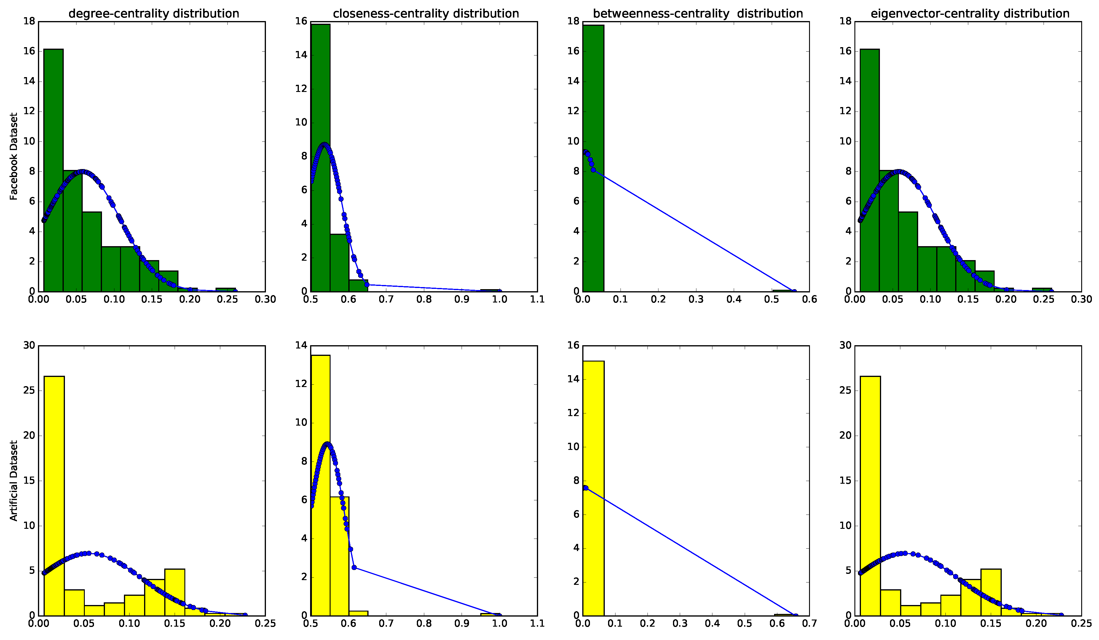
We simulate the Facebook graph using the Barabási–Albert model, which generates 87,516 edges for 4000 nodes. Similar to the Facebook dataset, we divide the Barabási–Albert graph into 10 ego-networks. The community library in Python [49] properly clusters the graph into several communities. We consider the node with highest betweenness as ego for each subgraph [17]. For further investigations, we compare degree, closeness, betweenness and eigenvector centrality distribution between one ego-network of the Facebook and one from the artificial graph. Figure 1 demonstrates centrality distribution of two random egos; ego ’686’ of the Facebook and ego ’25’ of the artificial dataset. We then require a metric to measure whether two distributions are identical. The Kolmogorov–Smirnov test [50] is the most popular test to find identical distributions. Therefore, we consider pairs of egos with similar size (number of edges) and use the Kolmogorov–Smirnov test. The Kolmogorov–Smirnov test generates two key values: KS statistic and p-value. If the KS statistic is small or the p-value is high, then the distributions of two samples are the same. Table 2 describes details for pairs of ego-networks that have nearly the same number of nodes. For all pairs, distributions are similar since KS statistic is low (around ) and the p-value is higher than [50].
5.2. Parameter Settings
- loc: Here, we apply Paragraph Vector [16] to learn embeddings for limited sequence of nodes, the same as paragraphs in text. In the Paragraph Vector Distributed Memory (PV-DM) model, optimal context size is 8 and the learned vector representations have 400 dimensions for both words and paragraphs [16].
- node2vec: This algorithm operates the same as DeepWalk, but the hyper-parameter p and q control the walking procedure. With the random walk is biased towards nodes close to the start node. Such walks obtain a local view of the underlying graph with respect to the start node in the walk and approximate BFS behavior in the sense that samples are comprised of nodes within a small locality. The parameter p controls the likelihood of immediately revisiting a node in the walk. If p is low , it would lead the walk to backtrack a step and this would keep the walk "local" close to the starting node. The optimal values of p and q depend a lot on the dataset [10]. In our experiment, we consider two settings: node2vec(1) keeps the walk local with , while node2vec(2) walks more exploratively with .
- LINE: LINE with first-order proximity, in which linked nodes will have closer representations, and LINE with second-order proximity, in which nodes with similar neighbors will have similar representations. In both settings, we consider the embedding size , batch-size= 1000, learning-rate .
5.3. Quantitative Results
In this section, we conduct two experiments: first, we inspect embeddings to see what network property is learned by each embedding technique. Second, we try to predict the centrality value itself.
5.3.1. Inspecting Embedding Properties
Embeddings as a low-dimensional representation of the graph are expected to preserve certain properties of the graph. Table 3 displays properties that are learned by rankSVM [42] using different embedding techniques. The following findings can be inferred from the table:
- Overall, we can explain the ranking either by combining betweenness or eigenvector or degree centralities of the node’s neighborhood. Closeness is not important in order to retain the ranking. The accuracy of SVM in all experiments is around , which shows that there are some explaining network properties missing.
- LINE and DeepWalk, which are able to explore the entire graph, can learn betweenness and eigenvector centrality of nodes. Betweenness is a global centrality metric that is based on shortest-path enumeration. Therefore, it is needed to walk over the whole graph to estimate betweenness centrality of nodes. Eigenvector centrality measures the influence of a node by exploiting the idea that connections to high-scoring nodes are more influential. This means that a node is important if it is connected to important neighbors. Therefore, computing eigenvector centrality also requires exploring globally the entire graph. This is done in practice by both LINE and DeepWalk, hence they learn eigenvector and betweenness centrality of nodes around .
- node2vec with and walks locally around the starting node. loc also walks over a limited area of the network. Therefore, they are not able to capture the structure of the entire network to learn betweenness or eigenvector centrality. The only property that is locally available is degree of nodes, hence is it learnt by node2vec(1) and loc.
- node2vec with and is more inclined to visit nodes that are further away from the starting node. Such behavior is reflective of DFS, which encourages outward exploration. Since node2vec(2) walks through the graph deeply, it could learn the eigenvector centrality.
5.3.2. Approximating Centrality Values
We aim to compute network centralities in an efficient time complexity. We report the results in terms of Mean Squared Error, hence smaller error gives better approximation. To approximate each centrality, we randomly selected of nodes in the Facebook graph as training set and the rest as a test. Table 4 demonstrates average value and standard deviation of centralities as well as errors where we feed the model with different embeddings. The Normalized Root Mean Squared Error (RMSE) is a standard statistical metric to measure model performance.
We also report results in terms of Normalized Root Mean Squared Error (NRMSE) and Coefficient of Variation of the RMSE:
where is the average of target values on test set. and are maximum and minimum of target values on test set [44].
It can be seen that, for closeness centrality, the error range is quite low compared to the average value, hence the regression model approximates closeness sufficiently well. Although closeness centrality has not been a relevant factor for explaining the ranking of nodes in our previous learning-to-rank experiment, a nonlinear mapping as provided by the neural network can estimate closeness values. A possible interpretation is the existence of local manifolds in embedding space containing nodes with similar closeness values. Since closeness represents the average distance of a node to all other nodes in the graph, it also hints that graph distances are preserved in embeddings space (in a nonlinear manner). However, for the other centrality measures, RMSE values are in the range of the average value or even higher. Hence, it seems that embeddings alone are not strong enough features to approximate these centralities.
6. Conclusions
This work has tackled graph embeddings to investigate network topological properties such as degree, closeness, betweenness, and eigenvector centrality. Empirical evaluation on real-world social networks indicated that each embedding technique can retain a different combination of network properties. We studied and reported recent existing methods of inspecting embeddings. We also presented an approach to approximate centrality values using neural networks. Our results revealed that closeness centrality is only centrality, and can be approximated in a more efficient time. For future work, we will analyze and compute the runtime of closeness centrality approximation precisely. We believe that there are some promising research directions exploiting embeddings to approximate some complex measures such as length of shortest path between two nodes.
Acknowledgments
This work is being supported by the German government in the BMBF-project ’Provenance Analytics’. The authors thank an anonymous colleague for proof-reading the mathematical equations and for his technical support while preparing the manuscript.
Author Contributions
The problem definition, theoretical analysis, and algorithm design were performed jointly by all authors; Michael Granitzer derived the theorems and Fatemeh Salehi Rizi implemented the algorithms depicted in the paper. All authors read and approved the final manuscript.
Conflicts of Interest
The authors declare no conflict of interest.
References
- Kossinets, G.; Watts, D.J. Empirical analysis of an evolving social network. Science 2006, 311, 88–90. [Google Scholar] [CrossRef] [PubMed]
- Romero, D.M.; Kleinberg, J.M. The directed closure process in hybrid social-information networks, with an analysis of link formation on Twitter. In Proceedings of the Fourth International Conference on Weblogs and Social Media, ICWSM 2010, Washington, DC, USA, 23–26 May 2010. [Google Scholar]
- Szabo, G.; Huberman, B.A. Predicting the popularity of online content. Commun. ACM 2010, 53, 80–88. [Google Scholar] [CrossRef]
- Sakaki, T.; Okazaki, M.; Matsuo, Y. Earthquake shakes Twitter users: Real-time event detection by social sensors. In Proceedings of the 19th international conference on World wide web, ACM, Raleigh, NC, USA, 26–30 April 2010; pp. 851–860. [Google Scholar]
- Helic, D.; Strohmaier, M.; Granitzer, M.; Scherer, R. Models of human navigation in information networks based on decentralized search. In Proceedings of the 24th ACM Conference on Hypertext and Social Media, Paris, France, 2–4 May 2013; pp. 89–98. [Google Scholar]
- Helic, D.; Körner, C.; Granitzer, M.; Strohmaier, M.; Trattner, C. Navigational efficiency of broad vs. narrow folksonomies. In Proceedings of the 23rd ACM conference on Hypertext and social media, Milwaukee, WI, USA, 25–28 June 2012; pp. 63–72. [Google Scholar]
- He, X.; Gao, M.; Kan, M.Y.; Wang, D. Birank: Towards ranking on bipartite graphs. IEEE Trans. Knowl. Data Eng. 2017, 29, 57–71. [Google Scholar] [CrossRef]
- Wang, X.; Nie, L.; Song, X.; Zhang, D.; Chua, T.S. Unifying virtual and physical worlds: Learning toward local and global consistency. ACM Trans. Inf. Syst. 2017, 36, 4. [Google Scholar] [CrossRef]
- Asur, S.; Huberman, B.A. Predicting the Future with Social Media. In Proceedings of the 2010 IEEE/WIC/ACM International Conference on Web Intelligence and Intelligent Agent Technology, Toronto, ON, Canada, 31 August–3 September 2010; Volume 1, pp. 492–499. [Google Scholar]
- Grover, A.; Leskovec, J. node2vec: Scalable feature learning for networks. In Proceedings of the 22nd ACM SIGKDD International Conference on Knowledge Discovery and Data Mining, San Francisco, CA, USA, 24–27 August 2016; pp. 855–864. [Google Scholar]
- Shaw, B.; Jebara, T. Structure Preserving Embedding. In Proceedings of the 26th Annual International Conference on Machine Learning, ICML ’09, Montreal, QC, Canada, 14–18 June 2009; pp. 937–944. [Google Scholar]
- Perozzi, B.; Al-Rfou, R.; Skiena, S. Deepwalk: Online learning of social representations. In Proceedings of the 20th ACM SIGKDD International Conference on Knowledge Discovery and Data Mining, New York, NY, USA, 24–27 August 2014; pp. 701–710. [Google Scholar]
- Mikolov, T.; Chen, K.; Corrado, G.; Dean, J. Efficient estimation of word representations in vector space. arXiv, 2013; arXiv:1301.3781. [Google Scholar]
- Tang, J.; Qu, M.; Wang, M.; Zhang, M.; Yan, J.; Mei, Q. Line: Large-scale information network embedding. In Proceedings of the 24th International Conference on World Wide Web. International World Wide Web Conferences Steering Committee, Florence, Italy, 18–22 May 2015; pp. 1067–1077. [Google Scholar]
- Fatemeh Salehi Rizi, M.G.; Ziegler, K. Global and Local Feature Learning for Ego-Network Analysis. In Proceedings of the 14th International Workshop on Technologies for Information Retrieval (TIR), Lyon, France, 28–31 August 2017. [Google Scholar]
- Le, Q.; Mikolov, T. Distributed representations of sentences and documents. In Proceedings of the 31st International Conference on Machine Learning (ICML-14), Beijing, China, 21–26 June 2014; pp. 1188–1196. [Google Scholar]
- Mcauley, J.; Leskovec, J. Discovering social circles in ego networks. ACM Trans. Knowl. Discov. Data 2014, 8, 4. [Google Scholar] [CrossRef]
- Ding, C.H.; He, X.; Zha, H.; Gu, M.; Simon, H.D. A min-max cut algorithm for graph partitioning and data clustering. In Proceedings of the 2001 IEEE International Conference on Data Mining, San Jose, CA, USA, 29 November–2 December 2001; pp. 107–114. [Google Scholar]
- Liben-Nowell, D.; Kleinberg, J. The link-prediction problem for social networks. J. Assoc. Inf. Sci. Technol. 2007, 58, 1019–1031. [Google Scholar] [CrossRef]
- Ziegler, K.; Caelen, O.; Garchery, M.; Granitzer, M.; He-Guelton, L.; Jurgovsky, J.; Portier, P.E.; Zwicklbauer, S. Injecting Semantic Background Knowledge into Neural Networks using Graph Embeddings. In Proceedings of the 2017 IEEE 26th International Conference on Enabling Technologies: Infrastructure for Collaborative Enterprises (WETICE), Poznan, Poland, 21–23 June 2017. [Google Scholar]
- van der Maaten, L.; Hinton, G. Visualizing data using t-SNE. J. Mach. Learn. Res. 2008, 9, 2579–2605. [Google Scholar]
- Mahendran, A.; Vedaldi, A. Visualizing deep convolutional neural networks using natural pre-images. Int. J. Comput. Vis. 2016, 120, 233–255. [Google Scholar] [CrossRef]
- Feder, T.; Motwani, R. Clique partitions, graph compression and speeding-up algorithms. In Proceedings of the Twenty-Third Annual ACM Symposium on Theory of Computing, New Orleans, LA, USA, 5–8 May 1991; pp. 123–133. [Google Scholar]
- Newman, M.E. A measure of betweenness centrality based on random walks. Soc. Netw. 2005, 27, 39–54. [Google Scholar] [CrossRef]
- Rojas, R. Neural Networks: A Systematic Introduction; Springer Science & Business Media: Berlin, Germany, 2013. [Google Scholar]
- Goyal, P.; Ferrara, E. Graph Embedding Techniques, Applications, and Performance: A Survey. arXiv, 2017; arXiv:1705.02801. [Google Scholar]
- Goldberg, Y.; Levy, O. word2vec Explained: Deriving Mikolov et al.’s negative-sampling word-embedding method. arXiv, 2014; arXiv:1402.3722. [Google Scholar]
- Kullback, S.; Leibler, R.A. On information and sufficiency. Ann. Math. Stat. 1951, 22, 79–86. [Google Scholar] [CrossRef]
- Recht, B.; Re, C.; Wright, S.; Niu, F. Hogwild: A lock-free approach to parallelizing stochastic gradient descent. In Proceedings of the Advances in Neural Information Processing Systems, Granada, Spain, 12–15 December 2011; pp. 693–701. [Google Scholar]
- Janicke, S.; Heine, C.; Hellmuth, M.; Stadler, P.F.; Scheuermann, G. Visualization of graph products. IEEE Trans. Vis. Comput. Graph. 2010, 16, 1082–1089. [Google Scholar] [CrossRef] [PubMed]
- Wang, D.; Cui, P.; Zhu, W. Structural deep network embedding. In Proceedings of the 22nd ACM SIGKDD International Conference on Knowledge Discovery and Data Mining, San Francisco, CA, USA, 13–17 August 2016; pp. 1225–1234. [Google Scholar]
- Ou, M.; Cui, P.; Pei, J.; Zhang, Z.; Zhu, W. Asymmetric Transitivity Preserving Graph Embedding. In Proceedings of the 22nd ACM SIGKDD International Conference on Knowledge Discovery and Data Mining, San Francisco, CA, USA, 13–17 August 2016; pp. 1105–1114. [Google Scholar]
- Li, J.; Dani, H.; Hu, X.; Tang, J.; Chang, Y.; Liu, H. Attributed Network Embedding for Learning in a Dynamic Environment. arXiv, 2017; arXiv:1706.01860. [Google Scholar]
- Liao, L.; He, X.; Zhang, H.; Chua, T.S. Attributed Social Network Embedding. arXiv, 2017; arXiv:1705.04969. [Google Scholar]
- Okamoto, K.; Chen, W.; Li, X.Y. Ranking of closeness centrality for large-scale social networks. Lect. Notes Comput. Sci. 2008, 5059, 186–195. [Google Scholar]
- Zafarani, R.; Abbasi, M.A.; Liu, H. Social Media Mining: An Introduction; Cambridge University Press: Cambridge, UK, 2014. [Google Scholar]
- Borgatti, S.P. Centrality and network flow. Soc. Netw. 2005, 27, 55–71. [Google Scholar] [CrossRef]
- Ferrara, E.; Fiumara, G. Topological features of online social networks. arXiv, 2012; arXiv:1202.0331. [Google Scholar]
- Sun, B.; Mitra, P.; Giles, C.L. Learning to rank graphs for online similar graph search. In Proceedings of the 18th ACM Conference on Information and Knowledge Management, Hong Kong, China, 2–6 November 2009; pp. 1871–1874. [Google Scholar]
- Agarwal, S. Learning to rank on graphs. Mach. Learn. 2010, 81, 333–357. [Google Scholar] [CrossRef]
- Yazdani, M.; Collobert, R.; Popescu-Belis, A. Learning to rank on network data. In Proceedings of the Eleventh Workshop on Mining and Learning with Graphs, Chicago, IL, USA, 11 August 2013. [Google Scholar]
- Herbrich, R.; Graepel, T.; Obermayer, K. Large margin rank boundaries for ordinal regression. In Advances in Large Margin Classifiers; MIT Press: Cambridge, MA, USA, 2000. [Google Scholar]
- Boser, B.E.; Guyon, I.M.; Vapnik, V.N. A training algorithm for optimal margin classifiers. In Proceedings of the Fifth Annual Workshop on Computational Learning Theory, Pittsburgh, Pennsylvania, 27–29 July 1992; pp. 144–152. [Google Scholar]
- Hyndman, R.J.; Koehler, A.B. Another look at measures of forecast accuracy. Int. J. Forecast. 2006, 22, 679–688. [Google Scholar] [CrossRef]
- Nair, V.; Hinton, G.E. Rectified linear units improve restricted boltzmann machines. In Proceedings of the 27th International Conference on Machine Learning (ICML-10), Haifa, Israel, 21–24 June 2010; pp. 807–814. [Google Scholar]
- Han, J.; Moraga, C. The influence of the sigmoid function parameters on the speed of backpropagation learning. In From Natural to Artificial Neural Computation; Springer: Berlin/Heidelberg, Germany, 1995; pp. 195–201. [Google Scholar]
- Li, M.; Zhang, T.; Chen, Y.; Smola, A.J. Efficient mini-batch training for stochastic optimization. In Proceedings of the 20th ACM SIGKDD International Conference on Knowledge Discovery and Data Mining, New York, NY, USA, 24–27 August 2014; pp. 661–670. [Google Scholar]
- Albert, R.; Barabási, A.L. Statistical mechanics of complex networks. Rev. Mod. Phys. 2002, 74, 47. [Google Scholar] [CrossRef]
- Thomas, A. Community Detection for NetworkX’s Documentation. Available online: https://bitbucket.org/taynaud/python-louvain(accessed on 25 September 2017).
- Stephens, M.A. EDF statistics for goodness of fit and some comparisons. J. Am. Stat. Assoc. 1974, 69, 730–737. [Google Scholar] [CrossRef]
Figure 1.
Centrality distribution for ego ’686’ in the Facebook graph and ego ’25’ in the artificial graph.
Figure 1.
Centrality distribution for ego ’686’ in the Facebook graph and ego ’25’ in the artificial graph.


Table 1.
Statistics of social network datasets.
| Google+ | ||||
|---|---|---|---|---|
| nodes | 4,039 | 81,306 | 107,614 | |
| edges | 88,234 | 1,768,149 | 13,673,453 | |
| egos | 10 | 973 | 132 |
Table 2.
Comparing centrality distributions using the Kolmogorov–Smirnov (KS) test for pairs of egos.
Table 2.
Comparing centrality distributions using the Kolmogorov–Smirnov (KS) test for pairs of egos.
| Facebook’s Ego | Nodes | Barabási–Albert’s Ego | nodes | Centrality | KS Statistic | p-Value |
|---|---|---|---|---|---|---|
| 686 | 1826 | 25 | 1871 | degree | 0.12865 | 0.12432 |
| closeness | 0.10099 | 0.35831 | ||||
| betweenness | 0.10684 | 0.29330 | ||||
| eigenvector | 0.07805 | 0.68533 | ||||
| 686 | 1826 | 28 | 1682 | degree | 0.12865 | 0.10042 |
| closeness | 0.14099 | 0.15841 | ||||
| betweenness | 0.05684 | 0.59340 | ||||
| eigenvector | 0.10805 | 0.39473 | ||||
| 414 | 1848 | 25 | 1871 | degree | 0.11865 | 0.13402 |
| closeness | 0.08899 | 0.35851 | ||||
| betweenness | 0.10684 | 0.23456 | ||||
| eigenvector | 0.08805 | 0.69573 | ||||
| 414 | 1848 | 28 | 1682 | degree | 0.13865 | 0.22532 |
| closeness | 0.11543 | 0.35551 | ||||
| betweenness | 0.10334 | 0.25510 | ||||
| eigenvector | 0.06805 | 0.55573 |
Table 3.
Weights learnt by rankSVM for Degree Centrality (), Closeness Centrality (), Betweenness Centrality () and Eigenvector Centrality ().
Table 3.
Weights learnt by rankSVM for Degree Centrality (), Closeness Centrality (), Betweenness Centrality () and Eigenvector Centrality ().
| Dataset | Weight | DeepWalk | LINE | Loc | Node2vec(1) | Node2vec(2) |
|---|---|---|---|---|---|---|
| Google+ | ||||||
| Artificial | ||||||
Table 4.
Root Mean Squared Error (RMSE), Normalized Root Mean Squared Error (NRMSE) and Coefficient of Variation of the RMSE for approximating centrality values in the Facebook graph.
Table 4.
Root Mean Squared Error (RMSE), Normalized Root Mean Squared Error (NRMSE) and Coefficient of Variation of the RMSE for approximating centrality values in the Facebook graph.
| Centrality | Average Value | Std | Input of the Model | RMSE | NRMSE | CV (RMSE) |
|---|---|---|---|---|---|---|
| degree | 0.012581 | 0.01516 | deepwalk | 0.01848 | 0.09898 | 1.46908 |
| loc | 0.01681 | 0.09000 | 1.33579 | |||
| node2vec(1) | 0.02074 | 0.11108 | 1.64857 | |||
| node2vec(2) | 0.02226 | 0.11919 | 1.76898 | |||
| LINE | 0.03132 | 0.16772 | 2.48925 | |||
| closeness | 0.25302 | 0.02319 | deepwalk | 0.04755 | 0.22282 | 0.18795 |
| loc | 0.03647 | 0.17088 | 0.14413 | |||
| node2vec(1) | 0.05906 | 0.27674 | 0.23342 | |||
| node2vec(2) | 0.06260 | 0.29331 | 0.24740 | |||
| LINE | 0.04695 | 0.21998 | 0.18555 | |||
| betweenness | 0.00105 | 0.01180 | deepwalk | 0.01630 | 0.06905 | 15.44306 |
| loc | 0.02024 | 0.08573 | 19.17428 | |||
| node2vec(1) | 0.01568 | 0.06639 | 14.84949 | |||
| node2vec(2) | 0.01554 | 0.06583 | 14.72446 | |||
| LINE | 0.01761 | 0.07458 | 16.68014 | |||
| eigenvector | 0.01036 | 0.02355 | deepwalk | 0.02412 | 0.25284 | 2.32737 |
| loc | 0.02724 | 0.28549 | 2.62788 | |||
| node2vec(1) | 0.02664 | 0.27918 | 2.56986 | |||
| node2vec(2) | 0.02731 | 0.28625 | 2.63491 | |||
| LINE | 0.02534 | 0.26561 | 2.44495 |
© 2017 by the authors. Licensee MDPI, Basel, Switzerland. This article is an open access article distributed under the terms and conditions of the Creative Commons Attribution (CC BY) license (http://creativecommons.org/licenses/by/4.0/).
Share and Cite
MDPI and ACS Style
Salehi Rizi, F.; Granitzer, M. Properties of Vector Embeddings in Social Networks. Algorithms 2017, 10, 109. https://doi.org/10.3390/a10040109
AMA Style
Salehi Rizi F, Granitzer M. Properties of Vector Embeddings in Social Networks. Algorithms. 2017; 10(4):109. https://doi.org/10.3390/a10040109
Chicago/Turabian StyleSalehi Rizi, Fatemeh, and Michael Granitzer. 2017. "Properties of Vector Embeddings in Social Networks" Algorithms 10, no. 4: 109. https://doi.org/10.3390/a10040109
Note that from the first issue of 2016, this journal uses article numbers instead of page numbers. See further details here.